Evaluation of Sentinel-3A OLCI Products Derived Using the Case-2 Regional CoastColour Processor over the Baltic Sea


Abstract
1. Introduction
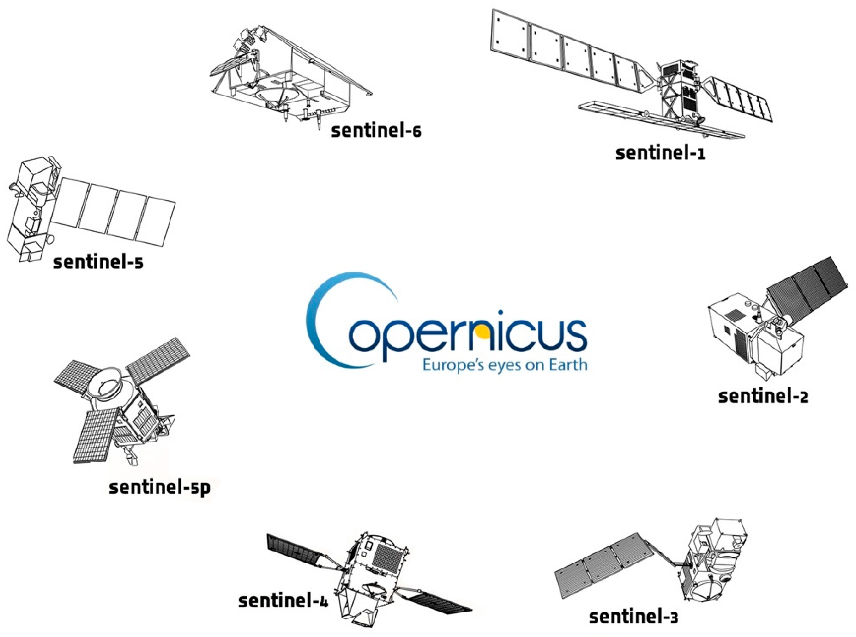
1.1. Sentinel-3
1.2. OLCI Products Are Available on Three Main Levels
1.3. The Case-2 Regional CoastColour Processor
2. Materials and Methods
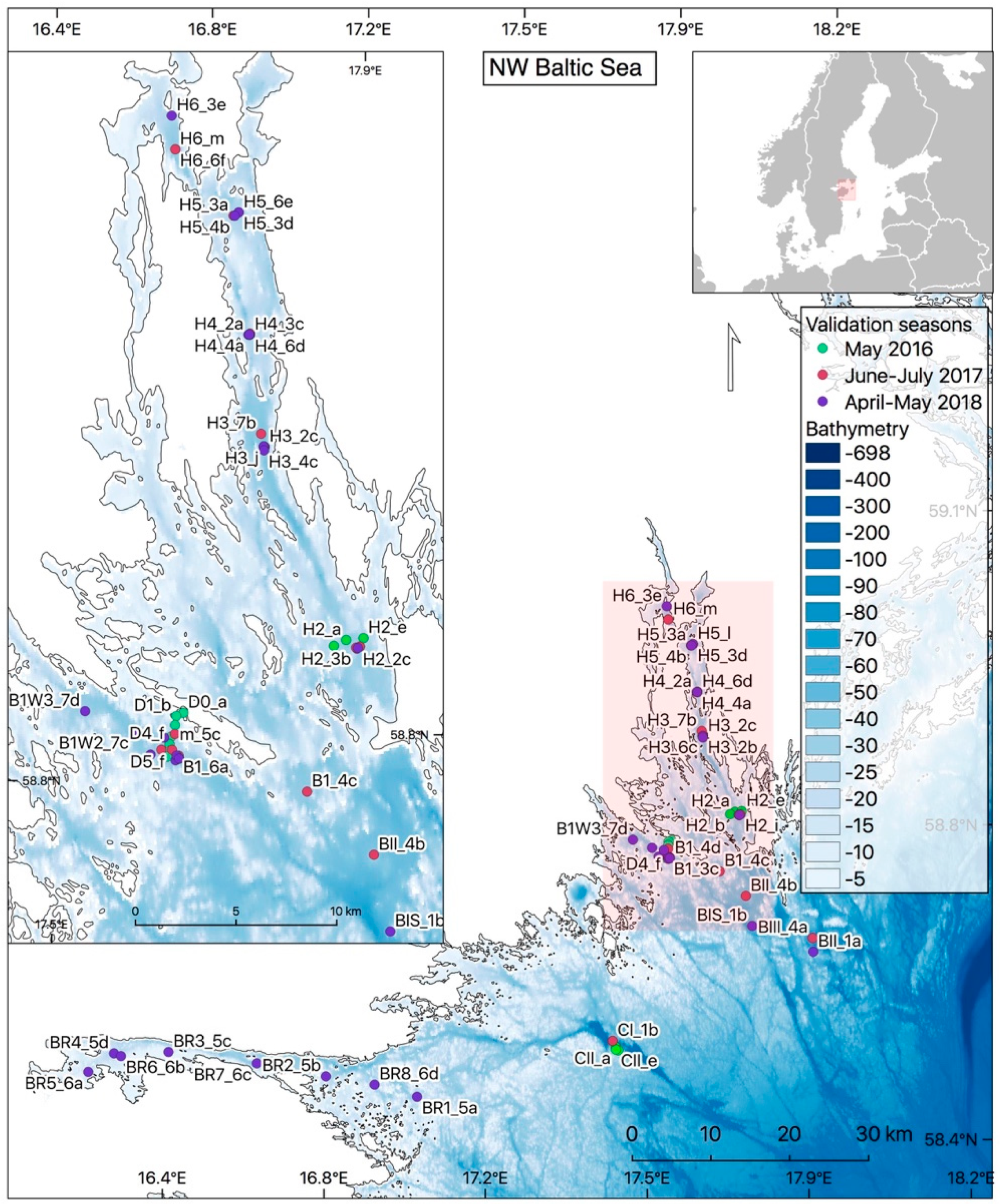
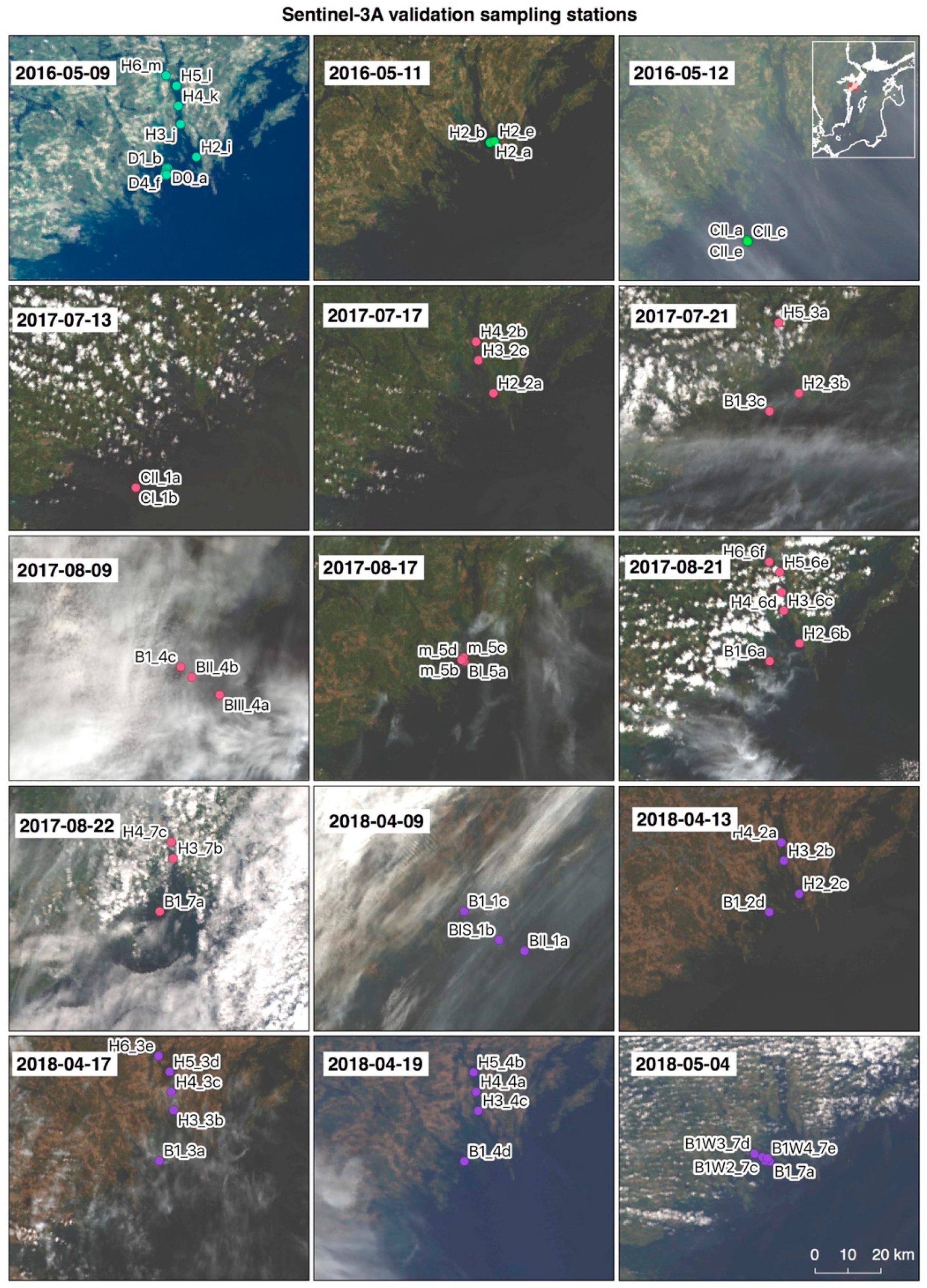
2.1. Area of Investigation
2.2. In Situ Sampling
2.3. Optical In-Situ Data
2.4. Satellite Data Processing
2.5. Turbidity Algorithm Development
2.6. Testing of Various Secchi Depth Algorithms
2.7. Statistical Evaluation of Match-up Data
3. Results
3.1. Remote Sensing Reflectance C2RCC-SNAP
3.2. Water Samples
3.3. Satellite-Derived Water Products in Relation to in Situ Water Samples
4. Discussion
4.1. Remote Sensing Reflectance
4.2. Level-2 Water Quality Products C2RCC-SNAP
5. Conclusions
Author Contributions
Funding
Acknowledgments
Conflicts of Interest
References
- Acker, J. How Two Sides of the Atlantic Contributed to Understanding of the Global Oceans: Charles Yentsch and Andre Morel. Limnol. Oceanogr. Bull. 2013, 22, 2–6. [Google Scholar] [CrossRef]
- Longhurst, A.; Sathyendranath, S.; Platt, T.; Caverhill, C. An estimate of global primary production in the ocean from satellite radiometer data. J. Plankton Res. 1995, 17, 1245–1271. [Google Scholar] [CrossRef]
- Behrenfeld, M.J.; O’Malley, R.T.; Siegel, D.A.; McClain, C.R.; Sarmiento, J.L.; Feldman, G.C.; Milligan, A.J.; Falkowski, P.G.; Letelier, R.M.; Boss, E.S. Climate-driven trends in contemporary ocean productivity. Nature 2006, 444, 752–755. [Google Scholar] [CrossRef] [PubMed]
- Bonekamp, H.; Montagner, F.; Santacesaria, V.; Loddo, C.N.; Wannop, S. Core operational Sentinel-3 marine data product services as part of the Copernicus Space Component. Ocean Sci. 2016, 12, 787–795. [Google Scholar] [CrossRef]
- Donlon, C.; Berruti, B.; Buongiorno, A.; Ferreira, M.; Féménias, P.; Frerick, J.; Goryl, P.; Klein, U.; Laur, H.; Mavrocordatos, C.; et al. Remote Sensing of Environment the Global Monitoring for Environment and Security (GMES) Sentinel-3 mission. Remote Sens. Environ. 2014, 120, 37–57. [Google Scholar] [CrossRef]
- ESA Overview / Copernicus / Observing the Earth / Our Activities / ESA. Available online: http://www.esa.int/Our_Activities/Observing_the_Earth/Copernicus/Overview4 (accessed on 10 August 2019).
- ESA Sentinel Family. Available online: https://www.esa.int/spaceinimages/Images/2014/04/Sentinel_family (accessed on 10 August 2019).
- ESA Sentinel-3 - Missions - Sentinel Online. Available online: https://sentinel.esa.int/web/sentinel/missions/sentinel-3 (accessed on 10 August 2019).
- Doerffer, R.; Sorensen, K.; Aiken, J. MERIS potential for coastal zone applications. Int. J. Remote Sens. 1999, 20, 1809–1818. [Google Scholar] [CrossRef]
- Moore, G.F.; Aiken, J.; Lavender, S.J. The atmospheric correction of water colour and the quantitative retrieval of suspended particulate matter in Case II waters: Application to MERIS. Int. J. Remote Sens. 1999, 20, 1713–1733. [Google Scholar] [CrossRef]
- Doerffer, R. Protocols for the Validation of MERIS Water Products; European Space Agency Doc. No. PO-TN-MEL-GS-0043; GKSS: Geesthacht, Germany, 2002; pp. 1–42. [Google Scholar]
- Merheim-Kealy, P.; Huot, J.P.; Delwart, S. The MERIS ground segment. Int. J. Remote Sens. 1999, 20, 1703–1712. [Google Scholar] [CrossRef]
- ESA. EUMETSAT Sentinel-3 OLCI Marine User Handbook Doc. No. EUM/OPS-SEN3/MAN/17/907205. v.1H. 2018. Available online: https://www.eumetsat.int/website/wcm/idc/idcplg?IdcService=GET_FILE&dDocName=PDF_DMT_907205&RevisionSelectionMethod=LatestReleased&Rendition=Web (accessed on 18 August 2018).
- ESA User Guides - Sentinel-3 OLCI - Heritage - Sentinel Online. Available online: https://sentinel.esa.int/web/sentinel/user-guides/sentinel-3-olci/overview/heritage (accessed on 10 August 2019).
- ESA—Sentinel Online User Guides-Sentinel-3 OLCI-Level-1b-Sentinel Online. Available online: https://sentinel.esa.int/web/sentinel/user-guides/sentinel-3-olci/product-types/level-1b (accessed on 10 August 2019).
- ESA—Sentinel Online User Guides-Sentinel-3 OLCI-Level-2 Water-Sentinel Online. Available online: https://sentinel.esa.int/web/sentinel/user-guides/sentinel-3-olci/product-types/level-2-water (accessed on 10 August 2019).
- Hieronymi, M.; Müller, D.; Doerffer, R. The OLCI Neural Network Swarm (ONNS): A Bio-Geo-Optical Algorithm for Open Ocean and Coastal Waters. Front. Mar. Sci. 2017, 4, 140. [Google Scholar] [CrossRef]
- Brockmann, C.; Doerffer, R.; Peters, M.; Stelzer, K.; Embacher, S.; Ruescas, A. Evolution of the C2RCC neural network for Sentinel 2 and 3 for the retrieval of ocean colour products in normal and extreme optically complex waters. In Proceedings of the Living Planet Symposium 2016, Prague, Czech Republic, 9–13 May 2016; pp. 9–13. [Google Scholar]
- Doerffer, R.; Schiller, H. The MERIS Case 2 water algorithm. Int. J. Remote Sens. 2007, 28, 517–535. [Google Scholar] [CrossRef]
- Sequoia Scientific HydroLight-Sequoia Scientific. Available online: https://www.sequoiasci.com/product/hydrolight/ (accessed on 10 August 2019).
- Chami, M.; Santer, R.; Dilligeard, E. Radiative transfer model for the computation of radiance and polarization in an ocean–atmosphere system: Polarization properties of suspended matter for remote sensing. Appl. Opt. 2007, 40, 2398. [Google Scholar] [CrossRef] [PubMed]
- Lenoble, J.; Herman, M.; Deuzé, J.L.; Lafrance, B.; Santer, R.; Tanré, D. A successive order of scattering code for solving the vector equation of transfer in the earth’s atmosphere with aerosols. J. Quant. Spectrosc. Radiat. Transf. 2007, 107, 479–507. [Google Scholar] [CrossRef]
- Kratzer, S.; Moore, G. Inherent Optical Properties of the Baltic Sea in Comparison to Other Seas and Oceans. Remote Sens. 2018, 10, 418. [Google Scholar] [CrossRef]
- Alikas, K.; Kratzer, S. Improved retrieval of Secchi depth for optically-complex waters using remote sensing data. Ecol. Indic. 2017, 77, 218–227. [Google Scholar] [CrossRef]
- Boesch, D.F.; Hecky, R.; O’Melia, C.; Schindler, D.; Seitzinger, S. Eutrophication of Swedish Seas; Swedish Environmental Protection Agency Naturvårdsverket: Stockholm, Sweden, 2006; ISBN 9162055097.
- Nyberg, S.; Larsson, U.; Walve, J. Himmerfjärden Eutrophication Study. Available online: http://www2.ecology.su.se/dbhfj/index.htm (accessed on 11 April 2019).
- EMODnet Shom (Service Hydrographique et Océanographique de la Marine) (2018). EMODnet Digital Bathymetry (DTM 2018). Available online: http://portal.emodnet-bathymetry.eu/ (accessed on 10 August 2018).
- HELCOM Subbasins 2018 Helcom Metadata Catalogue-Helcom. Available online: http://metadata.helcom.fi/geonetwork/srv/eng/catalog.search#/metadata/d4b6296c-fd19-462c-94d2-4c81b9313d77 (accessed on 10 August 2019).
- EEA Europe Coastline Shapefile. Available online: https://www.eea.europa.eu/ds_resolveuid/06227e40310045408ac8be0d469e1189 (accessed on 11 April 2019).
- Natural Earth Admin 0–Boundary Lines|Natural Earth. Available online: https://www.naturalearthdata.com/downloads/110m-cultural-vectors/110m-admin-0-boundary-lines/ (accessed on 10 August 2019).
- Vinterhav, C. Remote Sensing of Baltic Coastal Waters Using MERIS—A Comparison of Three Case-2 Water Processors. Master’s Thesis, Stockholm University, Stockholm, Sweden, 2008. [Google Scholar]
- Kyryliuk, D. Total Suspended Matter Derived from MERIS Data as an Indicator of Coastal Processes in the Baltic Sea. Master’s Thesis, Stockholm University, Stockholm, Sweden, 2014. [Google Scholar]
- ESA-ESOV ESOV. Available online: https://eop-cfi.esa.int/index.php/applications/esov (accessed on 10 August 2019).
- Kratzer, S.; Brockmann, C.; Moore, G. Using MERIS full resolution data to monitor coastal waters—A case study from Himmerfjarden, a fjord-like bay in the northwestern Baltic Sea. Remote Sens. Environ. 2008, 112, 2284–2300. [Google Scholar] [CrossRef]
- Kratzer, S.; Vinterhav, C. Improvement of MERIS level 2 products in baltic sea coastal areas by applying the improved Contrast between Ocean and Land Processor (ICOL)—Data analysis and validation. Oceanologia 2010, 52, 211–236. [Google Scholar] [CrossRef]
- Beltrán-Abaunza, J.M.; Kratzer, S.; Brockmann, C. Evaluation of MERIS products from Baltic Sea coastal waters rich in CDOM. Ocean Sci. 2014, 10, 377–396. [Google Scholar] [CrossRef]
- Zibordi, G.; Ruddick, K.; Ansko, I.; Moore, G.; Kratzer, S.; Icely, J.; Reinart, A. In situ determination of the remote sensing reflectance: An inter-comparison. Ocean Sci. 2012, 8, 567–586. [Google Scholar] [CrossRef]
- Strickland, J.D.H.; Parsons, T.R. A Practical Handbook of Seawater Analysis. A Pract. Handb. Seawater Anal. 1972, 167, 185. [Google Scholar] [CrossRef]
- Parsons, T.R.; Maita, Y.; Lalli, C.M. A Manual of Chemical and Biological Methods for Seawater Analysis. Geol. Mag. 1985, 122, 570. [Google Scholar] [CrossRef]
- Jeffrey, S.W.; Welschmeyer, N.A. Appendix F: Spectrophotometric and fluorometric equations in common use in oceanography. In Phytoplankton Pigments in Oceanography: Guidelines to Modern Methods; UNESCO Publishing: Paris, France, 1997; pp. 597–615. [Google Scholar]
- Kratzer, S.; Tett, P. Using bio-optics to investigate the extent of coastal waters: A Swedish case study. Hydrobiologia 2009, 629, 169–186. [Google Scholar] [CrossRef]
- Kirk, J.T.O.; John, T.O. Kirk: Light and photosynthesis in aquatic ecosystems. Int. Rev. Der Gesamten Hydrobiol. Und Hydrogr. 1985, 70, 897–898. [Google Scholar] [CrossRef]
- Kari, E.; Kratzer, S.; Beltrán-Abaunza, J.M.; Harvey, E.T.; Vaičiūtė, D. Retrieval of suspended particulate matter from turbidity–model development, validation, and application to MERIS data over the Baltic Sea. Int. J. Remote Sens. 2017, 38, 1983–2003. [Google Scholar] [CrossRef]
- EUMETSAT Copernicus Online Data Access (CODA) REProcessed. Available online: https://codarep.eumetsat.int (accessed on 10 August 2019).
- EUMETSAT Copernicus Online Data Access (CODA). Available online: https://coda.eumetsat.int (accessed on 10 August 2018).
- ESA. EUMETSAT S3 Product Notice–OLCI. Available online: https://www.eumetsat.int/website/wcm/idc/idcplg?IdcService=GET_FILE&dDocName=PDF_S3A_PN_OLCI_L1B_OCT&RevisionSelectionMethod=LatestReleased&Rendition=Web (accessed on 10 August 2019).
- ESA User Guides-Sentinel-3 OLCI-Naming Convention-Sentinel Online. Available online: https://sentinel.esa.int/web/sentinel/user-guides/sentinel-3-olci/naming-convention (accessed on 10 August 2019).
- ESA Science Toolbox Exploitation Platform (SNAP). Available online: http://step.esa.int/main/download/ (accessed on 10 August 2019).
- Philipson, P.; (Brockmann Geomatic Sweden AB). Personal communication, 2018.
- Cristina, S.; Goela, P.; Icely, J. Assessment of water-leaving reflectances of oceanic and coastal waters using MERIS satellite products off the southwest coast of Portugal. J. Coast. Res. 2009, 2, 1479–1483. [Google Scholar]
- Lee, Z.P.; Du, K.P.; Arnone, R. A model for the diffuse attenuation coefficient of downwelling irradiance. J. Geophys. Res. C Ocean. 2005, 110, 1–10. [Google Scholar] [CrossRef]
- Harvey, E.T.; Walve, J.; Andersson, A.; Karlson, B.; Kratzer, S. The Effect of Optical Properties on Secchi Depth and Implications for Eutrophication Management. Front. Mar. Sci. 2019, 5, 1–19. [Google Scholar] [CrossRef]
- Toming, K.; Kutser, T.; Laas, A.; Sepp, M.; Paavel, B.; Nõges, T. First experiences in mapping lakewater quality parameters with sentinel-2 MSI imagery. Remote Sens. 2016, 8, 640. [Google Scholar] [CrossRef]
- Morel, A.; Prieur, L. Analysis of variations in ocean color. Limnol. Oceanogr. 1977, 22, 709–722. [Google Scholar] [CrossRef]
- Kutser, T.; Paavel, B.; Metsamaa, L.; Vahtmäe, E. Mapping coloured dissolved organic matter concentration in coastal waters. Int. J. Remote Sens. 2009, 30, 5843–5849. [Google Scholar] [CrossRef]
- Harvey, T.; Kratzer, S.; Andersson, A. Relationships between colored dissolved organic matter and dissolved organic carbon in different coastal gradients of the Baltic Sea. Ambio 2015, 44, 392–401. [Google Scholar] [CrossRef]
- Siegel, H.; Gerth, M.; Ohde, T.; Heene, T. Ocean colour remote sensing relevant water constituents and optical properties of the Baltic Sea. Int. J. Remote Sens. 2005, 26, 315–330. [Google Scholar] [CrossRef]
- Fan, Y.; Li, W.; Gatebe, C.K.; Jamet, C.; Zibordi, G.; Schroeder, T.; Stamnes, K. Atmospheric correction over coastal waters using multilayer neural networks. Remote Sens. Environ. 2017, 199, 218–240. [Google Scholar] [CrossRef]
- Attila, J.; Koponen, S.; Kallio, K.; Lindfors, A.; Kaitala, S.; Ylostalo, P. MERIS Case II water processor comparison on coastal sites of the northern Baltic Sea. Remote Sens. Environ. 2013, 128, 138–149. [Google Scholar] [CrossRef]
- Ohde, T.; Siegel, H.; Gerth, M. Validation of MERIS Level-2 products in the Baltic Sea, the Namibian coastal area and the Atlantic Ocean. Int. J. Remote Sens. 2007, 28, 609–624. [Google Scholar] [CrossRef]
- Vaičiūtė, D.; Bresciani, M.; Bučas, M. Validation of MERIS bio-optical products with in situ data in the turbid Lithuanian Baltic Sea coastal waters. J. Appl. Remote Sens. 2012, 6, 063568. [Google Scholar] [CrossRef]
- Santer, R.; Zagolski, F. ICOL—Improve Contrast between Ocean & Land, ATBD (Algorithm Theoretical Basis Document)—MERIS Level-1C; Version: 1.1. Available online: http://www.brockmann-consult.de/beam-wiki/download/attachments/13828113/ICOL_ATBD_1.1.pdf (accessed on 18 August 2019).
- Sterckx, S.; Knaeps, S.; Kratzer, S.; Ruddick, K. SIMilarity Environment Correction (SIMEC) applied to MERIS data over inland and coastal waters. Remote Sens. Environ. 2015, 157, 96–110. [Google Scholar] [CrossRef]
- Schroeder, T.; Behnert, I.; Schaale, M.; Fischer, J.; Doerffer, R. Atmospheric correction algorithm for MERIS above case-2 waters. Int. J. Remote Sens. 2007, 28, 1469–1486. [Google Scholar] [CrossRef]
- Schroeder, T.; Schaale, M.; Fischer, J. Retrieval of atmospheric and oceanic properties from MERIS measurements: A new Case-2 water processor for BEAM. Int. J. Remote Sens. 2007, 28, 5627–5632. [Google Scholar] [CrossRef]
- Kratzer, S.; Kowalczuk, P.; Sagan, S. Bio-optical water quality assessment. Chapter 15. In Biological Oceanography of the Baltic Sea; Snoeijs-Leijonmalm, P., Schubert, H., Radziejewska, T., Eds.; Springer International Publishing: Cham, Switzerland, 2017; pp. 527–545. ISBN 978-94-007-0668-2. [Google Scholar]
- Sagan, S. The Inherent Water Optical Properties of Baltic Waters. Diss. Monogr. Inst. Oceanol. PAS 2008, 21, 244. (In Polish) [Google Scholar]
- Doerffer, R.; Schiller, H. The MERIS neural network algorithm. In Remote Sensing of Inherent Optical Properties: Fundamentals, Tests of Algorithms and Applications; Lee, Z.P., Ed.; International Ocean Colour Coordinating Group: Halifax, NS, Canada, 2007. [Google Scholar]
- Heim, B.; Overduin, P.; Schirrmeister, L.; Doerffer, R. OCOC-from Ocean Colour to Organic Carbon. Available online: https://epic.awi.de/id/eprint/19457/1/Hei2008g.pdf (accessed on 18 August 2019).
- Plowey, M. A Multi-Scale Approach to Monitoring the Optically Complex Coastal Waters of the Baltic Sea—A Comparison of Satellite, Mooring, and Ship-Based Monitoring of Ocean Colour. Master’s Thesis, Stockholm University, Stockholm, Sweden, 2019. [Google Scholar]
- Blix, K.; Pálffy, K.; Tóth, V.R.; Eltoft, T. Remote sensing of water quality parameters over Lake Balaton by using Sentinel-3 OLCI. Water (Switz.) 2018, 10, 1428. [Google Scholar] [CrossRef]
- Mollaee, S. Estimation of Phytoplankton Chlorophyll-a Concentration in the Western Basin of Lake Erie Using Sentinel-2 and Sentinel-3 Data. Master’s Thesis, University of Waterloo, Waterloo, ON, Canada, 2018. [Google Scholar]
- Kratzer, S.; Håkansson, B.; Sahlin, C. Assessing Secchi and photic zone depth in the Baltic Sea from satellite data. J. Hum. Environ. 2003, 32, 577–585. [Google Scholar] [CrossRef]
- Hooker, S.B.; Mcclain, C.R. The calibration and validation of SeaWiFS data. Prog. Oceanogr. 2000, 45, 427–465. [Google Scholar] [CrossRef]
- Doron, M.; Babin, M.; Hembise, O.; Mangin, A.; Garnesson, P. Ocean transparency from space: Validation of algorithms estimating Secchi depth using MERIS, MODIS and SeaWiFS data. Remote Sens. Environ. 2011, 115, 2986–3001. [Google Scholar] [CrossRef]
- Kratzer, S.; Therese Harvey, E.; Philipson, P. The use of ocean color remote sensing in integrated coastal zone management—A case study from Himmerfjärden, Sweden. Mar. Policy 2014, 43, 29–39. [Google Scholar] [CrossRef]
- Jerlov, N.G. Marine Optics; Elsevier O.: Amsterdam, The Netherlands, 1976; Volume 14, ISBN 0075-7535. [Google Scholar]
- Fleming-Lehtinen, V. Secchi Depth in the Baltic Sea—An Indicator of Eutrophication. Ph.D. Thesis, Faculty of Biological and Environmental Sciences of the University of Helsinki, 2016. [Google Scholar]
- Fleming-Lehtinen, V.; Laamanen, M. Long-term changes in Secchi depth and the role of phytoplankton in explaining light attenuation in the Baltic Sea. Estuar. Coast. Shelf Sci. 2012, 102, 1–10. [Google Scholar] [CrossRef]
- Stock, A. Satellite mapping of Baltic Sea Secchi depth with multiple regression models. Int. J. Appl. Earth Obs. Geoinf. 2015, 40, 55–64. [Google Scholar] [CrossRef]
- Nechad, B.; Ruddick, K.G.; Neukermans, G. Calibration and validation of a generic multisensor algorithm for mapping turbidity in coastal waters. SPIE Eur. Remote Sens. 2009, 7473, 74730H. [Google Scholar] [CrossRef]
- Dogliotti, A.I.; Ruddick, K.G.; Nechad, B.; Doxaran, D.; Knaeps, E. A single algorithm to retrieve turbidity from remotely-sensed data in all coastal and estuarine waters. Remote Sens. Environ. 2015, 156, 157–168. [Google Scholar] [CrossRef]
- Marine Strategy Framework Directive Annex III Directive 2008/56/EC of the European Parliament and of the Council. Off. J. Eur. Union 2008, 164, 19–40.
- Harvey, T. Bio-Optics, Satellite Remote Sensing and Baltic Sea Ecosystems. Ph.D. Thesis, Faculty of Science, Department of Ecology, Environment and Plant Sciences, Stockholm University, Stockholm, Sweden, 2015. [Google Scholar]
- Beltrán-Abaunza, J.M. Remote Sensing in Optically Complex Waters: Water Quality Assessment Using MERIS Data. Ph.D. Thesis, Faculty of Science, Department of Ecology, Environment and Plant Sciences, Stockholm University, Stockholm, Sweden, 2015. [Google Scholar]


| Band i.d. | Center Wavelength (nm) | Bandwidth (nm) |
|---|---|---|
| Oa1 | 400 | 15 |
| Oa2 | 412.5 | 10 |
| Oa3 | 442.5 | 10 |
| Oa4 | 490 | 10 |
| Oa5 | 510 | 10 |
| Oa6 | 560 | 10 |
| Oa7 | 620 | 10 |
| Oa8 | 665 | 10 |
| Oa9 | 673.75 | 7.5 |
| Oa10 | 681.25 | 7.5 |
| Oa11 | 708.75 | 10 |
| Oa12 | 753.75 | 7.5 |
| Oa13 | 761.25 | 2.5 |
| Oa14 | 764.375 | 3.75 |
| Oa15 | 767.5 | 2.5 |
| Oa16 | 778.75 | 15 |
| Oa17 | 865 | 20 |
| Oa18 | 885 | 10 |
| Oa19 | 900 | 10 |
| Oa20 | 940 | 20 |
| Oa21 | 1020 | 40 |
| Time [UTC + 0] | Sentinel-3 Matchup Window | |||||||
|---|---|---|---|---|---|---|---|---|
| Cast ID | Date | In situ | Overpass Start | Cloudy | <30 min | ≤1 h | ≤2 h | >2 h |
| D0_a | 9 May 2016 | 09:39:00 | 08:58:42 | * | ||||
| D1_b | 10:04:00 | 08:58:42 | * | |||||
| D2_c | 10:18:00 | 08:58:42 | * | |||||
| D3_d | 10:32:00 | 08:58:42 | * | |||||
| D4_f | 10:45:00 | 08:58:42 | * | |||||
| D5_f | 10:57:00 | 08:58:42 | * | |||||
| D6_g | 11:09:00 | 08:58:42 | * | |||||
| B1_h | 05:20:00 | 08:58:42 | * | |||||
| H2_i | 06:42:00 | 08:58:42 | * | |||||
| H3_j | 09:50:00 | 08:58:42 | * | |||||
| H4_k | 07:35:00 | 08:58:42 | * | |||||
| H5_l | 08:10:00 | 08:58:42 | * | |||||
| H6_m | 08:30:00 | 08:58:42 | * | |||||
| H2_a | 11 May 2016 | 09:09:00 | 09:47:19 | ** | * | |||
| H2_b | 09:39:00 | 09:47:19 | ** | * | ||||
| H2_e | 10:17:00 | 09:47:19 | ** | * | ||||
| CII_a | 11 May 2016 | 08:58:00 | 09:21:07 | * | ||||
| CII_c | 09:57:00 | 09:21:07 | * | |||||
| CII_e | 11:20:00 | 09:21:07 | * | |||||
| CII_1a | 13 July 2017 | 08:45:00 | 09:51:11 | * | ||||
| CI_1b | x | 09:51:11 | ||||||
| CI_1c | x | 09:51:11 | ||||||
| H2_2a | 17 July 2017 | 08:25:00 | 09:47:27 | * | ||||
| H4_2b | 10:15:00 | 09:47:27 | * | |||||
| H3_2c | 11:10:00 | 09:47:27 | * | |||||
| H5_3a | 21 July 2017 | 08:30:00 | 09:43:42 | ** | * | |||
| H2_3b | 10:12:00 | 09:43:42 | * | |||||
| B1_3c | 11:15:00 | 09:43:42 | ** | * | ||||
| BIII_4a | 9 Aug. 2017 | 08:25:00 | 09:51:10 | ** | * | |||
| BII_4b | 10:45:00 | 09:51:10 | ** | * | ||||
| B1_4c | 12:45:00 | 09:51:10 | ** | * | ||||
| BI_5a | 17 Aug. 2017 | 07:15:00 | 09:43:40 | * | ||||
| m_5b | 07:40:00 | 09:43:40 | * | |||||
| m_5c | 08:05:00 | 09:43:40 | * | |||||
| m_5d | 08:35:00 | 09:43:40 | * | |||||
| B1_6a | 21 Aug. 2017 | 05:45:00 | 09:39:55 | * | ||||
| H2_6b | 07:10:00 | 09:39:55 | * | |||||
| H3_6c | 09:08:00 | 09:39:55 | * | |||||
| H4_6d | 08:15:00 | 09:39:55 | * | |||||
| H5_6e | 11:36:00 | 09:39:55 | * | |||||
| H6_6f | x | 09:39:55 | ||||||
| B1_7a | 22 Aug. 2017 | 07:10:00 | 09:13:42 | * | ||||
| H3_7b | 08:15:00 | 09:13:42 | ** | * | ||||
| H4_7c | 08:45:00 | 09:13:42 | ** | * | ||||
| BII_1a | 9 April 2018 | 08:30:00 | 09:51:11 | ** | * | |||
| BIS_1b | 09:50:00 | 09:51:11 | ** | * | ||||
| B1_1c | 11:10:00 | 09:51:11 | ** | * | ||||
| H4_2a | 13 April 2018 | 08:03:00 | 09:47:26 | * | ||||
| H3_2b | 09:17:00 | 09:47:26 | * | |||||
| H2_2c | 10:57:00 | 09:47:26 | * | |||||
| B1_2d | 11:55:00 | 09:47:26 | * | |||||
| B1_3a | 17 April 2018 | 06:20:00 | 09:43:42 | ** | * | |||
| H3_3b | 08:55:00 | 09:43:42 | * | |||||
| H4_3c | 08:05:00 | 09:43:42 | * | |||||
| H5_3d | 10:52:00 | 09:43:42 | * | |||||
| H6_3e | 10:20:00 | 09:43:42 | * | |||||
| H4_4a | 19 April 2018 | 08:10:00 | 08:51:20 | * | ||||
| H5_4b | 09:22:00 | 08:51:20 | * | |||||
| H3_4c | 11:35:00 | 08:51:20 | * | |||||
| B1_4d | 13:30:00 | 08:51:20 | * | |||||
| B1_7a | 4 May 2018 | 08:45:00 | 09:02:33 | * | ||||
| B1W_7b | 09:01:00 | 09:02:33 | * | |||||
| B1W2_7c | 09:10:00 | 09:02:33 | * | |||||
| B1W3_7d | 09:19:00 | 09:02:33 | * | |||||
| B1W4_7e | 09:34:00 | 09:02:33 | * | |||||
| List of Level-1 Full Resolution OLCI Products | Products Availability |
|---|---|
| S3A_OL_1_EFR____20160509T085842_20160509T090042_20170929T065132_0119_004_050______MR1_R_NT_002.SEN3 | CODArep (https://codarep.eumetsat.int) |
| S3A_OL_1_EFR____20160511T094719_20160511T094919_20170929T091509_0119_004_079______MR1_R_NT_002.SEN3 | |
| S3A_OL_1_EFR____20160512T092107_20160512T092307_20170929T102634_0119_004_093______MR1_R_NT_002.SEN3 | |
| S3A_OL_1_EFR____20170713T095111_20170713T095311_20171021T102121_0119_020_022______MR1_R_NT_002.SEN3 | |
| S3A_OL_1_EFR____20170717T094727_20170717T094927_20171021T171336_0119_020_079______MR1_R_NT_002.SEN3 | |
| S3A_OL_1_EFR____20170721T094342_20170721T094542_20171022T000942_0119_020_136______MR1_R_NT_002.SEN3 | |
| S3A_OL_1_EFR____20170809T095110_20170809T095310_20171216T030232_0119_021_022______MR1_R_NT_002.SEN3 | |
| S3A_OL_1_EFR____20170817T094340_20170817T094540_20171216T125353_0119_021_136______MR1_R_NT_002.SEN3 | |
| S3A_OL_1_EFR____20170821T093955_20170821T094155_20171216T174456_0119_021_193______MR1_R_NT_002.SEN3 | |
| S3A_OL_1_EFR____20170822T091342_20170822T091542_20171216T185333_0119_021_207______MR1_R_NT_002.SEN3 | |
| S3A_OL_1_EFR____20180409T095111_20180409T095411_20180410T153428_0179_030_022_1980_MAR_O_NT_002.SEN3 | CODA (https://coda.eumetsat.int) |
| S3A_OL_1_EFR____20180413T094726_20180413T095026_20180414T160621_0179_030_079_1980_MAR_O_NT_002.SEN3 | |
| S3A_OL_1_EFR____20180417T094342_20180417T094642_20180418T152141_0180_030_136_1980_MAR_O_NT_002.SEN3 | |
| S3A_OL_1_EFR____20180419T085120_20180419T085420_20180420T141404_0179_030_164_1980_MAR_O_NT_002.SEN3 | |
| S3A_OL_1_EFR____20180504T090233_20180504T090533_20180505T140824_0179_030_378_1980_MAR_O_NT_002.SEN3 |
| C2RCC OLCI Processing Parameters. | |||
|---|---|---|---|
| Date | May 2016 | July–August 2017 | April–May 2018 |
| Valid-pixel expression | default | default | default |
| Salinity | 7 | 7 | 7 |
| Temperature | 5 | 15 | 5 |
| Ozone | 330 * | 330 * | 330 * |
| Air Pressure | 1000 * | 1000 * | 1000 * |
| TSM factor bpart | 0.986 ** | 0.986 ** | 0.986 ** |
| TSM factor bwit | 1.72 | 1.72 | 1.72 |
| CHL exponent | 1.04 | 1.04 | 1.04 |
| CHL factor | 21 | 21 | 21 |
| Threshold rtosa OOS | 0.05 | 0.05 | 0.05 |
| Threshold AC reflectances OOS | 0.1 | 0.1 | 0.1 |
| Threshold for cloud flag on transmittance down @865 | 0.955 | 0.955 | 0.955 |
| Atmospheric aux data path | default | default | default |
| Alternative NN Path | default | default | default |
| Output AC reflectances as Rrs instead of rhow | On | On | On |
| Derive water reflectance from path radiance and transmittance | Off | Off | Off |
| Use ECMWF aux data of source product | On | On | On |
| Output TOA reflectances | On | On | On |
| Output gas corrected TOSA reflectances | Off | Off | Off |
| Output gas corrected TOSA reflectances of auto NN | Off | Off | Off |
| Output path radiance reflectances | Off | Off | Off |
| Output downward transmittance | Off | Off | Off |
| Output upward transmittance | Off | Off | Off |
| Output atmospherically corrected angular dependent reflectances | On | On | On |
| Output normalized water-leaving reflectances | On | On | On |
| Output of out of scope values | Off | Off | Off |
| Output of irradiance attenuation coefficients | On | On | On |
| Output uncertainties | On | On | On |
| Output L2 Products Generated by C2RCC | ||
|---|---|---|
| Product Name | Description | Unit |
| Rtoa 400–1020 nm | Top-of-atmosphere reflectance | |
| Rrs 400–1020 nm | Atmospherically corrected angular dependent remote sensing reflectances | sr−1 |
| Rhow 400–1020 nm | Atmospherically corrected angular dependent water-leaving reflectances, Rhow = Rrs × π | |
| Diffuse attenuation coefficicent | ||
| kd489 | Irradiance attenuation coefficient at 489 nm | m−1 |
| kdmin | Mean irradiance attenuation coefficient at the three bands with minimum kd | m−1 |
| kd_z90max | Depth of the water column from which 90% of the water-leaving irradiance comes from (1/kdmin) | m |
| Inherent optical properties | ||
| iop_apig | Absorption coefficient of phytoplankton pigments at 443 nm | m−1 |
| iop_adet | Absorption coefficient of detritus at 443 nm | m−1 |
| iop_agelb | Absorption coefficient of Gelbstoff at 443 nm | m−1 |
| iop_bpart | Scattering coefficient of marine particles at 443 nm | m−1 |
| iop_bwit | Scattering coefficient of white particles at 443 nm | m−1 |
| iop_adg | Detritus + gelbstoff absorption at 443 nm (iop_adet + iop_agelb) | m−1 |
| iop_atot | phytoplankton + detritus + gelbstoff absorption at 443 nm (iop_apig + iop_adet + iop_agelb) | m−1 |
| iop_btot | total particle scattering at 443 nm (iop_bpart + iop_bwit) | m−1 |
| Concentrations (conc) | ||
| conc_tsm | Total suspended matter dry weight concentration (iop_bpart × 0.986 + iop_bwit × 1.72) | gm−3 |
| conc_chl | Chlorophyll concentration (pow (iop_apig, 1.04) × 21.0) | µgL−1 |
| User-defined | ||
| SD | Secchi depth = 2.39 × (kd489−0.86) [24] | m |
| Turb1 | Turbidity = 0.99 × iop_bpart + 0.24 | FNU |
| Turb2 | Turbidity = exp ((0.82 × ln (iop_bpart) + 0.14) | FNU |
© 2019 by the authors. Licensee MDPI, Basel, Switzerland. This article is an open access article distributed under the terms and conditions of the Creative Commons Attribution (CC BY) license (http://creativecommons.org/licenses/by/4.0/).
Share and Cite
Kyryliuk, D.; Kratzer, S. Evaluation of Sentinel-3A OLCI Products Derived Using the Case-2 Regional CoastColour Processor over the Baltic Sea. Sensors 2019, 19, 3609. https://doi.org/10.3390/s19163609
Kyryliuk D, Kratzer S. Evaluation of Sentinel-3A OLCI Products Derived Using the Case-2 Regional CoastColour Processor over the Baltic Sea. Sensors. 2019; 19(16):3609. https://doi.org/10.3390/s19163609
Chicago/Turabian StyleKyryliuk, Dmytro, and Susanne Kratzer. 2019. "Evaluation of Sentinel-3A OLCI Products Derived Using the Case-2 Regional CoastColour Processor over the Baltic Sea" Sensors 19, no. 16: 3609. https://doi.org/10.3390/s19163609
APA StyleKyryliuk, D., & Kratzer, S. (2019). Evaluation of Sentinel-3A OLCI Products Derived Using the Case-2 Regional CoastColour Processor over the Baltic Sea. Sensors, 19(16), 3609. https://doi.org/10.3390/s19163609