A Comparable Study of CNN-Based Single Image Super-Resolution for Space-Based Imaging Sensors


Abstract
1. Introduction
2. Methods and Network Structures
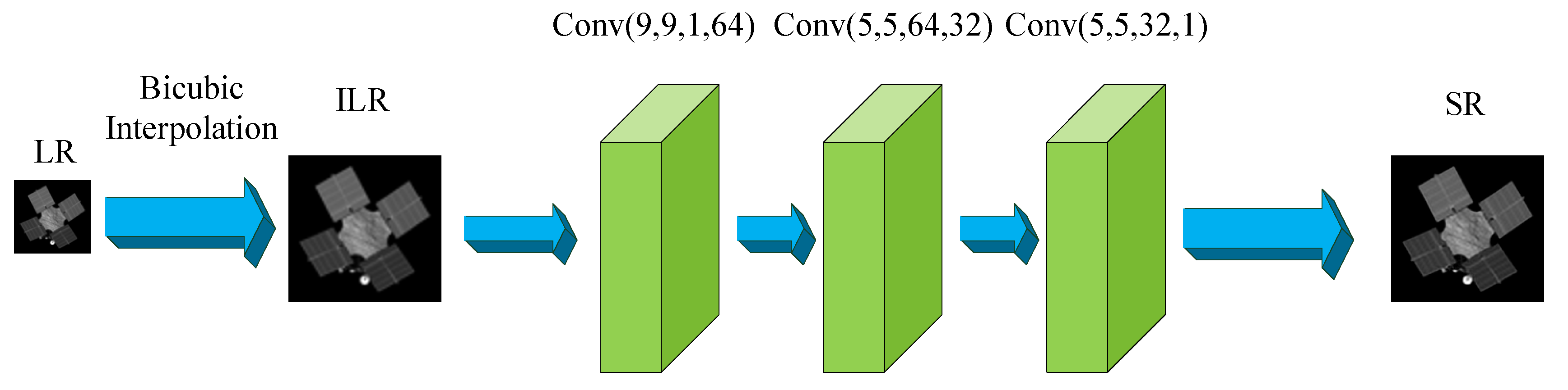
2.1. SRCNN
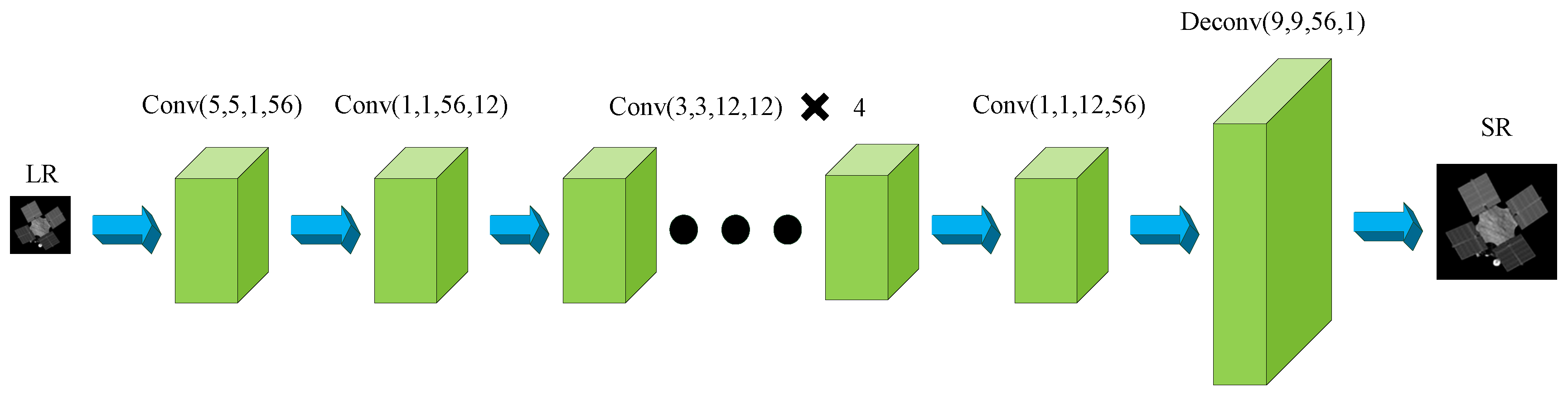
2.2. FSRCNN
2.3. VDSR
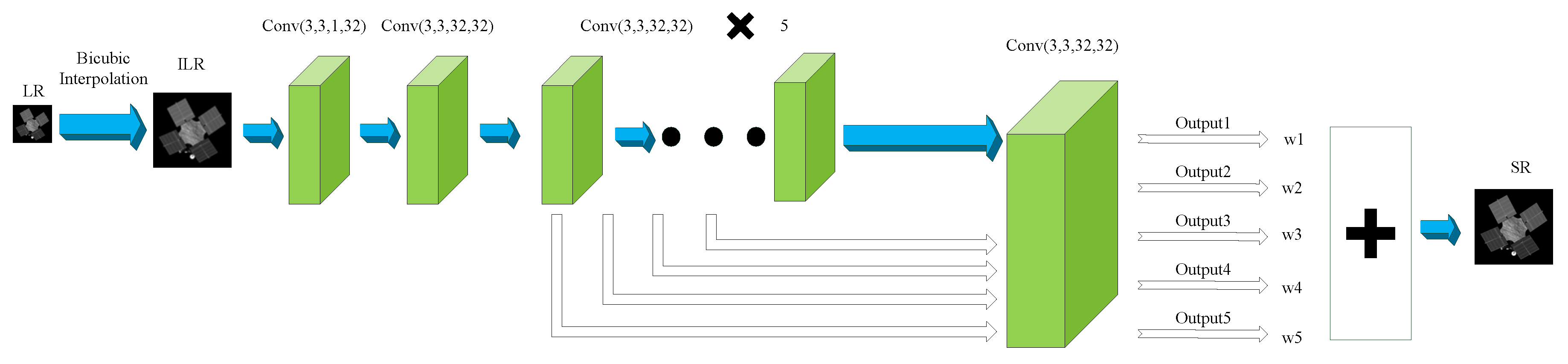
2.4. DRCN
3. Experiments and Analyses
3.1. Dataset
3.2. Index for Evaluation
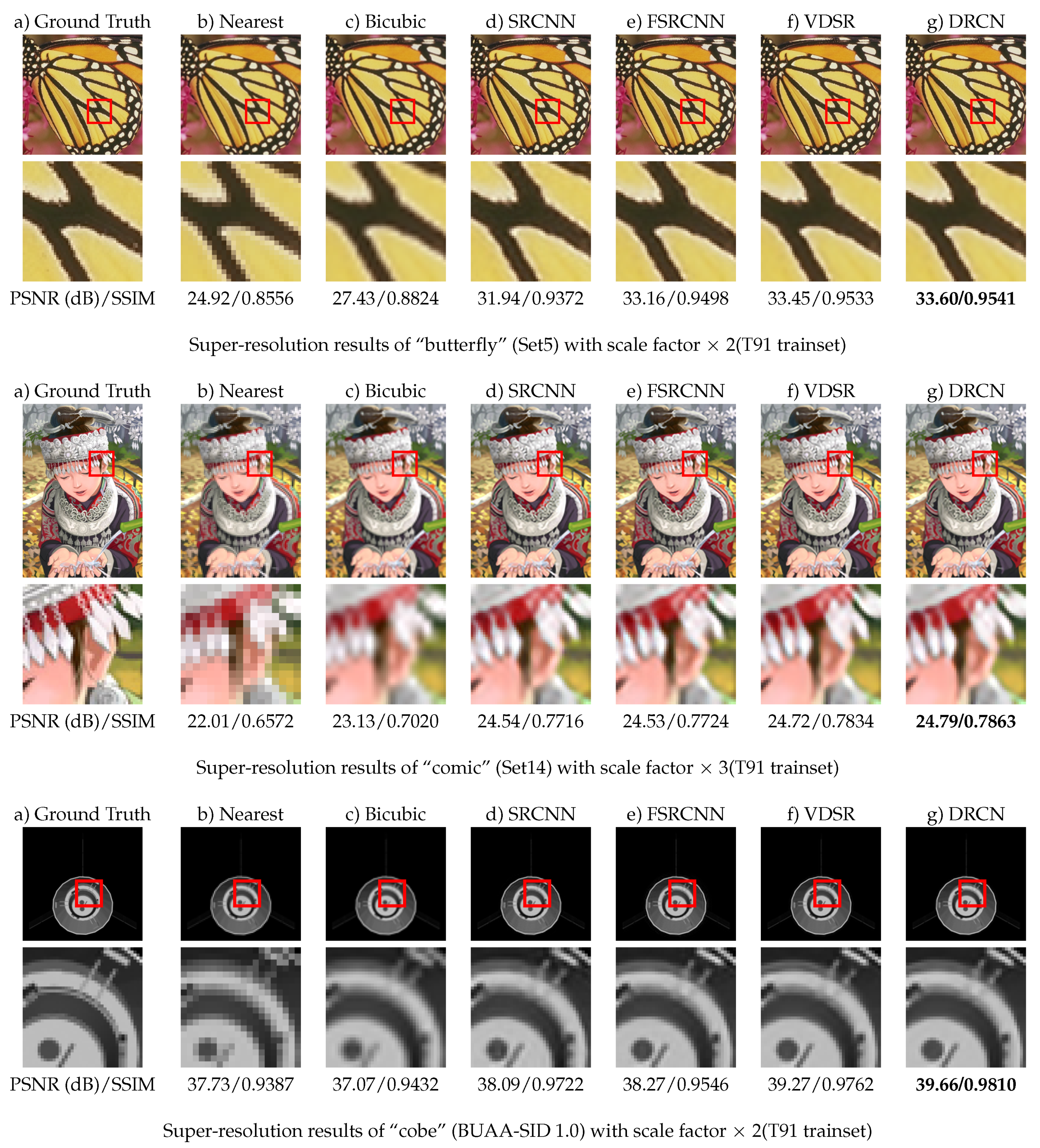
3.3. Training with Natural Images in Fixed Scale
3.4. Training with Natural Images in Multiple Scales
3.5. Training with Space Object Images
3.5.1. Comparison of Fixed Scale and Multiple Scale
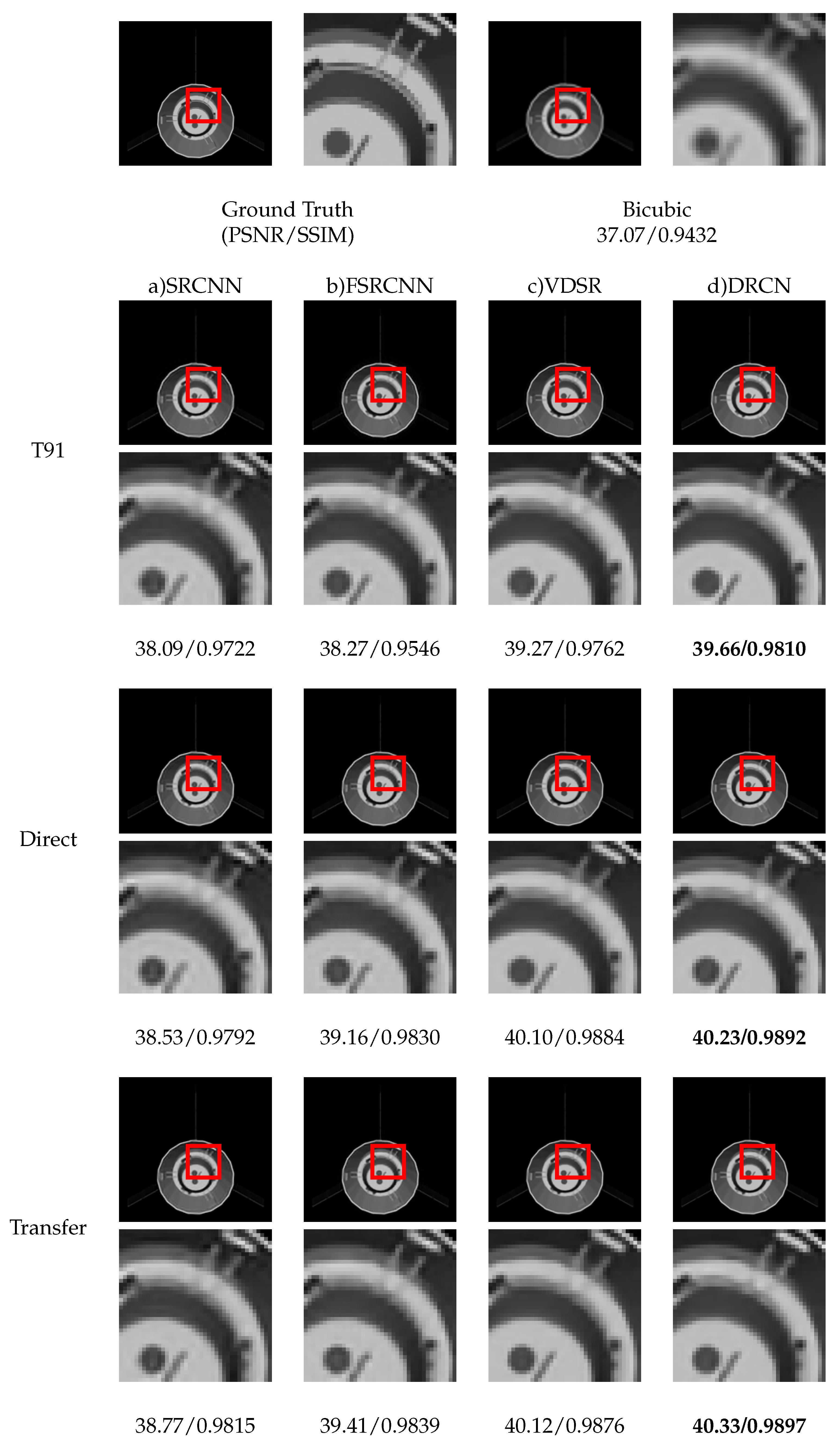
3.5.2. Comparison of Direct Training and Transfer Training
3.5.3. Computational Complexity
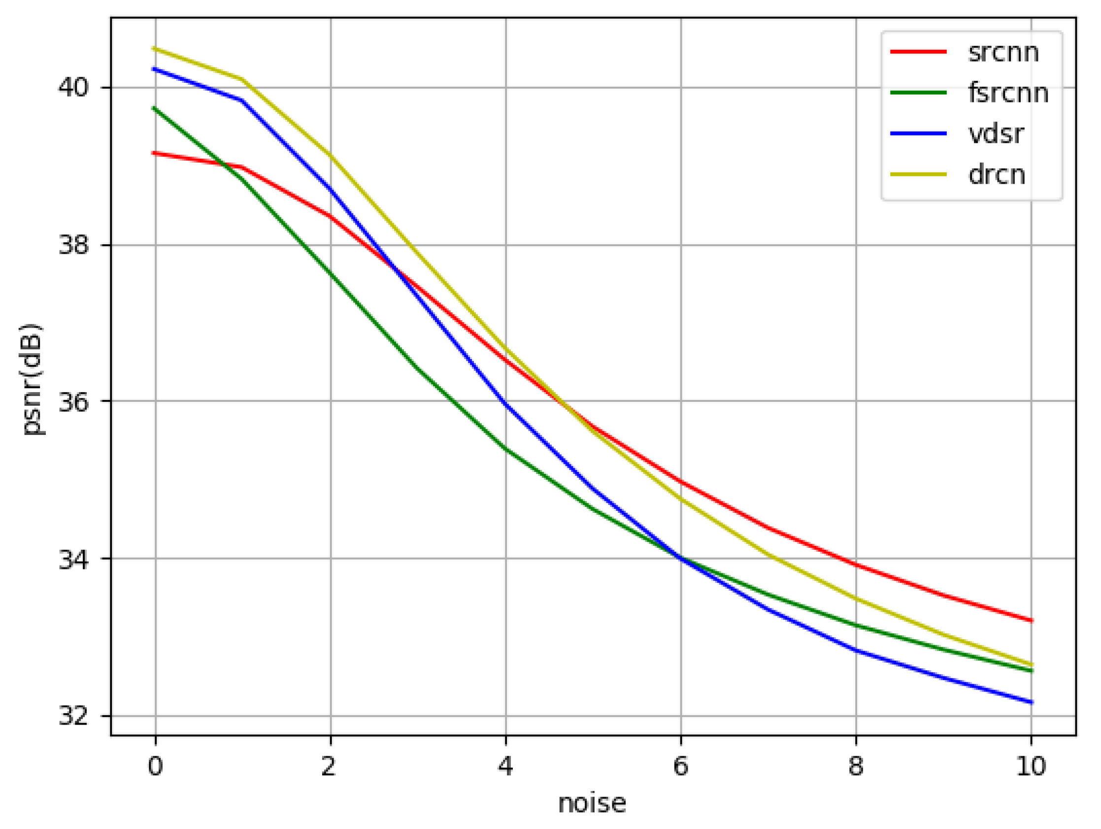
3.5.4. Noise Robustness
4. Discussion
5. Conclusions
Author Contributions
Funding
Conflicts of Interest
References
- Space based Space Surveillance (SBSS). 2016. Available online: https://www.globalsecurity.org/space/systems/sbss.htm (accessed on 24 January 2018).
- NEOSSat: Canada’s Sentinel in the Sky. 2015. Available online: http://www.asc-csa.gc.ca/eng/satellites/neossat (accessed on 24 January 2018).
- Kelsey, J.; Byrne, J.; Cosgrove, M.; Seereeram, S.; Mehra, R. Vision-based relative pose estimation for autonomous rendezvous and docking. In Proceedings of the IEEE Aerospace Conference, Big Sky, MT, USA, 4–11 March 2006; pp. 1–20. [Google Scholar] [CrossRef]
- Petit, A.; Marchand, E.; Kanani, K. Vision-based space autonomous rendezvous: A case study. In Proceedings of the IEEE/RSJ International Conference on Intelligent Robots and Systems, San Francisco, CA, USA, 25–30 September 2011; pp. 619–624. [Google Scholar]
- Liu, C.; Hu, W. Relative pose estimation for cylinder-shaped spacecrafts using single image. IEEE Trans. Aerosp. Electron. Syst. 2014, 50, 3036–3056. [Google Scholar] [CrossRef]
- Rogata, P.; Sotto, E.D.; Camara, F.; Caramagno, A.; Rebordao, J.M.; Correia, B.; Duarte, P.; Mancuso, S. Design and performance assessment of hazard avoidance techniques for vision-based landing. Acta Astronaut. 2007, 61, 63–77. [Google Scholar] [CrossRef]
- Segal, S.; Carmi, A.; Gurfil, P. Vision-based relative state estimation of non-cooperative spacecraft under modeling uncertainty. In Proceedings of the IEEE Aerospace Conference, Big Sky, MT, USA, 5–12 March 2011; pp. 1–8. [Google Scholar] [CrossRef]
- Zhang, H.; Jiang, Z.; Elgammal, A. Vision-Based Pose Estimation for Cooperative Space Objects. Acta Astronaut. 2013, 91, 115–122. [Google Scholar] [CrossRef]
- Opromolla, R.; Fasano, G.; Rufino, G.; Grassi, M. Pose Estimation for Spacecraft Relative Navigation Using Model-Based Algorithms. IEEE Trans. Aerosp. Electron. Syst. 2017, 53, 431–447. [Google Scholar] [CrossRef]
- Zhang, X.; Jiang, Z.; Zhang, H.; Wei, Q. Vision-Based Pose Estimation for Textureless Space Objects by Contour Points Matching. IEEE Trans. Aerosp. Electron. Syst. 2018, 54, 2342–2355. [Google Scholar] [CrossRef]
- Zhang, G.; Liu, H.; Wang, J.; Jiang, L. Vision-Based System for Satellite On-Orbit Self-Servicing. In Proceedings of the IEEE/ASME International Conference on Advanced Intelligent Mechatronics, Xi’an, China, 2–5 July 2008; pp. 296–301. [Google Scholar] [CrossRef]
- Flores-Abad, A.; Ma, O.; Pham, K.; Ulrich, S. A review of space robotics technologies for on-orbit servicing. Prog. Aerosp. Sci. 2014, 68, 1–26. [Google Scholar] [CrossRef]
- Benninghoff, H.; Boge, T.; Rems, F. Autonomous navigation for on-orbit servicing. KI-Künstl. Intell. 2014, 28, 77–83. [Google Scholar] [CrossRef]
- van Hecke, K.; de Croon, G.C.; Hennes, D.; Setterfield, T.P.; Saenz-Otero, A.; Izzo, D. Self-supervised learning as an enabling technology for future space exploration robots: ISS experiments on monocular distance learning. Acta Astronaut. 2017, 140, 1–9. [Google Scholar] [CrossRef]
- Meng, G.; Jiang, Z.; Liu, Z.; Zhang, H.; Zhao, D. Full-viewpoint 3D space object recognition based on kernel locality preserving projections. Chin. J. Aeronaut. 2010, 23, 563–572. [Google Scholar] [CrossRef]
- Ding, H.; Li, X.; Zhao, H. An approach for autonomous space object identification based on normalized AMI and illumination invariant MSA. Acta Astronaut. 2013, 84, 173–181. [Google Scholar] [CrossRef]
- Zhang, H.; Jiang, Z. Multi-View Space Object Recognition and Pose Estimation Based on Kernel Regression. Chin. J. Aeronaut. 2014, 27, 1233–1241. [Google Scholar] [CrossRef]
- Zhang, H.; Jiang, Z.; Elgammal, A. Satellite recognition and pose estimation using Homeomorphic Manifold Analysis. IEEE Trans. Aerosp. Electron. Syst. 2015, 51, 785–792. [Google Scholar] [CrossRef]
- Zhang, H.; Wei, Q.; Jiang, Z. 3D Reconstruction of Space Objects from Multi-Views by a Visible Sensor. Sensors 2017, 17, 1689. [Google Scholar] [CrossRef] [PubMed]
- Wei, Q.; Jiang, Z.; Zhang, H. Robust Spacecraft Component Detection in Point Clouds. Sensors 2018, 18, 933. [Google Scholar] [CrossRef] [PubMed]
- Pais, A.; D’Souza, J.; Reddy, R. Super-resolution video generation algorithm for surveillance applications. Imaging Sci. J. 2014, 62, 139–148. [Google Scholar] [CrossRef]
- Ahmad, T.; Li, X.M. An integrated interpolation-based super resolution reconstruction algorithm for video surveillance. J. Commun. 2012, 7, 464–472. [Google Scholar] [CrossRef]
- Seibel, H.; Goldenstein, S.; Rocha, A. Eyes on the Target: Super-Resolution and License-Plate Recognition in Low-Quality Surveillance Videos. IEEE Access 2017, 5, 20020–20035. [Google Scholar] [CrossRef]
- Li, J.; Koudota, Y.; Barkowsky, M.; Primon, H.; Le Callet, P. Comparing upscaling algorithms from HD to Ultra HD by evaluating preference of experience. In Proceedings of the 2014 6th International Workshop on Quality of Multimedia Experience, QoMEX 2014, Singapore, 18–20 September 2014; pp. 208–213. [Google Scholar]
- Lu, T.; Chen, X.; Zhang, Y.; Chen, C.; Xiong, Z. SLR: Semi-coupled locality constrained representation for very low resolution face recognition and super resolution. IEEE Access 2018, 6, 56269–56281. [Google Scholar] [CrossRef]
- Jiang, J.; Ma, J.; Chen, C.; Jiang, X.; Wang, Z. Noise robust face image super-resolution through smooth sparse representation. IEEE Trans. Cybern. 2016, 47, 3991–4002. [Google Scholar] [CrossRef]
- Jiang, J.; Chen, C.; Ma, J.; Wang, Z.; Wang, Z.; Hu, R. SRLSP: A face image super-resolution algorithm using smooth regression with local structure prior. IEEE Trans. Multimed. 2016, 19, 27–40. [Google Scholar] [CrossRef]
- Zhang, D.; He, J.; Du, M. Morphable model space based face super-resolution reconstruction and recognition. Image Vis. Comput. 2012, 30, 100–108. [Google Scholar] [CrossRef]
- Rasti, P.; Uiboupin, T.; Escalera, S.; Anbarjafari, G. Convolutional neural network super resolution for face recognition in surveillance monitoring. In Lecture Notes in Computer Science; Springer: Cham, Switzerland, 2016; Volume 9756, pp. 175–184. [Google Scholar]
- Zhang, H.; Yang, Z.; Zhang, L.; Shen, H. Super-resolution reconstruction for multi-angle remote sensing images considering resolution differences. Remote Sens. 2013, 6, 637–657. [Google Scholar] [CrossRef]
- Yanovsky, I.; Lambrigtsen, B. Temporal super-resolution of microwave remote sensing images. In Proceedings of the 15th Specialist Meeting on Microwave Radiometry and Remote Sensing of the Environment, MicroRad 2018—Proceedings, Cambridge, MA, USA, 27–30 March 2018; pp. 110–115. [Google Scholar]
- Zhou, F.; Yang, W.; Liao, Q. Interpolation-based image super-resolution using multisurface fitting. IEEE Trans. Image Process. 2012, 21, 3312–3318. [Google Scholar] [CrossRef] [PubMed]
- Ling, F.; Du, Y.; Li, X.; Li, W.; Xiao, F.; Zhang, Y. Interpolation-based super-resolution land cover mapping. Remote Sens. Lett. 2013, 4, 629–638. [Google Scholar] [CrossRef]
- Sanchez-Beato, A.; Pajares, G. Noniterative interpolation-based super-resolution minimizing aliasing in the reconstructed image. IEEE Trans. Image Process. 2008, 17, 1817–1826. [Google Scholar] [CrossRef] [PubMed]
- Tanaka, M.; Okutomi, M. Toward robust reconstruction-based super-resolution. In Super-Resolution Imaging; CRC Press: Boca Raton, FL, USA, 2011; pp. 219–246. [Google Scholar]
- Lin, Z.; Shum, H.Y. On the fundamental limits of reconstruction-based super-resolution algorithms. In Proceedings of the IEEE Computer Society Conference on Computer Vision and Pattern Recognition, Kauai, HI, USA, 8–14 December 2001; Volume 1, pp. I1171–I1176. [Google Scholar]
- Shen, M.; Wang, C.; Xue, P.; Lin, W. Performance of reconstruction-based super-resolution with regularization. J. Vis. Commun. Image Represent. 2010, 21, 640–650. [Google Scholar] [CrossRef]
- Goto, T.; Kawamoto, Y.; Sakuta, Y.; Tsutsui, A.; Sakurai, M. Learning-based super-resolution image reconstruction on multi-core processor. IEEE Trans. Consum. Electron. 2012, 58, 941–946. [Google Scholar] [CrossRef]
- Lu, X.; Yuan, H.; Yuan, Y.; Yan, P.; Li, L.; Li, X. Local learning-based image super-resolution. In Proceedings of the IEEE Signal Processing Society MMSP 2011—IEEE International Workshop on Multimedia Signal Processing, Hangzhou, China, 17–19 October 2011. [Google Scholar]
- Izonin, I.; Tkachenko, R.; Peleshko, D.; Rak, T.; Batyuk, D. Learning-based image super-resolution using weight coefficients of synaptic connections. In Proceedings of the International Conference on Computer Sciences and Information Technologies, CSIT 2015, Lviv, Ukraine, 14–17 September 2015; pp. 25–29. [Google Scholar]
- Dong, C.; Loy, C.C.; He, K.; Tang, X. Image Super-Resolution Using Deep Convolutional Networks. IEEE Trans. Pattern Anal. Mach. Intell. 2016, 38, 295–307. [Google Scholar] [CrossRef]
- Dong, C.; Loy, C.C.; Tang, X. Accelerating the Super-Resolution Convolutional Neural Network. In Proceedings of the European Conference on Computer Vision, Amsterdam, The Netherlands, 11–14 October 2016; pp. 391–407. [Google Scholar]
- Kim, J.; Lee, J.K.; Lee, K.M. Deeply-Recursive Convolutional Network for Image Super-Resolution. In Proceedings of the 2016 IEEE Conference on Computer Vision and Pattern Recognition (CVPR), Las Vegas, NV, USA, 26 June–1 July 2016; pp. 1637–1645. [Google Scholar] [CrossRef]
- Kim, J.; Lee, J.K.; Lee, K.M. Accurate Image Super-Resolution Using Very Deep Convolutional Networks. In Proceedings of the 2016 IEEE Conference on Computer Vision and Pattern Recognition (CVPR), Las Vegas, NV, USA, 26 June–1 July 2016; pp. 1646–1654. [Google Scholar] [CrossRef]
- Lai, W.; Huang, J.; Ahuja, N.; Yang, M. Deep Laplacian Pyramid Networks for Fast and Accurate Super-Resolution. In Proceedings of the 2017 IEEE Conference on Computer Vision and Pattern Recognition (CVPR), Honolulu, HI, USA, 21–26 July 2017; pp. 5835–5843. [Google Scholar] [CrossRef]
- Yang, J.; Wright, J.; Huang, T.S.; Ma, Y. Image super-resolution via sparse representation. IEEE Trans. Image Process. 2010, 19, 2861–2873. [Google Scholar] [CrossRef]
- Bevilacqua, M.; Roumy, A.; Guillemot, C.; Alberi-Morel, M.L. Low-Complexity Single-Image Super-Resolution Based on Nonnegative Neighbor Embedding; BMVC; BMVA Press: Durham, UK, 2012. [Google Scholar]
- Zeyde, R.; Elad, M.; Protter, M. On single image scale-up using sparse-representations. In Proceedings of the International Conference on Curves and Surfaces, Avignon, France, 24–30 June 2010; Springer: Berlin/Heidelberg, Germany, 2010; pp. 711–730. [Google Scholar]
- Zhou, W.; Alan Conrad, B.; Hamid Rahim, S.; Simoncelli, E.P. Image quality assessment: From error visibility to structural similarity. IEEE Trans. Image Process. 2004, 13, 600–612. [Google Scholar]


| Input | Bicubic interpolation of LR images |
| Number of layers | 3 |
| Residual unit | No |
| Parameters of 1st layer | |
| Parameters of 2nd layer | |
| Parameters of 3rd layer | |
| Learning rate |
| Input | LR images |
| Number of layers | 8 |
| Residual unit | No |
| Parameters of 1st layer | |
| Parameters of 2nd layer | |
| Parameters of 3rd-6th layer | |
| Parameters of 7th layer | |
| Parameters of 8th layer | |
| Learning rate |
| Input | Bicubic interpolation of LR images |
| Number of layers | 20 |
| Residual unit | Yes |
| Parameters of 1st layer | |
| Parameters of 2nd-19th layer | |
| Parameters of 20th layer | |
| Learning rate |
| Input | Bicubic interpolation of LR images |
| Number of layers | 9 |
| Residual unit | No |
| Parameters of 1st layer | |
| Parameters of 2nd layer | |
| Parameters of 3rd-7th layer | |
| Parameters of 8th layer | |
| Parameters of 9th layer | |
| Learning rate |
| Methods | Scale | Set5 PSNR/SSIM/TIME(s) | Set14 PSNR/SSIM/TIME(s) | BUAA-SID1.0 PSNR/SSIM/TIME(s) |
|---|---|---|---|---|
| 2 | 33.73/0.9233/0.001 | 30.29/0.8704/0.001 | 36.99/0.9374/0.001 | |
| Bicubic | 3 | 30.53/0.8685/0.001 | 27.73/0.7965/0.001 | 35.63/0.8877/0.001 |
| 4 | 28.61/0.8250/0.001 | 26.27/0.7474/0.001 | 34.80/0.8444/0.001 | |
| 2 | 36.49/0.9469/0.341 | 32.28/0.9010/0.317 | 38.77/0.9640/0.162 | |
| SRCNN | 3 | 32.76/0.9038/0.342 | 29.30/0.8301/0.336 | 36.94/0.9279/0.170 |
| 4 | 30.42/0.8617/0.340 | 27.53/0.7784/0.328 | 35.77/0.8878/0.166 | |
| 2 | 36.95/0.9512/0.267 | 32.55/0.9049/0.256 | 38.92/0.9535/0.125 | |
| FSRCNN | 3 | 32.75/0.9043/0.266 | 29.29/0.8301/0.271 | 36.56/0.8878/0.128 |
| 4 | 30.56/0.8642/0.273 | 27.58/0.7795/0.268 | 35.49/0.8512/0.119 | |
| 2 | 37.02/0.9514/0.371 | 32.59/0.9053/0.376 | 39.30/0.9651/0.188 | |
| VDSR | 3 | 33.11/0.9098/0.368 | 29.50/0.8345/0.384 | 37.15/0.9257/0.196 |
| 4 | 30.75/0.8712/0.372 | 27.72/0.7845/0.383 | 35.94/0.8861/0.177 | |
| 2 | 37.23/0.9522/0.330 | 32.74/0.9061/0.360 | 39.57/0.9711/0.181 | |
| DRCN | 3 | 33.18/0.9107/0.331 | 29.55/0.8356/0.366 | 37.36/0.9327/0.175 |
| 4 | 30.86/0.8727/0.319 | 27.79/0.7867/0.363 | 36.17/0.8968/0.186 |
| Test Data | Scale | SRCNN PSNR/SSIM/PSNR-/SSIM- | VDSR PSNR/SSIM/PSNR-/SSIM- | DRCN PSNR/SSIM/PSNR-/SSIM- |
|---|---|---|---|---|
| 2 | 34.17/0.9283/−2.32/−0.0186 | 36.61/0.9490/−0.41/−0.0024 | 36.59/0.9481/−0.64/0.0041 | |
| Set5 | 3 | 31.73/0.8894/−1.03/−0.0144 | 33.02/0.9087/−0.09/−0.0011 | 32.98/0.9082/−0.20/−0.0025 |
| 4 | 29.64/0.8482/−0.78/−0.0135 | 30.77/0.8708/+0.02/−0.0004 | 30.69/0.8699/−0.17/−0.0028 | |
| 2 | 30.98/0.8837/−1.30/−0.0173 | 32.33/0.9025/−0.26/−0.0028 | 32.29/0.9018/−0.45/−0.0043 | |
| Set14 | 3 | 28.64/0.8164/−0.66/−0.0137 | 29.41/0.8331/−0.09/−0.0014 | 29.40/0.8329/−0.40/−0.0027 |
| 4 | 26.95/0.7655/−0.58/−0.0129 | 27.71/0.7845/−0.01/0.0000 | 27.68/0.7838/−0.11/−0.0029 | |
| 2 | 37.42/0.9511/−1.35/−0.0129 | 38.78/0.9622/−0.52/−0.0029 | 38.88/0.9651/−0.69/−0.0060 | |
| BUAA-SID1.0 | 3 | 36.37/0.9159/−0.57/−0.0120 | 37.00/0.9263/−0.15/+0.0006 | 37.14/0.9317/−0.22/−0.0010 |
| 4 | 35.49/0.8782/−0.28/−0.0096 | 35.97/0.8881/+0.03/+0.0020 | 35.99/0.8941/−0.18/−0.0027 |
| Index | Scale | Bicubic | SRCNN × 2 | SRCNN × 3 | SRCNN × 4 | SRCNN × 2,3,4 |
|---|---|---|---|---|---|---|
| 2 | 36.99 | 39.05 ± 0.09 | 36.04 ± 0.03 | 34.85 ± 0.08 | 38.26 ± 0.03 | |
| PSNR | 3 | 35.63 | 36.02 ± 0.02 | 37.24 ± 0.03 | 35.51 ± 0.12 | 37.00 ± 0.04 |
| 4 | 34.80 | 34.95 ± 0.01 | 35.35 ± 0.02 | 36.16 ± 0.04 | 36.15 ± 0.06 | |
| 2 | 0.9374 | 0.9700 ± 0.0007 | 0.9120 ± 0.0007 | 0.8206 ± 0.0018 | 0.9633 ± 0.0002 | |
| SSIM | 3 | 0.8877 | 0.8986 ± 0.0002 | 0.9377 ± 0.0006 | 0.8848 ± 0.0015 | 0.9330 ± 0.0010 |
| 4 | 0.8444 | 0.8523 ± 0.0002 | 0.8716 ± 0.0007 | 0.9064 ± 0.0009 | 0.9042 ± 0.0015 |
| Index | Scale | Bicubic | VDSR × 2 | VDSR × 3 | VDSR × 4 | VDSR × 2,3,4 |
|---|---|---|---|---|---|---|
| 2 | 36.99 | 40.21 ± 0.07 | 36.52 ± 0.15 | 35.35 ± 0.05 | 39.45 ± 0.04 | |
| PSNR | 3 | 35.63 | 35.95 ± 0.01 | 37.82 ± 0.03 | 35.95 ± 0.05 | 37.69 ± 0.02 |
| 4 | 34.80 | 34.98 ± 0.04 | 35.29 ± 0.02 | 36.62 ± 0.01 | 36.61 ± 0.03 | |
| 2 | 0.9374 | 0.9781 ± 0.0004 | 0.9309 ± 0.0029 | 0.8848 ± 0.0026 | 0.9724 ± 0.0004 | |
| SSIM | 3 | 0.8877 | 0.8945 ± 0.0002 | 0.9470 ± 0.0002 | 0.9084 ± 0.0021 | 0.9430 ± 0.0007 |
| 4 | 0.8444 | 0.8509 ± 0.0001 | 0.8642 ± 0.0008 | 0.9164 ± 0.0005 | 0.9139 ± 0.0011 |
| Index | Scale | Bicubic | DRCN × 2 | DRCN × 3 | DRCN × 4 | DRCN × 2,3,4 |
|---|---|---|---|---|---|---|
| 2 | 36.99 | 40.48 ± 0.03 | 36.52 ± 0.01 | 35.15 ± 0.08 | 39.75 ± 0.09 | |
| PSNR | 3 | 35.63 | 35.98 ± 0.02 | 38.00 ± 0.02 | 36.05 ± 0.08 | 37.86 ± 0.06 |
| 4 | 34.80 | 34.98 ± 0.01 | 35.37 ± 0.01 | 36.79 ± 0.01 | 36.61 ± 0.03 | |
| 2 | 0.9374 | 0.9798 ± 0.0001 | 0.9287 ± 0.0007 | 0.8554 ± 0.0034 | 0.9753 ± 0.0006 | |
| SSIM | 3 | 0.8877 | 0.8955 ± 0.0006 | 0.9515 ± 0.0001 | 0.9054 ± 0.0015 | 0.9487 ± 0.0012 |
| 4 | 0.8444 | 0.8520 ± 0.0002 | 0.8677 ± 0.0006 | 0.9164 ± 0.0005 | 0.9199 ± 0.0016 |
| Scale | Bicubic PSNR/SSIM | SRCNN × 2,3,4 PSNR/SSIM | VDSR × 2,3,4 PSNR/SSIM | DRCN × 2,3,4 PSNR/SSIM |
|---|---|---|---|---|
| 2 | 36.99/0.9374 | 38.26 ± 0.03/0.9633 ± 0.0002 | 39.45 ± 0.04/0.9724 ± 0.0004 | 39.75 ± 0.09/0.9753 ± 0.0006 |
| 3 | 35.63/0.8877 | 37.00 ± 0.04/0.9330 ± 0.0010 | 37.69 ± 0.02/0.9430 ± 0.0007 | 37.86 ± 0.06/0.9477 ± 0.0012 |
| 4 | 34.95/0.8521 | 36.15 ± 0.06/0.9042 ± 0.0015 | 36.61 ± 0.03/0.9139 ± 0.0011 | 36.74 ± 0.05/0.9199 ± 0.0016 |
| Test Data | Training Method | Scale | SRCNN PSNR/SSIM | FSRCNN PSNR/SSIM | VDSR PSNR/SSIM | DRCN PSNR/SSIM |
|---|---|---|---|---|---|---|
| BUAA- | direct training | 2 | 39.15/0.9709 | 39.72/0.9743 | 40.22/0.9786 | 40.48/0.9798 |
| SID1.0 | transfer training | 2 | 39.41/0.9731 | 39.88/0.9745 | 40.25/0.9789 | 40.58/0.9804 |
| Term | Scale | SRCNN | FSRCNN | VDSR | DRCN |
|---|---|---|---|---|---|
| 2 | |||||
| Multiplication times | 3 | ||||
| 4 | |||||
| 2 | |||||
| Number of parameters | 3 | ||||
| 4 |
| Noise Type | SRCNN PSNR/SSIM | FSRCNN PSNR/SSIM | VDSR PSNR/SSIM | DRCN PSNR/SSIM |
|---|---|---|---|---|
| None | 39.15/0.9709 | 39.72/0.9744 | 40.22/0.9786 | 40.48/0.9798 |
| Gaussian (std = 1) | 38.97/0.9672 | 38.82/0.9262 | 39.82/0.9652 | 40.09/0.9746 |
| Gaussian (std = 2) | 38.35/0.9450 | 37.63/0.8645 | 38.70/0.9119 | 39.13/0.9353 |
| Gaussian (std = 3) | 37.45/0.9073 | 36.41/0.8022 | 37.33/0.8638 | 37.88/0.8724 |
| Gaussian (std = 4) | 36.52/0.8636 | 35.39/0.7442 | 35.96/0.7592 | 36.67/0.8087 |
| Gaussian (std = 5) | 35.67/0.8179 | 34.62/0.6941 | 34.88/0.6873 | 35.61/0.7509 |
| Gaussian (std = 6) | 34.97/0.7741 | 34.00/0.6488 | 33.99/0.6246 | 34.75/0.7000 |
| Gaussian (std = 7) | 34.38/0.7322 | 33.53/0.6088 | 33.34/0.5699 | 34.04/0.6549 |
| Gaussian (std = 8) | 33.91/0.6938 | 33.14/0.5736 | 32.82/0.5229 | 33.48/0.6146 |
| Gaussian (std = 9) | 33.52/0.6577 | 32.83/0.5429 | 32.47/0.4822 | 33.02/0.5785 |
| Gaussian (std = 10) | 33.20/0.6248 | 32.56/0.5138 | 32.16/0.4466 | 32.64/0.5462 |
| Salt and pepper (0.02) | 33.96/0.7473 | 33.55/0.6743 | 35.04/0.7271 | 34.33/0.6770 |
| Poisson | 35.35/0.8861 | 35.36/0.8844 | 35.49/0.8888 | 35.71/0.9001 |
© 2019 by the authors. Licensee MDPI, Basel, Switzerland. This article is an open access article distributed under the terms and conditions of the Creative Commons Attribution (CC BY) license (http://creativecommons.org/licenses/by/4.0/).
Share and Cite
Zhang, H.; Wang, P.; Zhang, C.; Jiang, Z. A Comparable Study of CNN-Based Single Image Super-Resolution for Space-Based Imaging Sensors. Sensors 2019, 19, 3234. https://doi.org/10.3390/s19143234
Zhang H, Wang P, Zhang C, Jiang Z. A Comparable Study of CNN-Based Single Image Super-Resolution for Space-Based Imaging Sensors. Sensors. 2019; 19(14):3234. https://doi.org/10.3390/s19143234
Chicago/Turabian StyleZhang, Haopeng, Pengrui Wang, Cong Zhang, and Zhiguo Jiang. 2019. "A Comparable Study of CNN-Based Single Image Super-Resolution for Space-Based Imaging Sensors" Sensors 19, no. 14: 3234. https://doi.org/10.3390/s19143234
APA StyleZhang, H., Wang, P., Zhang, C., & Jiang, Z. (2019). A Comparable Study of CNN-Based Single Image Super-Resolution for Space-Based Imaging Sensors. Sensors, 19(14), 3234. https://doi.org/10.3390/s19143234