Citrus Pests and Diseases Recognition Model Using Weakly Dense Connected Convolution Network


Abstract
1. Introduction
2. Related Work
3. Dataset
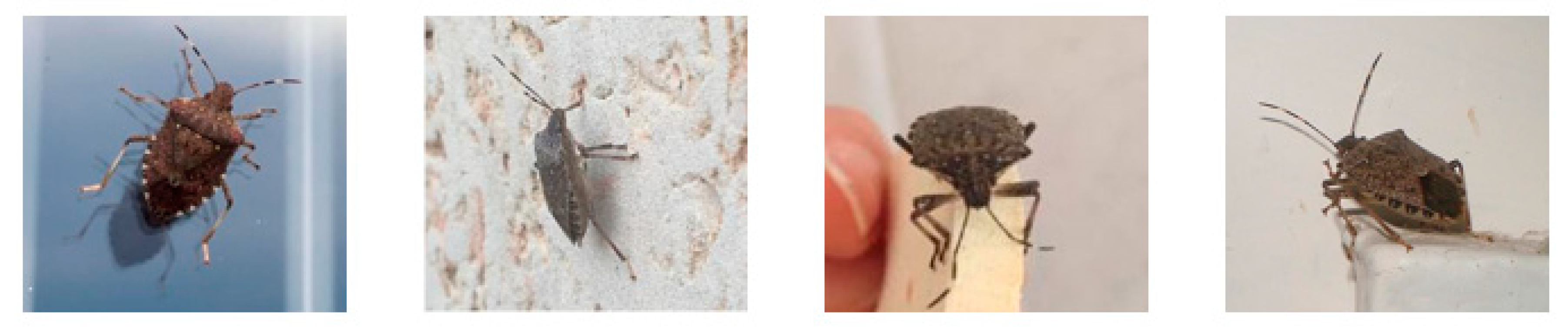
3.1. Image Collection of Citrus Pests
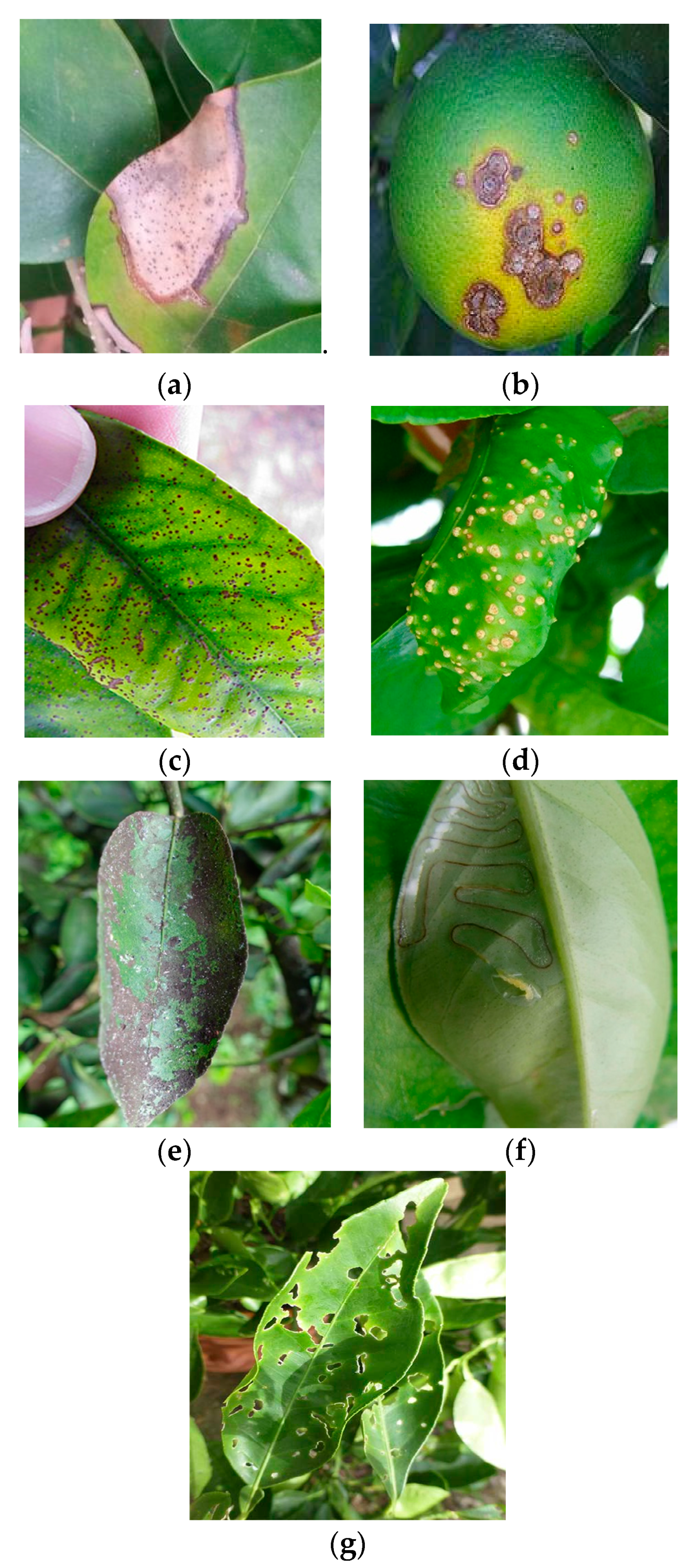
3.2. Image Collection of Citrus Diseases
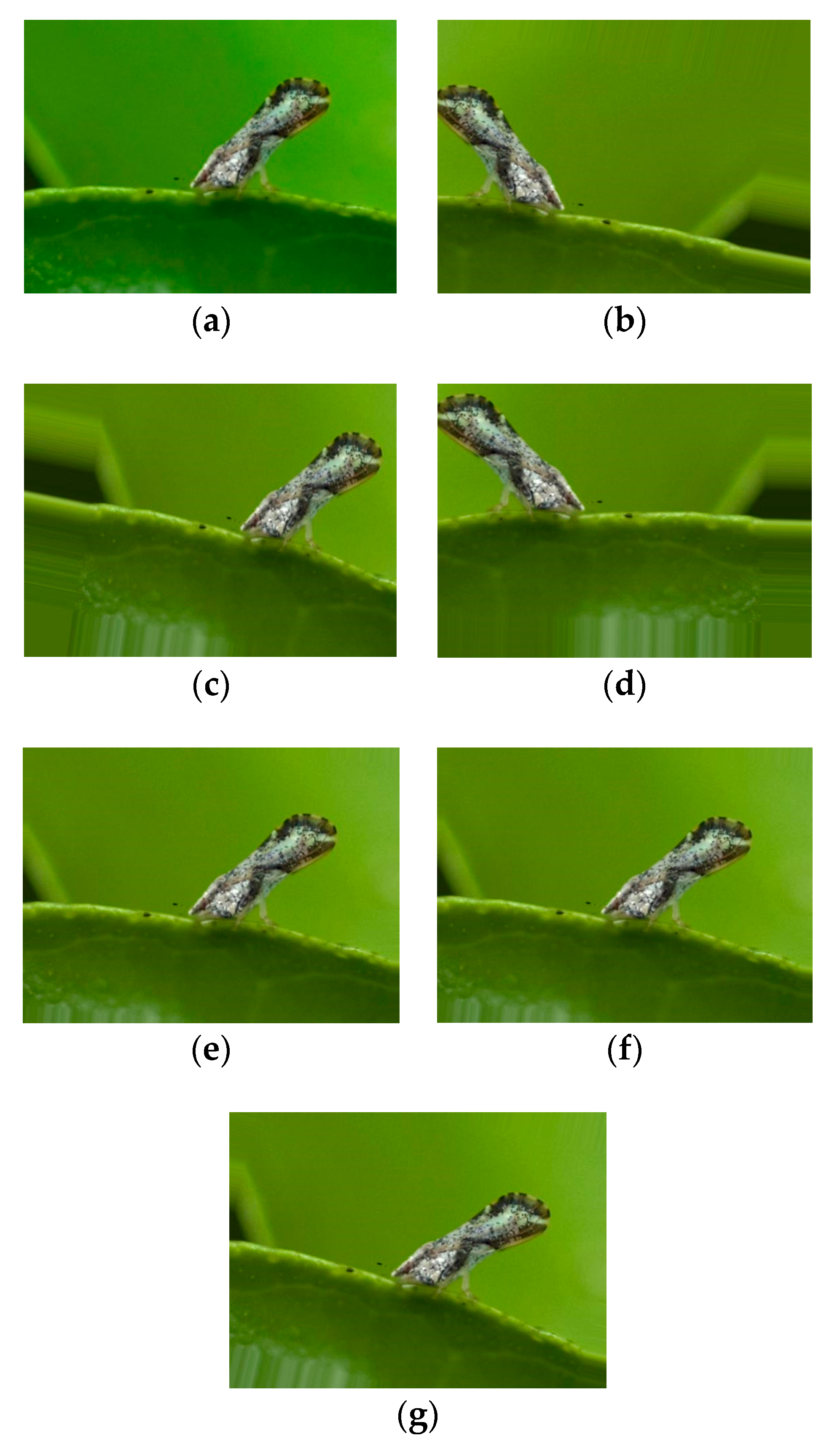
3.3. Data Augmentation
4. Weakly DenseNet Architecture
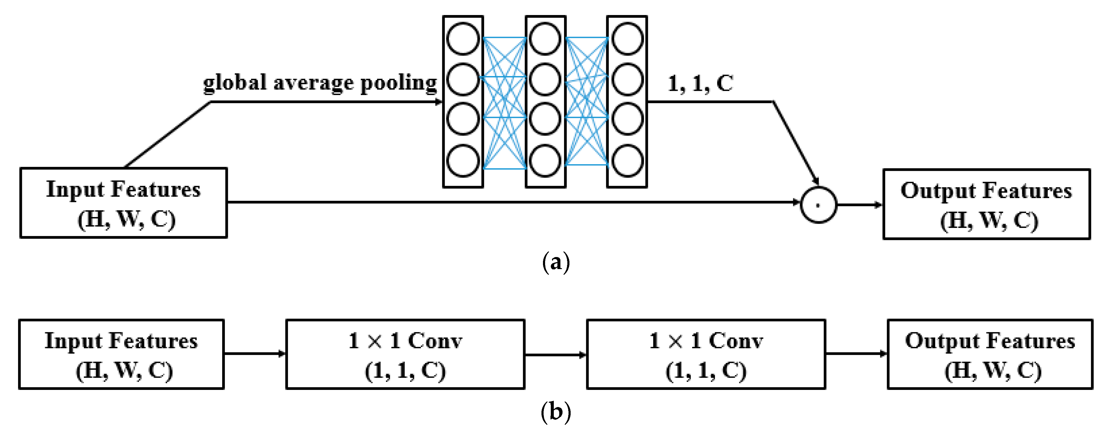
4.1. The 1 × 1 Convolution for Feature Refinement
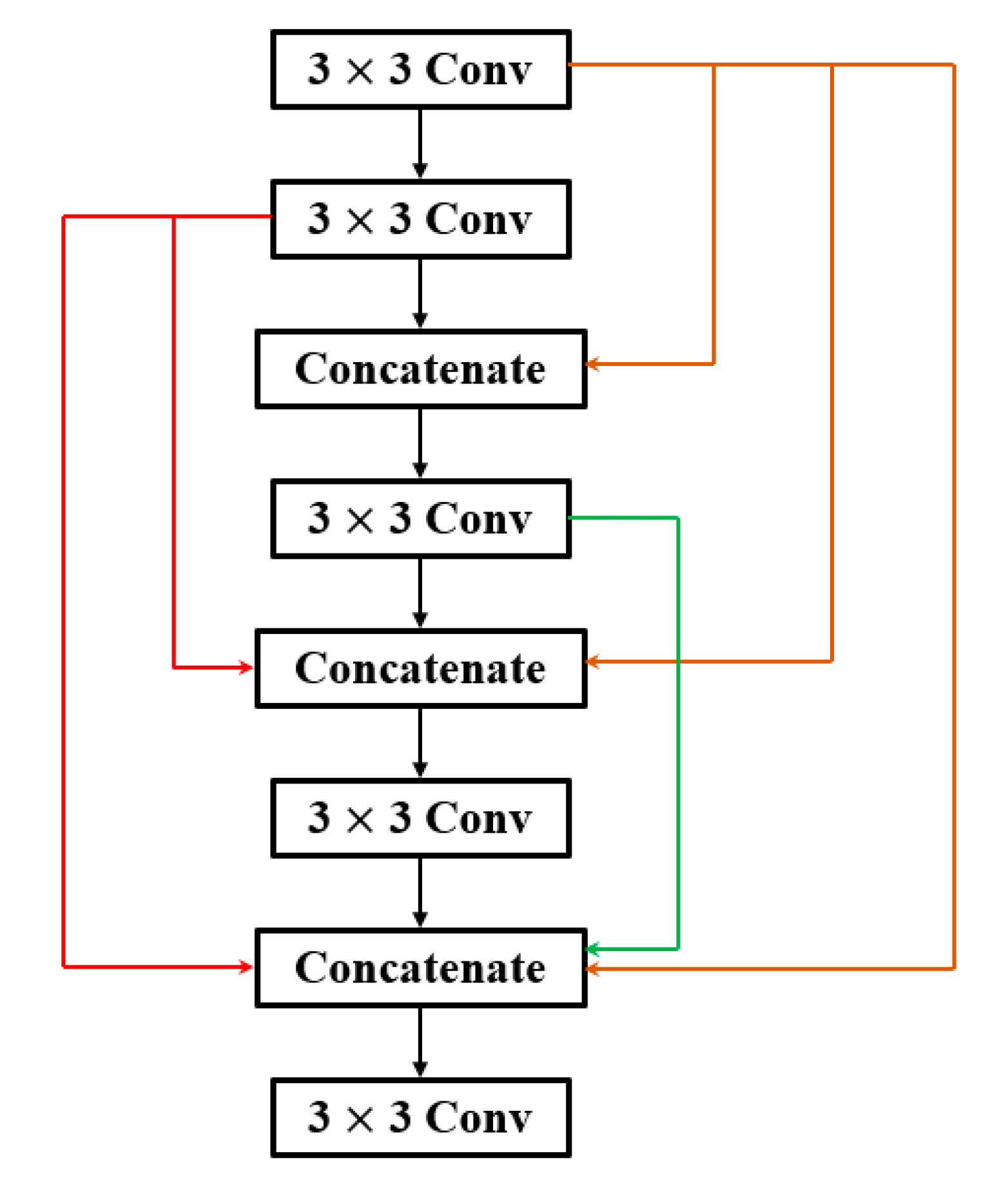
4.2. Feature Reuse
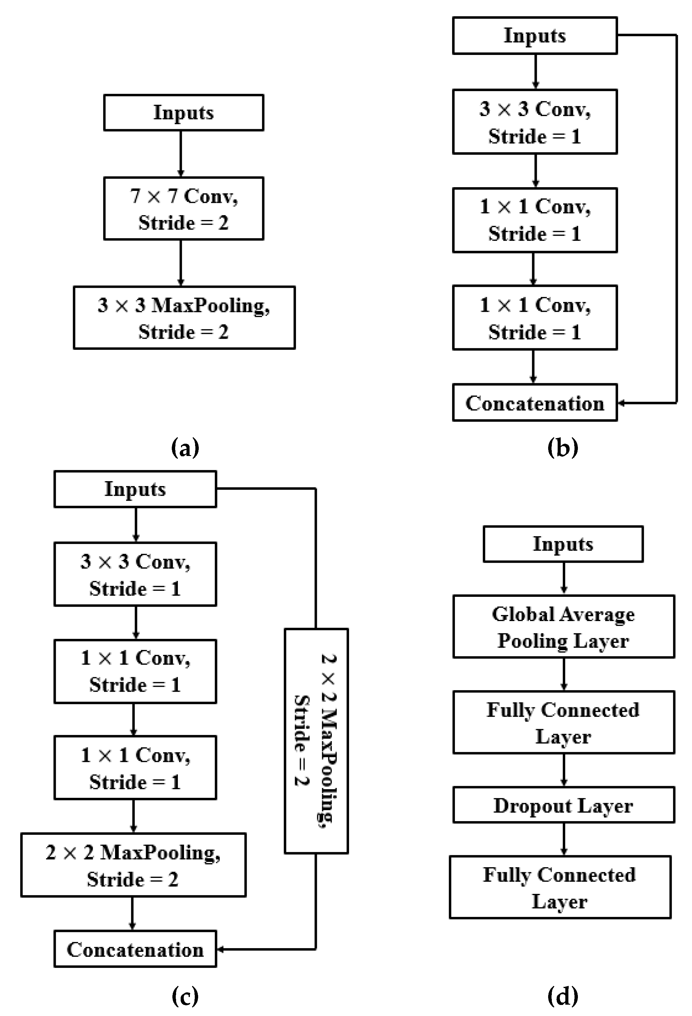
4.3. Network Architecture
5. Experiments and Results
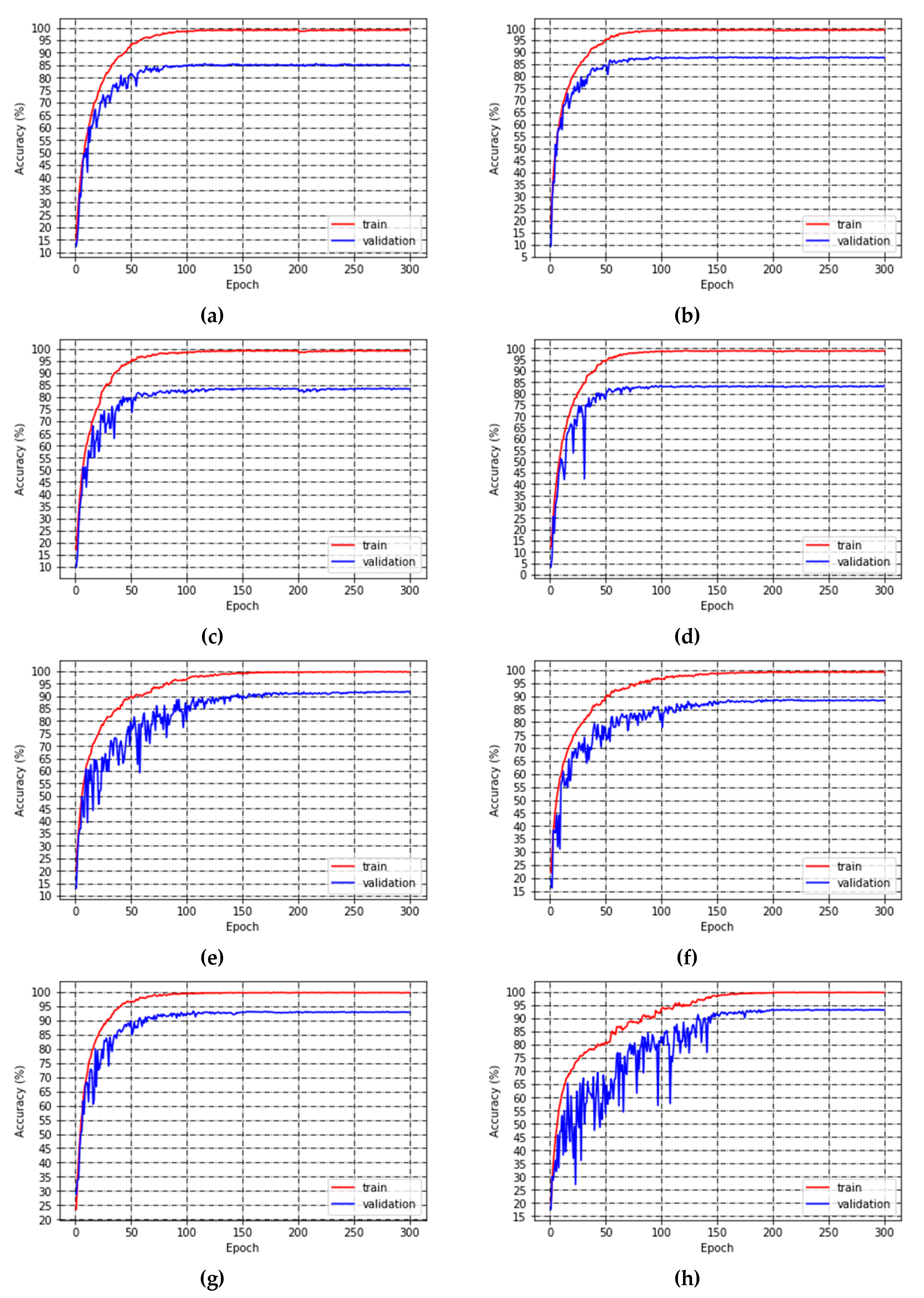
5.1. Training
| Algorithm 1. Learning Rate Schedule |
| Input: Patience P, decay , validation loss L Output: Learning rate 1: Initialize L = L0, 2: i ← 0 3: while i < P do 4: if L Li then 5: i = i + 1 6: else 7: L = Li 8: i = i + 1 9: end if 10: end while 11: if L = L0 then 12: 13: end if |
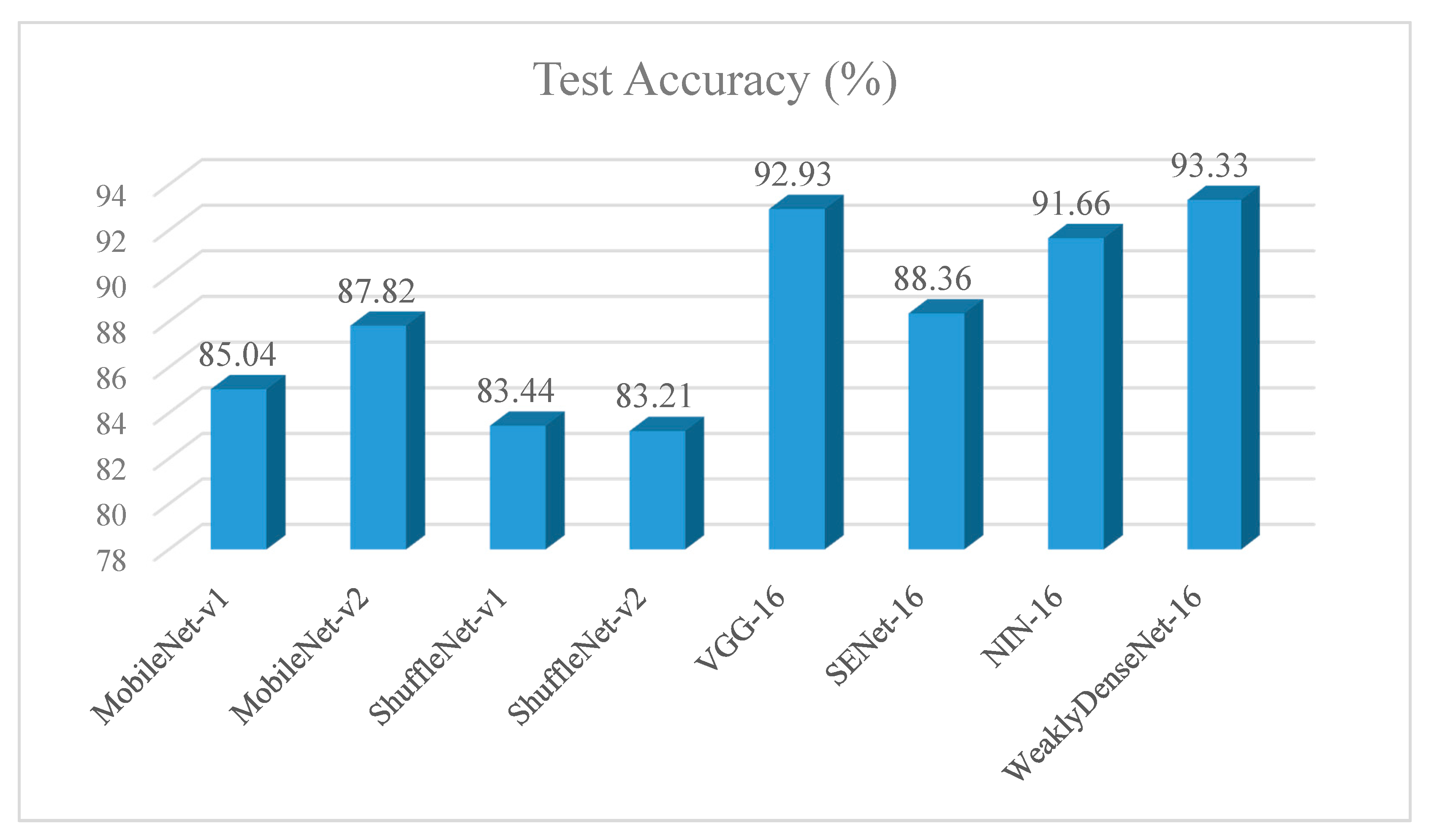
5.2. Test
6. Conclusions and Future Work
Author Contributions
Funding
Conflicts of Interest
Appendix A

Appendix B
Appendix C
References
- LeCun, Y.; Bengio, Y.; Hinton, G. Deep learning. Nature 2015, 521, 436–444. [Google Scholar] [CrossRef] [PubMed]
- Liang, Q.; Xiang, S.; Hu, Y.; Coppola, G.; Zhang, D.; Sun, W. PD2SE-Net: Computer-assisted plant disease diagnosis and severity estimation network. Comput. Electron. Agric. 2019, 157, 518–529. [Google Scholar] [CrossRef]
- Cheng, X.; Zhang, Y.; Chen, Y.; Wu, Y.; Yue, Y. Pest identification via deep residual learning in complex background. Comput. Electron. Agric. 2017, 141, 351–356. [Google Scholar] [CrossRef]
- Shen, Y.; Zhou, H.; Li, J.; Jian, F.; Jayas, D.S. Detection of stored-grain insects using deep learning. Comput. Electron. Agric. 2018, 145, 319–325. [Google Scholar] [CrossRef]
- Ren, S.Q.; He, K.M.; Girshick, R.; Sun, J. Faster R-CNN: Towards Real-Time Object Detection with Region Proposal Networks. IEEE Trans. Pattern Anal. Mach. Intell. 2017, 39, 1137–1149. [Google Scholar] [CrossRef] [PubMed]
- Szegedy, C.; Vanhoucke, V.; Ioffe, S.; Shlens, J.; Wojna, Z. Rethinking the inception architecture for computer vision. arXiv 2015, arXiv:1512.00567. [Google Scholar]
- Jeong, J.; Park, H.; Kwak, N. Enhancement of SSD by concatenating feature maps for object detection. arXiv 2017, arXiv:1705.09587. [Google Scholar]
- Zhuang, X.; Zhang, T. Detection of sick broilers by digital image processing and deep learning. Biosyst. Eng. 2019, 179, 106–116. [Google Scholar] [CrossRef]
- Deng, J.; Dong, W.; Socher, R.; Li, L.J.; Li, K.; Li, F.F. ImageNet: A large-scale hierarchical image database. In Proceedings of the IEEE Conference on Computer Vision and Pattern Recognition (CVPR), Miami, FL, USA, 20–25 June 2009. [Google Scholar]
- Reyes, A.K.; Caicedo, J.C.; Camargo, J.E. Fine—Tuning Deep Convolutional Networks for Plant Recognition. In Proceedings of the CLEF (Working Notes), Toulouse, France, 8–11 September 2015. [Google Scholar]
- Li, H.; Kadav, A.; Durdanovic, I.; Samet, H.; Graf, H.P. Pruning Filters for Efficient ConvNets. arXiv 2016, arXiv:1608.08710v3. [Google Scholar]
- Molchanov, P.; Tyree, S.; Karras, T.; Aila, T.; Kautz, J. Pruning Convolutional Neural Networks for Resource Efficient Inference. arXiv 2016, arXiv:1611.06440v2. [Google Scholar]
- Hu, J.; Shen, L.; Albanie, S.; Sun, G.; Wu, E. Squeeze-and-Excitation Networks. arXiv 2017, arXiv:1709.01507. [Google Scholar]
- Woo, S.; Park, J.; Lee, J.Y.; Kweon, I.S. CBAM: Convolutional Block Attention Module. arXiv 2018, arXiv:1807.06521. [Google Scholar]
- Srivastava, N.; Hinton, G.; Krizhevsky, A.; Sutskever, I.; Salakhutdinov, R. Dropout: A simple way to prevent neural networks from overfitting. J. Mach. Learn. Res. 2014, 15, 1929–1958. [Google Scholar]
- Huang, G.; Sun, Y.; Liu, Z.; Sedra, D.; Weinberger, K. Deep Networks with Stochastic Depth. arXiv 2016, arXiv:1603.09382v3. [Google Scholar]
- Lin, M.; Chen, Q.; Yan, S. Network in network. arXiv 2013, arXiv:1312.4400v3. [Google Scholar]
- Srivastava, R.K.; Greff, K.; Schmidhuber, J. Highway Networks. arXiv 2015, arXiv:1505.00387. [Google Scholar]
- He, K.; Zhang, X.; Ren, S.; Sun, J. Deep residual learning for image recognition. arXiv 2015, arXiv:1512.03385. [Google Scholar]
- Huang, G.; Liu, Z.; van der Maaten, L.; Weinberger, K.Q. Densely Connected Convolutional Networks. arXiv 2016, arXiv:1608.06993v5. [Google Scholar]
- Boniecki, P.; Koszela, K.; Piekarska Boniecki, H.; Weres, M.; Zaborowcz, M.; Kujawa, A.; Majewski, A.; Raba, B. Neural identification of selected apple pests. Comput. Electron. Agric. 2015, 110, 9–16. [Google Scholar] [CrossRef]
- Sun, Y.; Jiang, Z.; Zhang, L.; Dong, W.; Rao, Y. SLIC_SVM based leaf diseases saliency map extraction of tea plant. Comput. Electron. Agric. 2019, 157, 102–109. [Google Scholar] [CrossRef]
- Ferentinos, K.P. Deep learning models for plant disease detection and diagnosis. Comput. Electron. Agric. 2018, 145, 311–318. [Google Scholar] [CrossRef]
- Simonyan, K.; Zisserman, A. Very deep convolutional networks for large-scale image recognition. arXiv 2014, arXiv:1409.1556. [Google Scholar]
- Zagoruyko, S.; Komodakis, N. Wide residual networks. In Proceedings of the British Machine Vision Conference (BMVC), York, UK, 19–22 September 2016. [Google Scholar]
- Lee, C.Y.; Xie, S.; Gallagher, P.; Zhang, Z.; Tu, Z. Deeply-supervised nets. In Proceedings of the 18th International Conference on Artificial Intelligence and Statistics, San Diego, CA, USA, 9–12 May 2015. [Google Scholar]
- Chollet, F. Xception: Deep Learning with Depthwise Separable Convolutions. In Proceedings of the 30th IEEE Conference on Computer Vision and Pattern Recognition (CVPR), Honolulu, HI, USA, 22–25 July 2017. [Google Scholar]
- Howard, A.G.; Zhu, M.; Chen, B.; Kalenichenko, D.; Wang, W.; Weyand, T.; Andreetto, M.; Adam, H. MobileNets: Efficient Convolutional Neural Networks for Mobile Vision Applications. arXiv 2017, arXiv:704.04861. [Google Scholar]
- Sandler, M.; Howard, A.; Zhu, M.; Zhmoginov, A.; Chen, L. MobileNetV2: Inverted Residuals and Linear Bottlenecks. arXiv 2018, arXiv:1801.04381v4. [Google Scholar]
- Zhang, X.; Zhou, X.; Lin, M.; Sun, J. ShuffleNet: An Extremely Efficient Convolutional Neural Network for Mobile Devices. arXiv 2017, arXiv:1707.01083. [Google Scholar]
- Ma, N.; Zhang, X.; Zheng, H.; Sun, J. ShuffleNet V2: Practical Guidelines for Efficient CNN Architecture Design. arXiv 2018, arXiv:1807.11164. [Google Scholar]
- Nair, V.; Hinton, G.E. Rectified linear units improve restricted boltzmann machines. In Proceedings of the 27th International Conference on Machine Learning (ICML), Haifa, Israel, 21–24 June 2010. [Google Scholar]
- Xie, S.; Girshick, R.; Dollar, P.; Tu, Z.; He, K. Aggregated Residual Transformations for Deep Neural Networks. arXiv 2016, arXiv:1611.05431. [Google Scholar]
- Das, S.; Datta, S.; Chaudhuri, B.B. Handling data irregularities in classification: Foundations, trends, and future challenges. Pattern Recognit. 2018, 81, 674–693. [Google Scholar] [CrossRef]
- Yosinski, J.; Clune, J.; Bengio, Y.; Lipson, H. How transferable are features in deep neural networks? In Proceedings of the 28th International Conference on Neural Information Processing Systems (NeurIPS), Montreal, PQ, Canada, 8–13 December 2014. [Google Scholar]
- Ioffe, S.; Szegedy, C. Batch normalization: Accelerating deep network training by reducing internal covariate shift. arXiv 2015, arXiv:1502.03167. [Google Scholar]
- Sutskever, I.; Martens, J.; Dahl, G.E.; Hinton, G.E. On the importance of initialization and momentum in deep learning. In Proceedings of the 30th International Conference on Machine Learning (ICML), Atlanta, GA, USA, 16–21 June 2013. [Google Scholar]
- Masters, D.; Luschi, C. Revisiting Small Batch Training for Deep Neural Networks. arXiv 2018, arXiv:1804.07612. [Google Scholar]
- He, K.; Zhang, X.; Ren, S.; Sun, J. Delving Deep into Rectifiers: Surpassing Human-Level Performance on ImageNet Classification. In Proceedings of the 2015 International Conference on Computer Vision (ICCV), Santiago, Chile, 11–18 December 2015. [Google Scholar]
- Zeiler, M.; Fergus, R. Visualizing and Understanding Convolutional Networks. arXiv 2013, arXiv:1311.2901. [Google Scholar]


| Class ID | Common Name | Scientific Name | Number of Samples |
|---|---|---|---|
| Citrus Pests | |||
| 8 | Mediterranean fruit fly | Ceratitis capitata | 558 |
| 0 | Asian citrus psyllid | Diaphorina citri Kuwayama | 359 |
| 5 | Citrus longicorn beetle | Anoplophora chinensis | 597 |
| 7 | Brown marmorated stink bug | Halyomorpha halys | 606 |
| 3 | Southern green stink bug | Nezara viridula | 488 |
| 4 | Fruit sucking moth | Othreis fullonica | 600 |
| 1 | Citrus swallowtail | Papilio demodocus | 600 |
| 15 | Citrus flatid planthopper | Metcalfa pruinosa (Say) | 555 |
| 9 | Citrus mealybug | Planococcus citri | 495 |
| 13 | Aphids | Toxoptera citricida | 514 |
| 11 | Citrus soft scale | Hemiptera: Coccidae | 497 |
| 12 | False codling moth | Thaumatotibia leucotreta | 511 |
| 14 | Root weevil | Diaprepes abbreviatus, Pachnaeus opalus | 378 |
| 2 | Forktailed bush katydid | Scudderia furcata | 600 |
| 10 | Cicada | Cicadoidea | 508 |
| 6 | Garden snail | Cornu aspersum | 618 |
| 16 | Glassy-winged sharpshooter | Homalodisca vitripennis | 567 |
| Total | 9051 | ||
| Citrus Diseases | |||
| 17 | Anthracnose | Colletotrichum gloeosporioides | 467 |
| 18 | Canker | Xanthomonas axonopodis | 598 |
| 20 | Melanose | Diaporthe citri | 532 |
| 21 | Scab | Elsinoë fawcettii | 503 |
| 19 | Leaf miner | Liriomyza brassicae | 427 |
| 22 | Sooty mold | Capnodium spp | 568 |
| 23 | Pest hole | 415 | |
| Total | 3510 | ||
| Operation | Value |
|---|---|
| Rotation | [, ] |
| Width shift | [0, 0.2] |
| Height shift | [0, 0.2] |
| Shear | [0, 0.2] |
| Zoom | [0.8, 1.2] |
| Horizontal flip | - |
| Block | Output Size |
|---|---|
| Initial Block (a) | 56 56 32 |
| Intermediate Block (b) | 56 56 96 |
| Intermediate Block (c) | 28 28 192 |
| Intermediate Block (b) | 28 28 384 |
| Intermediate Block (c) | 14 14 768 |
| 1 1 conv, stride 1 | 14 14 512 |
| 1 1 conv, stride 1 | 14 14 512 |
| 2 2 max pool, stride 2 | 7 7 512 |
| Classification Block (d) | 1 1 24 |
| Model Name | Training Accuracy | Validation Accuracy | Model Size (MB) | Training Time (ms)/Batch Size |
|---|---|---|---|---|
| MobileNet-v1 | 99.23 | 85.45 | 25 | 152 |
| MobileNet-v2 | 99.28 | 87.97 | 33.9 | 198 |
| ShuffleNet-v1 | 99.13 | 83.58 | 28.8 | 145 |
| ShuffleNet-v2 | 98.72 | 83.58 | 42 | 144 |
| VGG-16 | 99.82 | 93 | 120.2 | 303 |
| SENet-16 | 99.10 | 88.71 | 19.5 | 138 |
| NIN-16 | 99.63 | 91.84 | 19.6 | 137 |
| WeaklyDenseNet-16 | 99.83 | 93.42 | 30.5 | 138 |
© 2019 by the authors. Licensee MDPI, Basel, Switzerland. This article is an open access article distributed under the terms and conditions of the Creative Commons Attribution (CC BY) license (http://creativecommons.org/licenses/by/4.0/).
Share and Cite
Xing, S.; Lee, M.; Lee, K.-k. Citrus Pests and Diseases Recognition Model Using Weakly Dense Connected Convolution Network. Sensors 2019, 19, 3195. https://doi.org/10.3390/s19143195
Xing S, Lee M, Lee K-k. Citrus Pests and Diseases Recognition Model Using Weakly Dense Connected Convolution Network. Sensors. 2019; 19(14):3195. https://doi.org/10.3390/s19143195
Chicago/Turabian StyleXing, Shuli, Marely Lee, and Keun-kwang Lee. 2019. "Citrus Pests and Diseases Recognition Model Using Weakly Dense Connected Convolution Network" Sensors 19, no. 14: 3195. https://doi.org/10.3390/s19143195
APA StyleXing, S., Lee, M., & Lee, K.-k. (2019). Citrus Pests and Diseases Recognition Model Using Weakly Dense Connected Convolution Network. Sensors, 19(14), 3195. https://doi.org/10.3390/s19143195