Measurement and Characterization of Electromagnetic Noise in Edge Computing Networks for the Industrial Internet of Things

Abstract
:1. Introduction
2. Measurement Environments and Methods
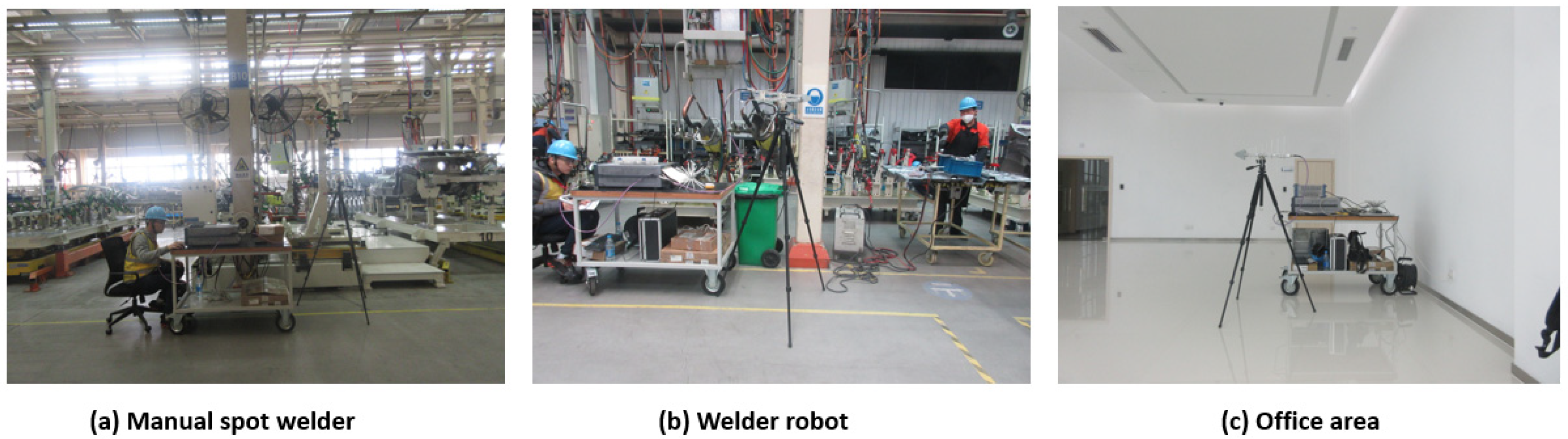
2.1. Measurement Positions
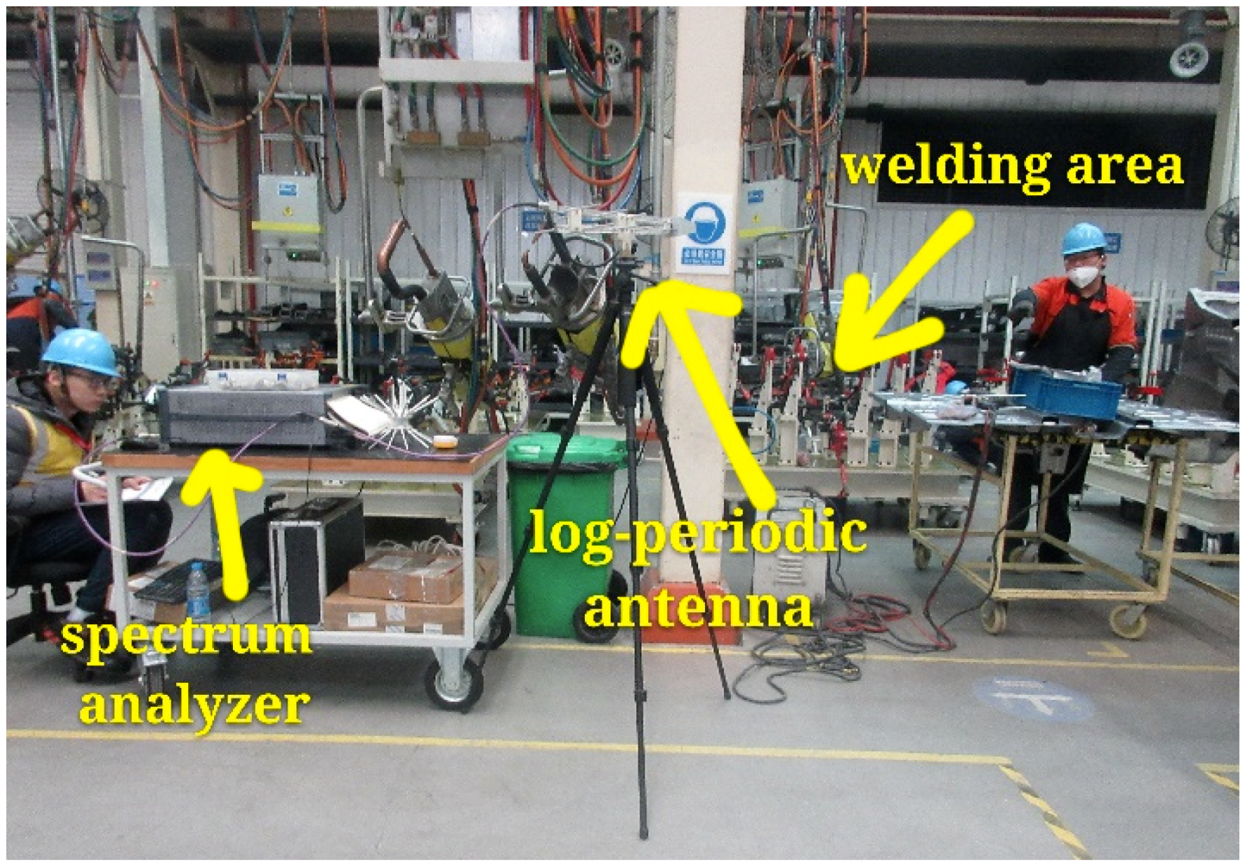
2.2. Measurement Equipment
2.3. Frequency Domain Measurement Method
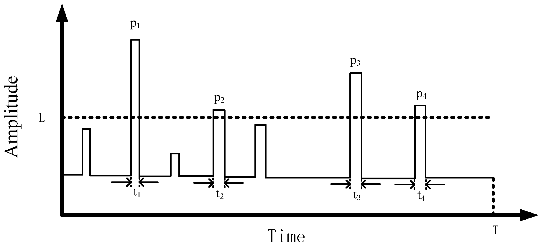
2.4. Time Domain Measurement Method
3. Statistical Parameters
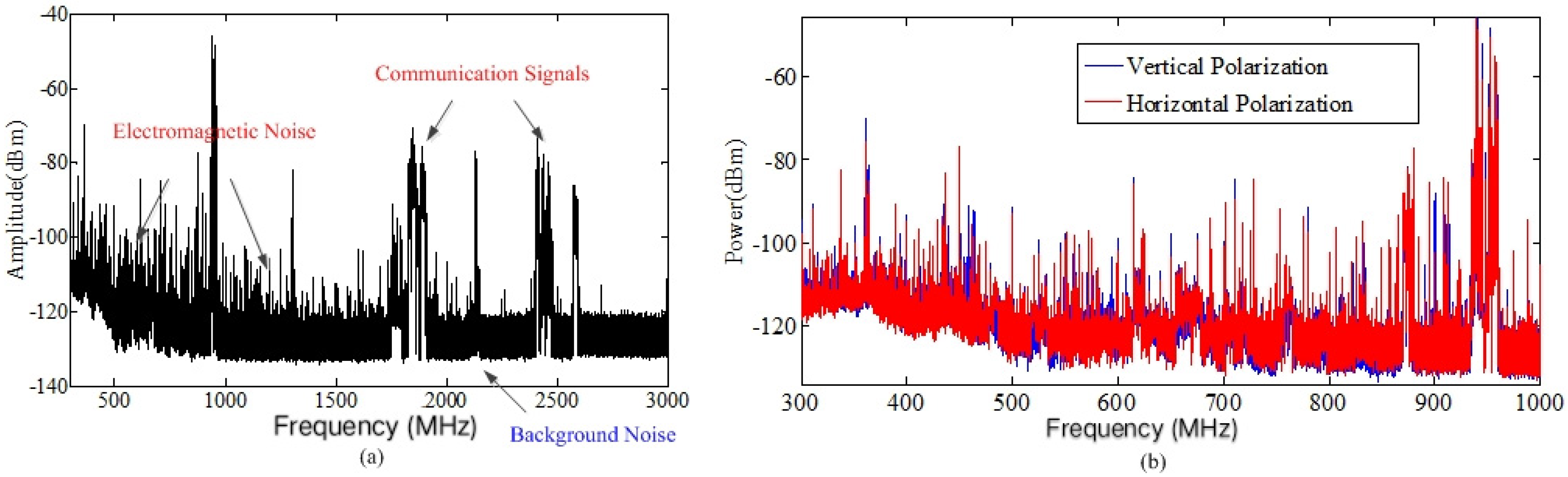
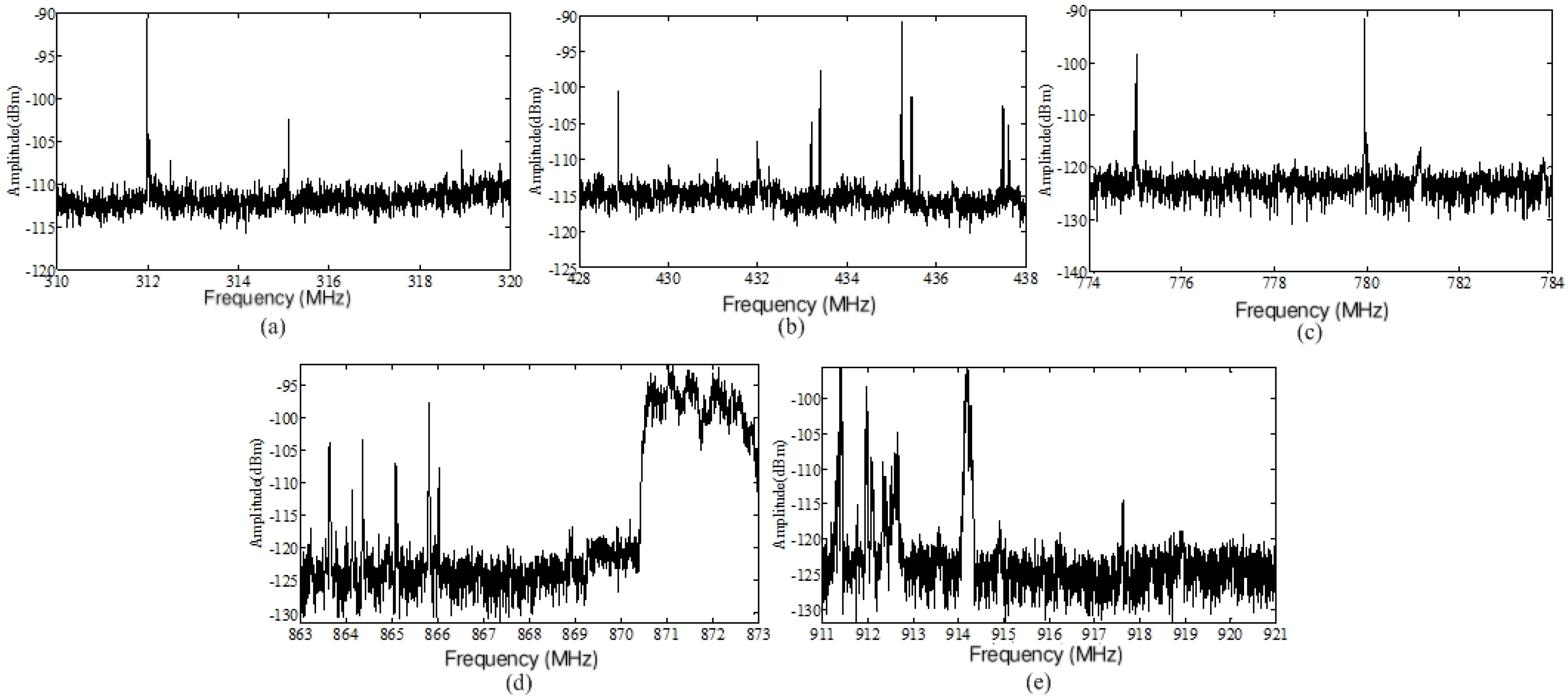
4. Characterization Using the Frequency Domain Measurement Data
5. Characterization Using the Time Domain Measurement Data
5.1. Measurement Results
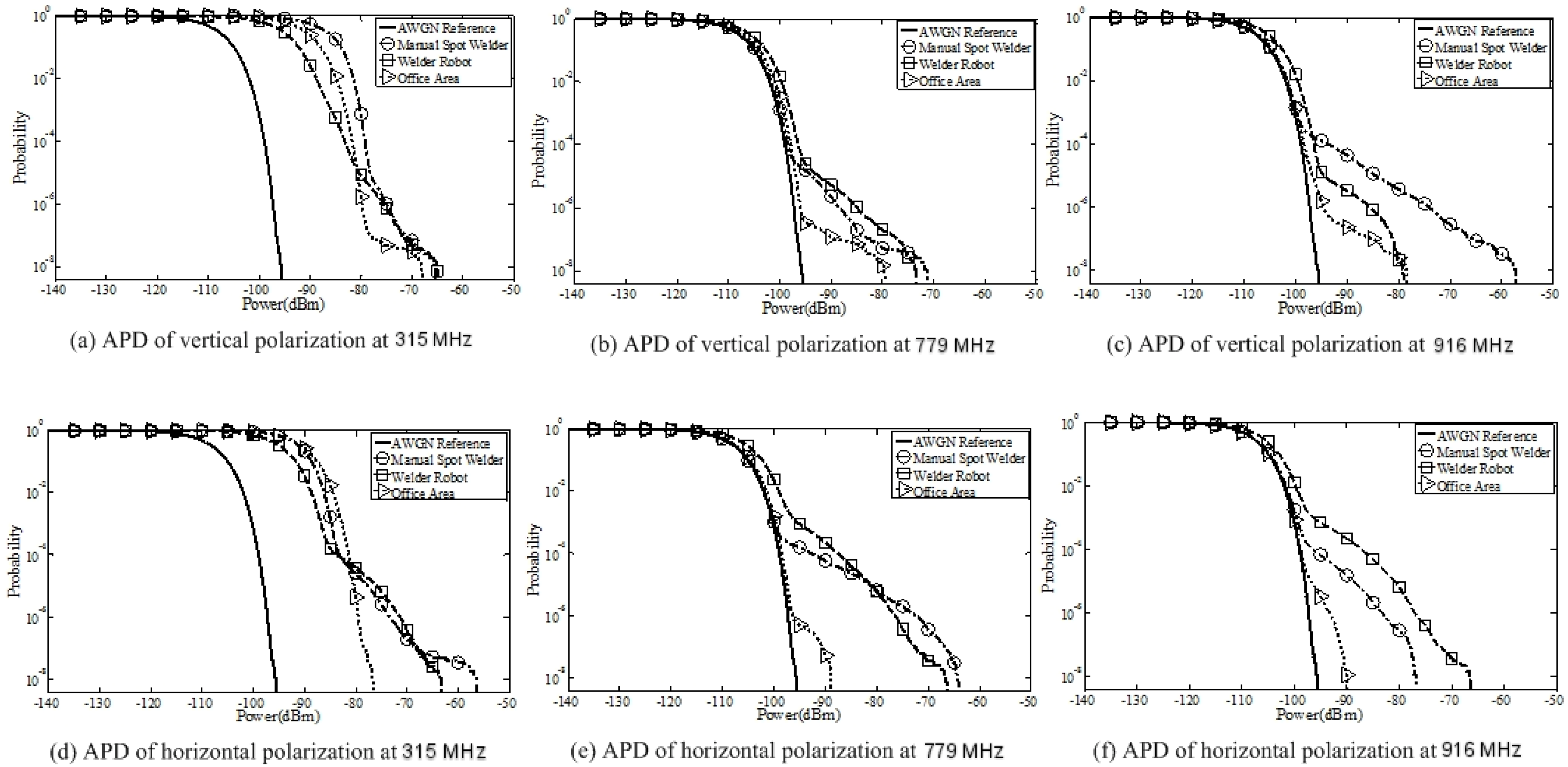
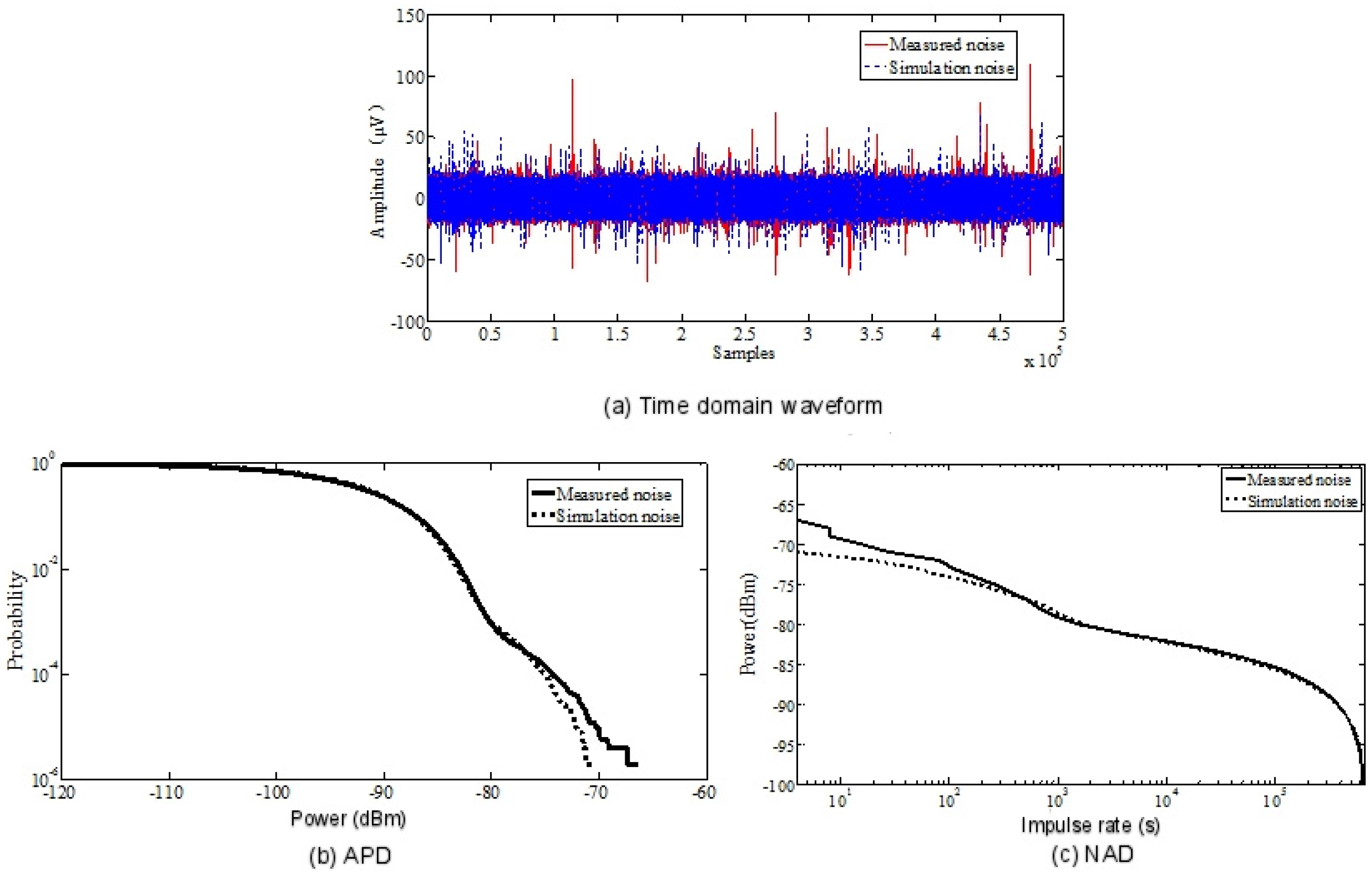
5.1.1. APD Results
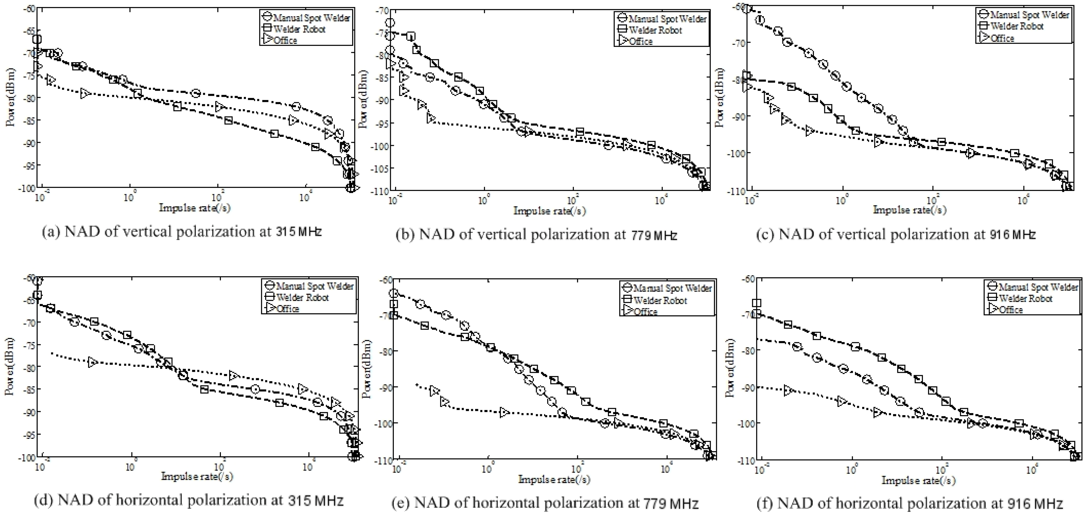
5.1.2. NAD Results
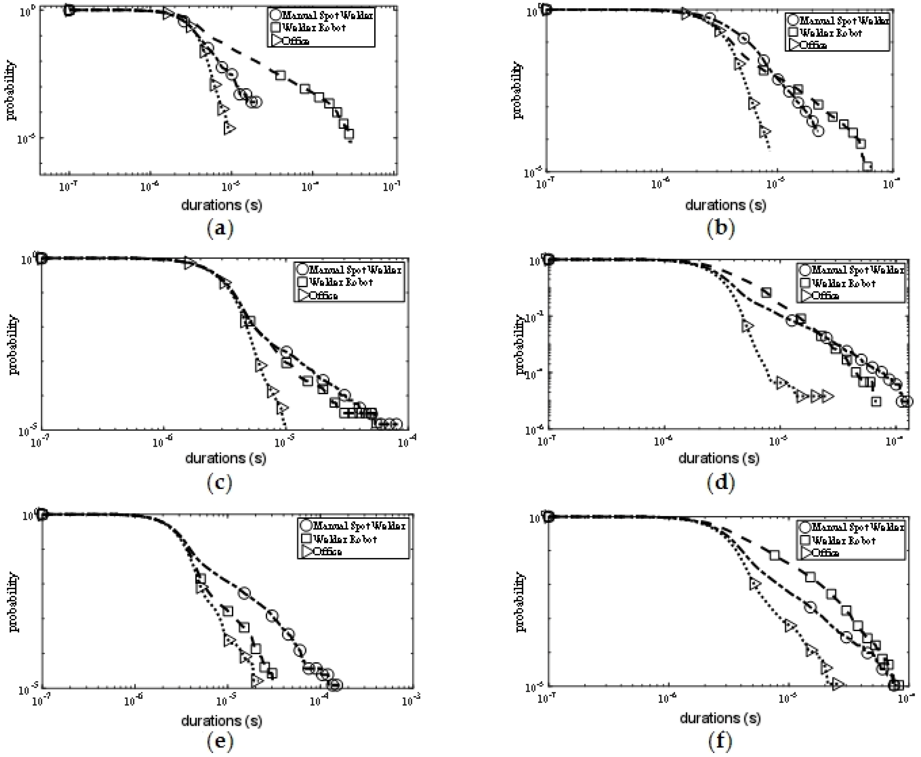
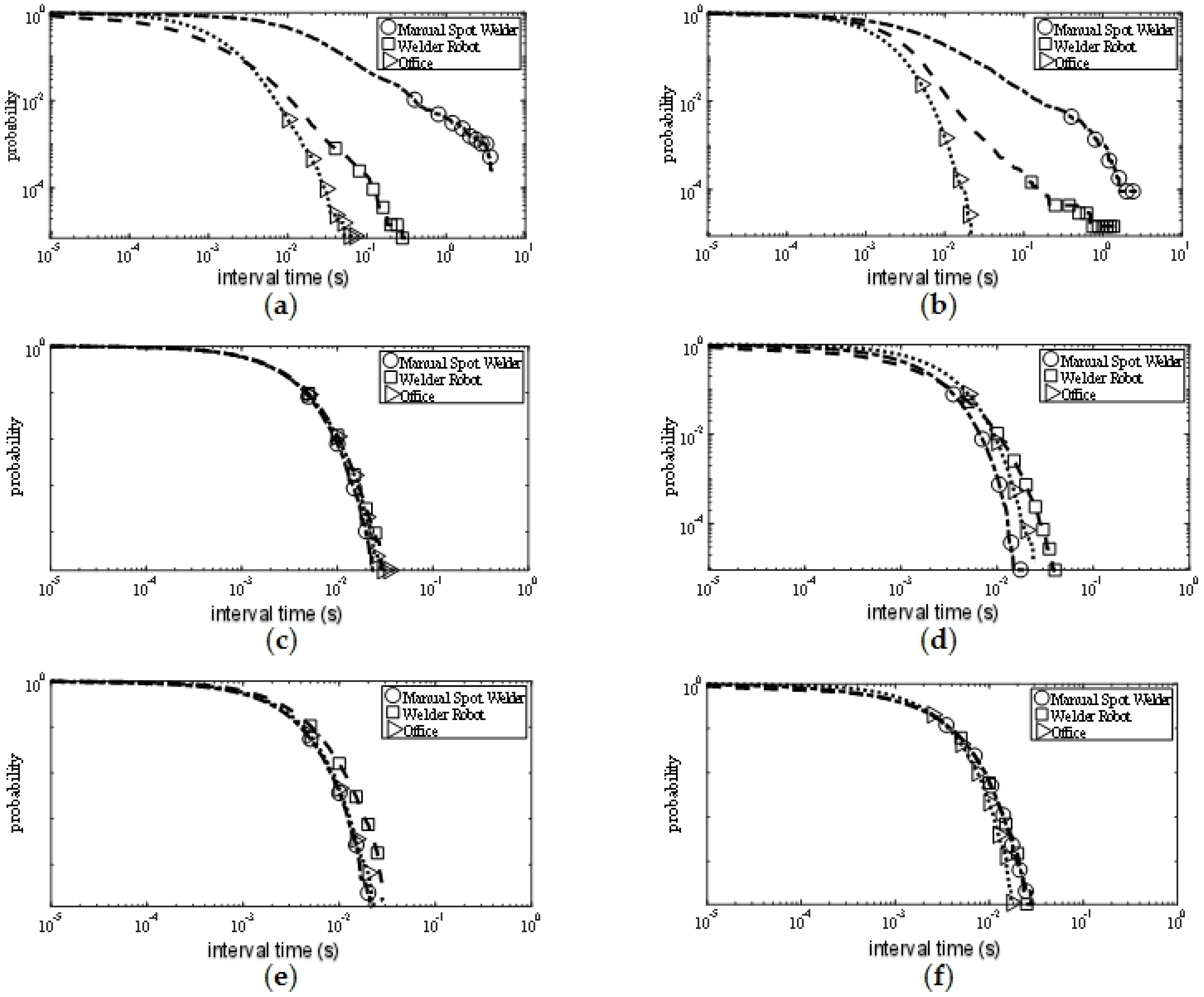
5.1.3. PDD Results
5.1.4. PSD Results
5.2. Modeling of Time-Varying Characteristics
5.2.1. CHMM Definition
5.2.2. CHMM Modeling Method
6. Conclusions
Author Contributions
Funding
Conflicts of Interest
References
- Wan, J.; Yi, M.; Li, D.; Zhang, C.; Wang, S.; Zhou, K. Mobile Services for Customization Manufacturing Systems: An Example of Industry 4.0. IEEE Access 2016, 4, 8977–8986. [Google Scholar] [CrossRef]
- Li, X.; Li, D.; Wan, J.; Vasilakos, A.V.; Lai, C.F.; Wang, S. A review of industrial wireless networks in the context of Industry 4.0. Wirel. Netw. 2017, 23, 23–41. [Google Scholar] [CrossRef]
- Wan, J.; Tang, S.; Shu, Z.; Li, D.; Wang, S.; Imran, M.; Vasilakos, A.V. Software-Defined Industrial Internet of Things in the Context of Industry 4.0. IEEE Sens. J. 2016, 16, 7373–7380. [Google Scholar] [CrossRef]
- Fernández-Caramés, T.M.; Fraga-Lamas, P.; Suárez-Albela, M.; Díaz-Bouza, M.A. A Fog Computing Based Cyber-Physical System for the Automation of Pipe-Related Tasks in the Industry 4.0 Shipyard. Sensors 2018, 18, 1961. [Google Scholar] [CrossRef] [PubMed]
- Lavassani, M.; Forsström, S.; Jennehag, U.; Zhang, T. Combining Fog Computing with Sensor Mote Machine Learning for Industrial IoT. Sensors 2018, 18, 1532. [Google Scholar] [CrossRef] [PubMed]
- Delsing, J. Local cloud internet of things automation: Technology and business model features of distributed internet of things automation solutions. IEEE Ind. Electron. Mag. 2017, 11, 8–21. [Google Scholar] [CrossRef]
- Wang, H. The Application of Edge Computing in Smart City. Comput. Fan 2018, 8, 138. [Google Scholar]
- Mumtaz, S.; Ai, B.; Al-Dulaimi, A.; Tsang, K.-F. 5G and beyond mobile technologies and applications for industrial IoT (IIoT). IEEE Trans. Ind. Inf. 2018, 14, 2588–2591. [Google Scholar] [CrossRef]
- Cheffena, M. Propagation channel characteristics of industrial wireless sensor networks. IEEE Antennas Propag. Mag. 2016, 58, 66–73. [Google Scholar] [CrossRef]
- Stenumgaard, P.; Chilo, J.; Ferrer-Coll, P.; Angskog, P. Challenges and conditions for wireless machine-to-machine communications in industrial environments. Commun. Mag. IEEE 2013, 51, 187–192. [Google Scholar] [CrossRef]
- Zhang, K. Research on Broadband Channel Measurement and Fading Characteristics of Industrial Internet of Things; Institute of Broadband Wireless Communications, Beijing Jiaotong University: Beijing, China, 2018; pp. 9–10. [Google Scholar]
- Liu, L.; Zhang, K.; Tian, L.; Zhou, T.; Tao, C.; Chen, H.; Lou, J. Realistic Channel Modeling for Industrial. Internet Things 2018, 11, 13–14. [Google Scholar]
- Mumtaz, S.; Alsohaily, A.; Pang, Z.; Rayes, A.; Fung-Tsang, K.; Rodriguez, J. Massive Internet of things for industrial applications: Addressing wireless IIoT connectivity challenges and ecosystem fragmentation. IEEE Ind. Electron. Mag. 2017, 11, 28–33. [Google Scholar] [CrossRef]
- Cheffena, M. Industrial wireless sensor networks: Channel modeling and performance evaluation. EURASIP J. Wirel. Commun. Netw. 2012, 2012, 1–8. [Google Scholar] [CrossRef]
- Coll J, F.; Chilo, J.; Slimane, B. Radio-Frequency electromagnetic characterization in factory infrastructures. IEEE Trans. Electromagn. Compat. 2012, 54, 708–711. [Google Scholar] [CrossRef]
- Saaifan, K.A.; Henkel, W. Measurements and modeling of impulse noise at the 2.4 GHz wireless LAN band. Signal Inf. Process. IEEE 2018, 11, 86–90. [Google Scholar]
- Blankenship, T.K.; Kriztman, D.M.; Rappaport, T.S. Measurements and simulation of radio frequency impulsive noise in hospitals and clinics. In Proceedings of the 47th IEEE Vehicular Technology Conference, Phoenix, AZ, USA, 4–7 May 1997. [Google Scholar]
- Chilo, J.; Karlsson, C.; Angskog, P.; Stenumgaard, P. Impulsive noise measurement methodologies for APD determination in M2M environments. IEEE Int. Symp. Electromagn. Compat. 2009, 50, 151–154. [Google Scholar]
- Zhang, J.; Lu, Y.; Xu, D.; Liu, G.; Zhang, P.; Huang, Y. Method and Apparatus for Noise Floor and Signal Component Threshold Estimation Based on Channel Measurement. CN Patent CN101426212, 6 May 2009. [Google Scholar]
- Rhee, J.G. Statistical analysis of radio frequency noise spectrum in Korea. Int. Symp. Electromagn. Compat. 1999, 11, 193–196. [Google Scholar]
- Chang, M.H.; Lin, K.H. A comparative investigation on urban radio noise at several specific measured areas and its applications for communications. IEEE Trans. Broadcast. 2004, 50, 233–243. [Google Scholar] [CrossRef]
- Rabiner, L.R.; Juang, B.H.; Levinson, S.E.; Sondhi, M.M. Some Properties of Continuous Hidden Markov Model Representations. Bell Labs Tech. J. 1985, 64, 1251–1270. [Google Scholar] [CrossRef]
- Vaseghi, S.V. Advanced Digital Signal Processing and Noise Reduction, 4th ed.; John Wiley & Sons, Inc.: Hoboken, NJ, USA, 2009. [Google Scholar]
- Sanchez, M.G.; De Haro, L.; Ramon, M.C.; Mansilla, A.; Montero Ortega, C.; Oliver, D. Impulsive noise measurements and characterization in a UHF digital TV channel. Trans. Electromagn. Compat. IEEE 1999, 41, 124–136. [Google Scholar] [CrossRef]


| Parameters | Values |
|---|---|
| Frequency Band | 300 MHz–3 GHz |
| Mode | Occupied BW |
| Span | 50 MHz |
| RBW(Resolution Bandwidth) | 10 kHz |
| VBW(Video Bandwidth) | 100 kHz |
| Attenuation | 2 dB |
| Preamp | Open |
| Points | 20001 |
| Polarized | Vertically/Horizontally |
| Parameters | Values |
|---|---|
| Frequency | 315 MHz, 779 MHz, 916 MHz |
| Bandwidth | 200 kHz |
| Sampling Rate | 2 MHz |
| Measurement Duration | 134.2 s |
| Mode | Data Collecting |
| Polarized | Vertically/Horizontally |
| Frequency (MHz) | Signal Type | Frequency (MHz) | Signal Type |
|---|---|---|---|
| 478–486 | Radio and TV Signals | 825–835 | CDMA UL |
| 518–526 | 870–880 | CDMA DL | |
| 526–534 | 890–915 | GSM800 UL | |
| 614–622 | 935–960 | GSM800 DL | |
| 654–662 | 1710–1755 | GSM1800 UL | |
| 662–670 | 1755–1785 | FDD-LTE UL | |
| 670–678 | 1805–1840 | GSM1800 DL | |
| 702–710 | 1840–1875 | FDD-LTE DL | |
| 718–726 | 1885–1915 | TD-LTE | |
| 758–766 | 2130–2145 | WCDMA DL | |
| 766–774 | 2401–2481 | WIFI | |
| 790–798 | 2575–2595 | TD-LTE |
| Frequency (MHz) | 315 | 433 | 779 | 868 | 916 |
|---|---|---|---|---|---|
| Average power of noise (dBm) | −111.0 | −113.5 | −118.3 | −119.3 | −124.1 |
| Frequency (MHz) | 315 | 433 | 779 | 868 | 916 |
|---|---|---|---|---|---|
| Path Loss (dB) | 62.4 | 65.2 | 70.3 | 71.2 | 71.7 |
| Frequency (MHz) | 315 | 433 | 779 | 868 | 916 |
|---|---|---|---|---|---|
| Gain (dB) | 0 | −0.3 | −0.6 | −0.5 | 3.8 |
© 2019 by the authors. Licensee MDPI, Basel, Switzerland. This article is an open access article distributed under the terms and conditions of the Creative Commons Attribution (CC BY) license (http://creativecommons.org/licenses/by/4.0/).
Share and Cite
Li, H.; Liu, L.; Li, Y.; Yuan, Z.; Zhang, K. Measurement and Characterization of Electromagnetic Noise in Edge Computing Networks for the Industrial Internet of Things. Sensors 2019, 19, 3104. https://doi.org/10.3390/s19143104
Li H, Liu L, Li Y, Yuan Z, Zhang K. Measurement and Characterization of Electromagnetic Noise in Edge Computing Networks for the Industrial Internet of Things. Sensors. 2019; 19(14):3104. https://doi.org/10.3390/s19143104
Chicago/Turabian StyleLi, Huiting, Liu Liu, Yiqian Li, Ze Yuan, and Kun Zhang. 2019. "Measurement and Characterization of Electromagnetic Noise in Edge Computing Networks for the Industrial Internet of Things" Sensors 19, no. 14: 3104. https://doi.org/10.3390/s19143104
APA StyleLi, H., Liu, L., Li, Y., Yuan, Z., & Zhang, K. (2019). Measurement and Characterization of Electromagnetic Noise in Edge Computing Networks for the Industrial Internet of Things. Sensors, 19(14), 3104. https://doi.org/10.3390/s19143104