Review

Compressed Sensing Radar Imaging: Fundamentals, Challenges, and Advances

College of Electronic Science and Technology, National University of Defense Technology, Changsha 410073, China
*
Author to whom correspondence should be addressed.
Sensors 2019, 19(14), 3100; https://doi.org/10.3390/s19143100
Submission received: 3 June 2019 / Revised: 8 July 2019 / Accepted: 11 July 2019 / Published: 13 July 2019
(This article belongs to the Special Issue Recent Advancements in Radar Imaging and Sensing Technology)

Abstract

:
In recent years, sparsity-driven regularization and compressed sensing (CS)-based radar imaging methods have attracted significant attention. This paper provides an introduction to the fundamental concepts of this area. In addition, we will describe both sparsity-driven regularization and CS-based radar imaging methods, along with other approaches in a unified mathematical framework. This will provide readers with a systematic overview of radar imaging theories and methods from a clear mathematical viewpoint. The methods presented in this paper include the minimum variance unbiased estimation, least squares (LS) estimation, Bayesian maximum a posteriori (MAP) estimation, matched filtering, regularization, and CS reconstruction. The characteristics of these methods and their connections are also analyzed. Sparsity-driven regularization and CS based radar imaging methods represent an active research area; there are still many unsolved or open problems, such as the sampling scheme, computational complexity, sparse representation, influence of clutter, and model error compensation. We will summarize the challenges as well as recent advances related to these issues.

1. Introduction

Radar imaging technique goes back to at least the 1950s. In the past 60 years, it has been stimulated by hardware performance, imaging theories, and signal processing technologies. Figure 1 shows the developmental history of radar imaging methods.
Since the development of radar imaging techniques, the main theory that has been used has always been matched filtering [1,2,3]. Matched filtering is a linear process; it has the advantages of simplicity and stability. However, the drawbacks of the matched filtering method are also obvious. Since it does not exploit any prior information concerning the expected targets, its performance is limited by the signal bandwidth. It also requires a dense sampling to record the signals, according to the Shannon–Nyquist sampling theorem. Thus, the matched filtering method places significant requirements on the measured data, but only produces results with limited performance. As higher and higher imaging performance is demanded, the matched filtering method will struggle to meet the requirements.
Apart from the matched filtering framework, from a more generic mathematical viewpoint, radar imaging can be viewed as an inverse problem [4,5,6,7], whereby a spatial map of the scene is recovered using the measurements of the scattered electric field. The radar observation process is a Fredholm integral (F-I) equation of the first kind [8]. Due to observation limitations, such as limited bandwidth and limited observation angles, this inverse problem is usually ill-posed [9,10]. The classic least squares (LS) estimation method cannot solve such ill-posed inverse problems efficiently. The matched filtering method can be viewed as using an approximation to eliminate the irreversible or unstable term in the LS solution. This approximation leads to limited resolution and side-lobes in the results. Thus, matched filtering methods typically provide an image that blurs the details of the scene. Using proper models for the targets, super-resolution methods can improve the resolution of the imaging result [11,12].
Besides using approximation, the ill-posed inverse problem can be solved by another approach, i.e., adding an extra constraint to the LS formula and yielding a stable solution. This approach is called regularization [8]. In order to make the solution after regularization closer to the true value, the additional constraint should represent appropriately some prior knowledge. The regularization approach can also be explained by the Bayesian maximum a posteriori (MAP) estimation theory [6,13,14], which uses prior knowledge in a probabilistic way.
In the radar imaging scenario, imposing sparsity is one possible form of prior knowledge [15]. The advantages of the sparsity-driven regularization methods include increased image quality and robustness to limitations in data quantity. Compressed sensing (CS) refers to the use of under-sampled measurements to obtain the coefficients of a sparse expansion [16,17,18,19,20].
This paper summarizes the fundamentals, challenges and recent advances of sparse regularization and CS-based radar imaging methods. Using a unified mathematical model, we derive the best estimator (i.e., the minimum variance unbiased estimator), the LS estimator, the Bayesian MAP estimator, matched filtering, regularization, and CS reconstructions of the scene. The characteristics of these methods and their connections are also analyzed. Finally, we present some key challenges and recent advances in this area. These include the sampling scheme, the computational complexity, the sparse representation, the influence of clutter, and the model error compensation.

2. Mathematical Fundamentals of Radar Imaging

2.1. Radar Observation Model

In the continuous signal domain, under the Born approximation, the radar observation process can be denoted as [4]
s ( r ) = A ( r , r ) g ( r ) d r + n
where s ( r ) denotes the observed data at the observation position of r , g ( r ) denotes the reflectivity coefficient at r in the scene, A ( r , r ) denotes the system response from r to r , and n denotes noise.
Assuming the system is shift invariant, Equation (1) can be rewritten as
s ( r ) = A ( r r ) g ( r ) d r + n
It can be seen that the radar observation model is a convolution process. Equation (1) is a Fredholm integral (F-I) equation of the first kind [8]. From a mathematical viewpoint, radar imaging can be viewed as the solution of the F-I equation—i.e., we want to recover g ( r ) from the observed data s ( r ) using the observation equation. Unfortunately, according to the theory of integral equations, solving the F-I equation is usually an ill-posed problem [8].
In practice, since digitization is commonly used, the observed data are discrete. Based on Equation (1), the discrete observation model can be written as
s = A g + n
where s is stacked from the samples of s ( r ) , g is stacked from the samples of g ( r ) , A is formed from samples of A ( r , r ) , and n is the observation noise vector.

2.2. Best Linear Unbiased Estimate and Least Squares Estimate of the Scene

From the observation model shown in (3), radar imaging can be viewed as an estimation problem, in which the scene g is estimated based on the observed data s in a noisy environment. According to estimation theories, the minimum variance unbiased estimate is the “best” estimate in terms of estimation square error. From Equation (3), it can be seen that when the radar observation model is linear, the minimum variance unbiased estimate is the best linear unbiased estimate [13]—i.e., the expression of the best estimate of the scene is
g ^ = ( A H C 1 A ) 1 A H C 1 s
where C is the covariance matrix of the noise term ( C = E [ n n H ] ).
In practice, a more tractable approach is LS estimation, which can be denoted as
g ^ = arg min g   s - A g 2 2
Therefore, the LS estimate of the scene is
g ^ = ( A H A ) 1 A H s
If n is white Gaussian noise, we have C = σ 2 I , where I is the identity matrix. Under such condition, Equations (4) and (6) are the same. Therefore, the LS estimate will equal to the best estimate in white Gaussian noise [13].
If we want to use Equation (6) to calculate the best estimate of the scene, a prerequisite is that ( A H A ) is invertible. However, in practice, this prerequisite is usually not satisfied, as discussed below. We assume that the size of A is M × N , where M denotes the number of measurements and N denotes the number of unknown grid points. Then, the size of ( A H A ) is N × N .
One case is that M < N , i.e., the number of measurements is less than the unknown variables. CS is a typical example of this case. In such a case, rank ( A H A ) = rank ( A ) M < N , i.e., ( A H A ) is irreversible.
In the above case, it can be seen that due to limited number of measurements, ( A H A ) is irreversible. Is it possible to make ( A H A ) invertible by increasing the number of measurements (i.e., make M > N . As mentioned previously, due to physical limitations, such as limited bandwidth and limited observation angles, if we take more measurements, the interval between the adjacent measurements will be smaller. Thus, the coherence between the adjacent columns in A will increase. Consequently, ( A H A ) 1 will probably be ill-conditioned.
In summary, the LS solution usually contains irreversible or ill-posed terms. This problem is inherent, and is derived from the property of the F-I equation of the first kind [8].

2.3. Matched Filtering Method

Examining Equation (6), it can be seen that the irreversible or ill-posed term is ( A H A ) 1 . We can multiply ( A H A ) in the left side of Equation (6) to eliminate ( A H A ) 1 . In this way, we can avoid explicitly calculating the nonexistent or unstable term ( A H A ) 1 . This leads to the matched filtering method, which can be denoted as
g ^ MF = ( A H A ) g ^ = A H s
Equation (7) can be viewed as multiplying the best estimate of the scene with ( A H A ) . The matrix ( A H A ) is the autocorrelation of the system response, which usually has a sinc pulse shape [1,21]. The matched filtering result can be viewed as the convolution of the best estimate of the scene and the sinc function. A point target will be spread, and side-lobes will also appear in the matched filtering result [21]. This implies that the matched filtering method can only provide an image that blurs the details of the scene. The matched filtering method has a limited resolution, which depends on the autocorrelation of the system response [1].
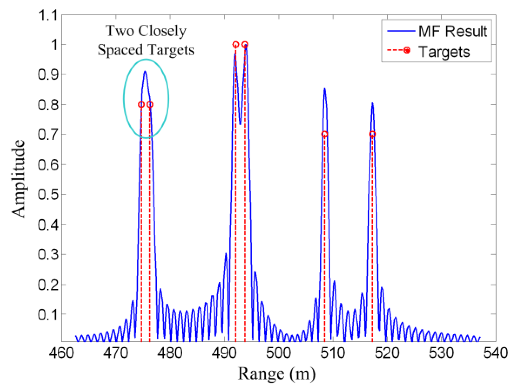
Figure 2 shows an example of the matched filtering method. Six point targets are set in the scene. It can be seen that the matched filtering result is the convolution of the targets and the autocorrelation of the system response. As a result, an idea point target is spread into a sinc waveform. Consequently, targets will interfere with each other, and two closely spaced targets may not be resolved in the matched filtering result.
Equation (7) is the original form of the matched filtering equation. In practice, in order to reduce the computational cost and make it more convenient for implementation, some transformations and approximations are usually adopted for Equation (7). Equation (7) can represent many widely used imaging algorithms, such as backprojection algorithms, range Doppler algorithms, chirp scaling algorithms, and ωK algorithms [1].

2.4. Regularization Method

Examining the LS formula (Equation (5)), it can be seen that it only relies on the observed data. In order to make the ill-posed inverse problem become well-posed, we can add an extra constraint to the LS formula [8,9,10]. This leads to the regularization method, which can be denoted as
g ^ = arg min g   { s - A g 2 2 + λ L ( g ) }
where λ is the regularization parameter and L ( g ) is the added penalty function. In order to make the solution of Equation (8) closer to the true value, L ( g ) should represent appropriate prior knowledge for the problem.
A typical choice of L ( g ) is
L ( g ) = g p p
where p denotes the l p -norm, i.e.,
g p = { ( i = 1 N | g i | p ) 1 / p p > 0 Number   of   nonzero   elements   in   g p = 0  
Then, Equation (8) can be rewritten as
g ^ = arg min g   { s - A g 2 2 + λ g p p }
The choice of p can control the result of the regularization method. If we want to enforce sparsity in the result, we should choose p in the range 0 p 1 [16,17]. For p = 1 , Equation (11) can be compared to the Lasso solution of the CS type methods [16]. Equation (11) can be solved by gradient search algorithms, such as the Newton iteration [22].

2.5. Bayesian Maximum a Posteriori Estimation

It should be noted that in Equation (11), the added constraint term λ g p p represents prior knowledge [17,23]. Another prior knowledge-based estimation method is Bayes theory. The main idea behind the Bayesian estimation framework is to account explicitly for the errors, and also for incomplete prior knowledge. Assuming that the noise n in Equation (3) is white and Gaussian, we have
p ( n ) exp { 1 2 σ 2 n 2 2 }
where σ 2 is the noise variance. Then we obtain the expression of likelihood
p ( s | g ) exp { 1 2 σ 2 s g 2 2 }
We assume that the scene has a prior probability density function, as
p ( g ) exp { α g p p }
If 0 p 1 , the magnitude of the scene is more likely to concentrate around zero, which implies that the scene is sparse. For a review on sparsity enforcing priors for the Bayesian estimation approach, the reader can refer to [6].
Using the prior probability density of g shown in (14), and according to the Bayes rule, we obtain
p ( g | s ) = p ( s | g ) p ( g ) p ( s ) 1 p ( s ) exp { 1 2 σ 2 s g 2 2 α g p p }
Then the MAP estimate can be obtained easily as
g ^ = arg max g p ( g | s ) = arg min g   s g 2 2 + 2 σ 2 α g p p
Comparing Equations (11) and (16), it can be seen that when λ = 2 σ 2 α , these two equations are equivalent, i.e., the regularization method is equivalent to Bayesian MAP estimation.

2.6. Compressed Sensing Method

For the observation model shown in Equation (3), if the scene (i.e., g ) is sparse, according to CS theory, it can be stably reconstructed using reduced data samples. The reconstruction method can be written as [16,17]
g ^ = arg min g   g 0   s . t .   s - A g 2 2 < ε
where s.t. means subject to and ε denotes the allowed data error in the reconstruction process.
Equation (17) is NP-hard and computationally difficult to solve [17]. Matching pursuit is an approximate method for obtaining an l 0 sparse solution. In CS theory, a more tractable approach is taking the l 1 -norm instead of the l 0 -norm, which is called the l 1 relaxation:
g ^ = arg min g   g 1   s . t .   s - A g 2 2 < ε
If g is sparse and A satisfies some specific conditions, Equations (18) and (17) will have the same solution, and this solution is the exact or approximate recovery of g [16,17]. Equation (18) can be solved using convex programming, which is more tractable than the original l 0 -norm minimum problem. Unlike the matched filtering method, CS method does not have an exact or pre-defined resolution, since it is a non-linear method. Generally, the resolution capability of the CS method is much better than the matched filtering method if the targets are sparse.
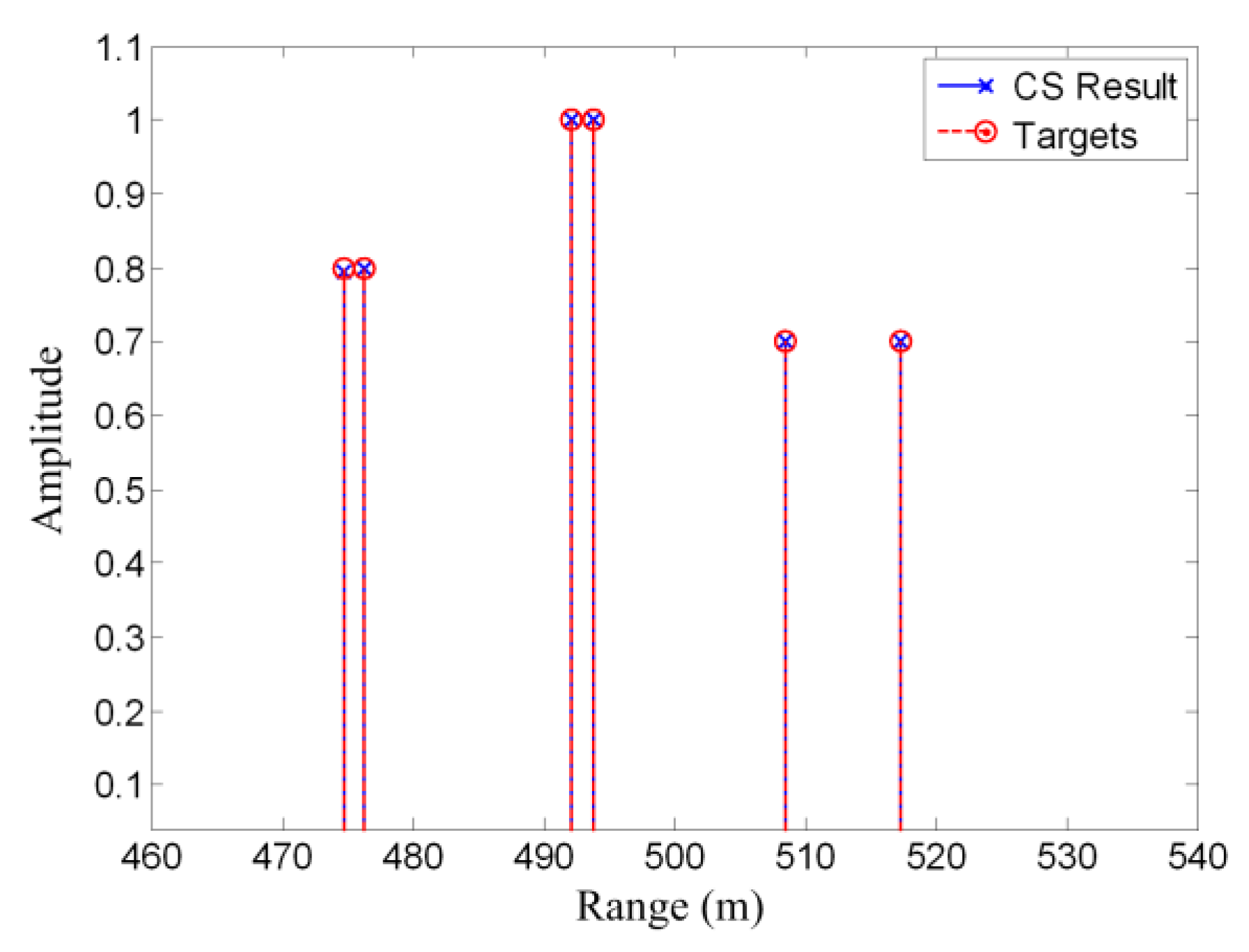
Figure 3 shows an example of compressed sensing. The simulated scene is the same as the matched filtering example shown in Figure 2. Only 1/20 signal samples are used for the CS reconstruction. It can be seen that the two closely spaced targets are well resolved. This implies that the CS method can obtain better results using less data than the matched filtering method. The reason is that prior information concerning signal sparsity is utilized in the CS model.
Equation (18) is a constrained optimization problem. According to the Lagrange theory, it can be transformed into an unconstrained optimization problem, which will have the same form as Equation (11). For appropriate choices of λ and p = 1 , Equations (11) and (18) will be equivalent [16,17]. This implies that CS is a special case of the regularization method.

2.7. Summary of Radar Imaging Methods

The above subsections introduced the LS estimator, matched filtering, regularization methods, Bayesian MAP estimation, and the CS method. In this subsection, we will summarize these methods and analyze their connections.
Table 1 lists the main characteristics and describes some connections between these imaging methods. The LS estimation only relies on the observed data, and cannot solve the ill-posed radar imaging problem efficiently. The matched filtering method can be viewed as using an approximation to avoid the ill-posed term in the LS solution. The regularization method, Bayesian MAP estimation, and the CS method exploit prior knowledge concerning the targets in addition to the observed data, and they are equivalent in some cases.
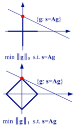
Table 1 also shows the equivalent geometric illustration for each method in 2 . The observation equation can only confine the solution to a hyperplane (which becomes a line in 2 ), but cannot reliably produce a certain solution [17,23]. The other methods aim at obtaining a stable solution close to the true value, using some modifications that represent prior knowledge concerning the targets.
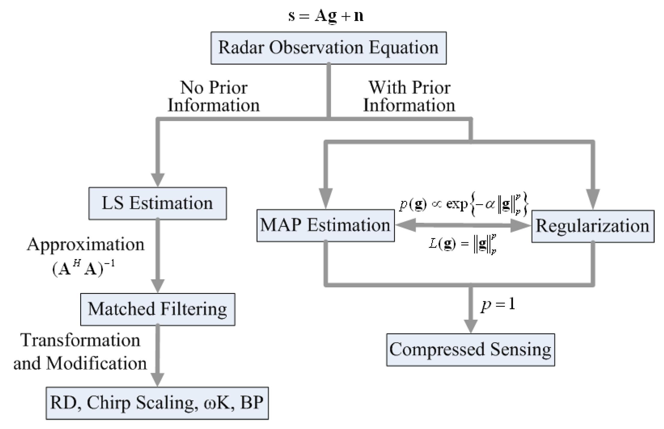
Figure 4 shows the block diagram and the relationship of the radar imaging methods. All of the radar imaging methods can be divided into two branches. The first branch does not use the prior information of the targets or scene, and it leads to the linear imaging methods; the most typical and widely used one in this branch is matched filtering. Another branch uses the prior information of the targets or scene. This leads to the non-linear methods. The most recently developed methods, including regularization methods, Bayesian methods, and CS methods belong to this branch.

3. Challenges and Advances in Compressed Sensing-Based Radar Imaging

The use of regularization methods in radar imaging goes back at least to the year 2000 [21,24]. Since the CS theory was proposed in 2006, it has been explored for a wide range of radar [25,26,27,28,29,30,31,32,33] and radar imaging applications [4,34,35,36,37,38], including synthetic aperture radar (SAR) [39,40,41,42], inverse SAR (ISAR) [43,44,45], tomographic SAR [46,47,48,49,50,51], three-dimensional (3D) SAR [52,53,54], SAR ground moving target indication (SAR/GMTI) [55,56,57,58,59,60,61], ground penetrating radar (GPR) [62,63,64], and through-the-wall radar (TWR) [65,66,67]. In this paper, we will focus on two-dimensional (2D) imaging radar systems, i.e., SAR, GPR, and TWR.
After several years of development, although many interesting ideas have been presented in this area, there still exist a number of challenges, both in theory and practice [68]. The state of the art in this area has not yet reached the stage of practical application. We will present some challenges as well as recent advances in this part of the paper.

3.1. Sampling Scheme

CS usually involves random under-sampling [16,17]. A widely used waveform in traditional radar imaging is the linear frequency modulated (LFM) waveform. If we adopt the LFM waveform in CS-based radar imaging, a random sampling analog to digital (A/D) converter is needed, which is not easily realized in practice. This will require extra hardware components, which means that LFM waveforms are not ideally suited for CS.
Recently, many researchers have found that the stepped frequency waveform is much more suitable for CS than the LFM waveform [35,62,63,66,69]. Sparse and discrete frequencies are more convenient for hardware implementation. For a CS-based radar imaging system, a stepped frequency waveform may be the preferred choice. In practical application, a set of adjustable pseudorandom numbers can be generated to select the frequency points in the stepped frequencies. In this way, randomly generated frequencies, i.e., random and sparse measurement, can be realized, and the CS-based imaging model can be implemented.
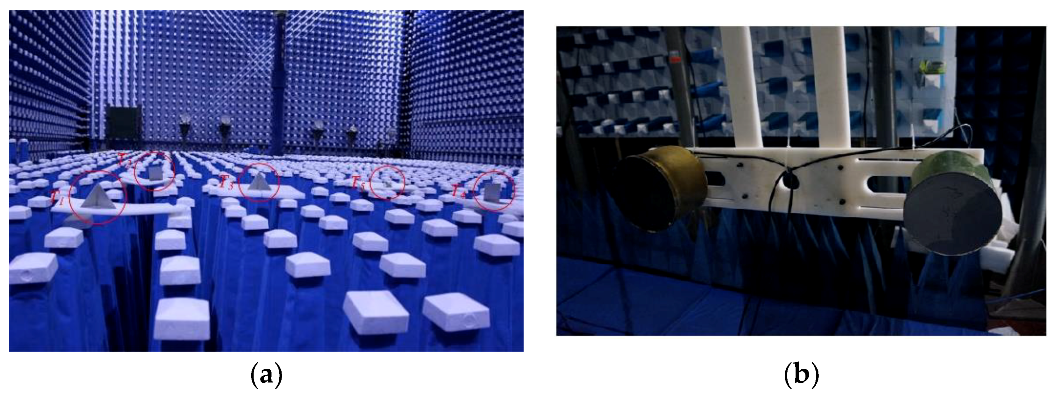
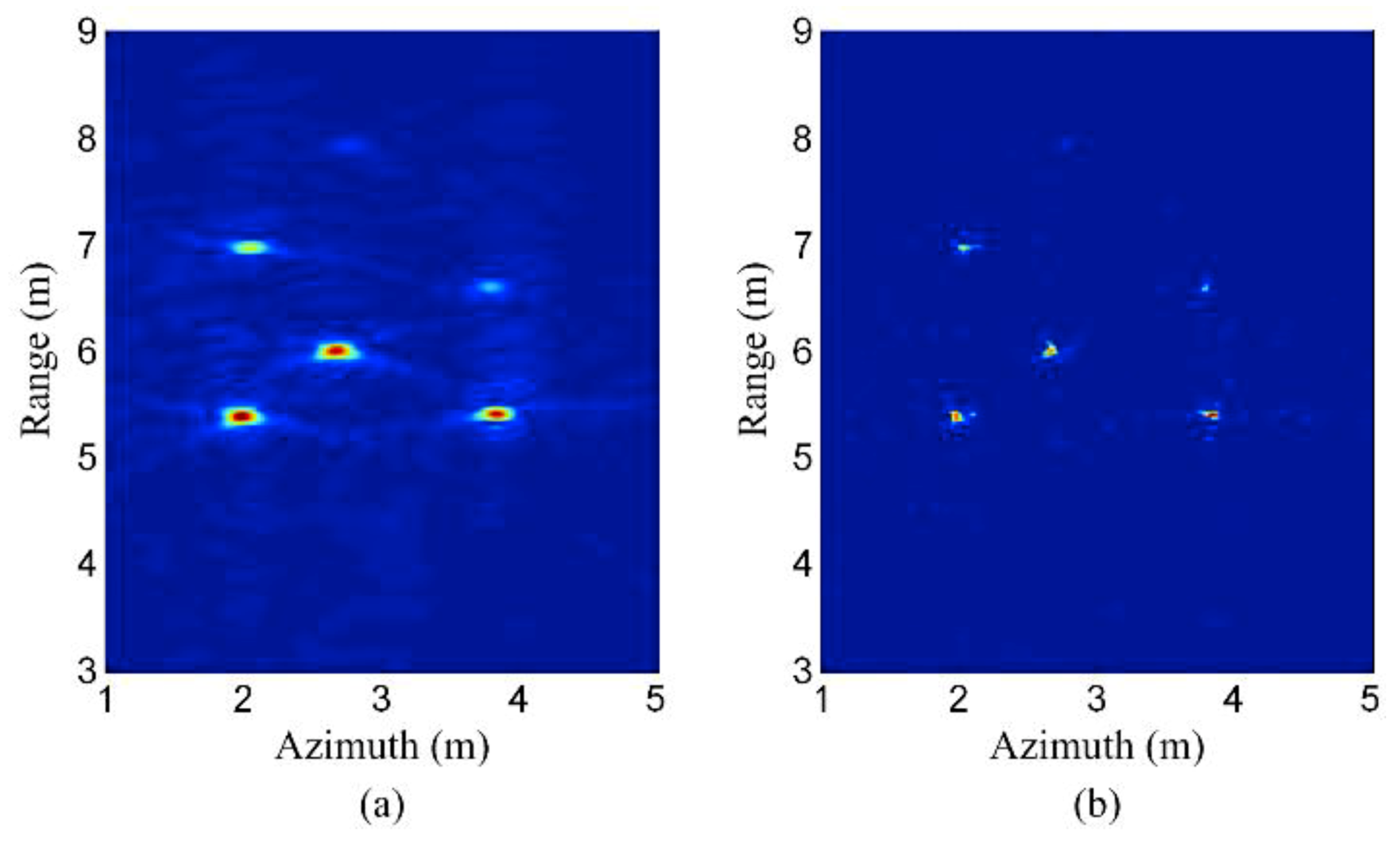
Figure 5 and Figure 6 show an example for CS-based stepped frequency radar imaging. The main equipment in the experimental system is a vector network analyzer (VNA). The experiment is carried out in a non-reflective microwave chamber. Five targets in the scene are shown in Figure 5. Figure 6a shows the backprojection result, using the fully sampled data (81 azimuth measurements × 2001 frequencies). Figure 6b shows the CS reconstruction result using under-sampled data (27 azimuth measurements × 128 frequencies). Considering the aspects of resolution and sidelobe levels, the CS reconstruction result is even better than the backprojection result, although it uses less sampled data. The reason is that prior information concerning signal sparsity is used in the CS model, while the backprojection method uses no prior information.

3.2. Computational Complexity

In the regularization or CS model for a 2D radar imaging system, the 2D observed data and the 2D scene grid are both stacked into column vectors. This will lead to a huge size measurement matrix. For example, the original fully sampled data are 2048 × 2540 points (azimuth × range); if a 512 × 512 pixel image is reconstructed from a reduced sampling data consist of 256 × 256 points. Then the size of the matrix A is 65,536 × 262,144. Since regularization or CS reconstruction is a non-linear process, such a large measurement matrix will result in a huge computational burden for image reconstruction. In addition, the total memory to access the measurement matrix is 128 gigabytes (assuming float point and complex numbers are used). This is a too much memory space for normal desktop computers. Considering that data size is usually larger than the above example in practice, it is difficult for conventional methods to reconstruct a moderate-size scene by using normal computers.
A common idea for reducing computational complexity and memory occupancy is to split big data into sets of small data [70]. Based on this thought, a segmented reconstruction method for CS based SAR imaging has been proposed [71]. In this method, the whole scene is split into a set of small subscenes. Since the computational complexity is non-linear to the data size, the reconstruction time can be reduced significantly. The sensing matrices for the method proposed in [71] are much smaller than those for the conventional method. Therefore, the method also needs much less memory. Due to the short reconstruction time and lower memory requirement of the method proposed in [71], reconstructing a moderate-size scene in a short time is no longer a difficult task. The processing steps of the segmented reconstruction method are shown in Figure 7.
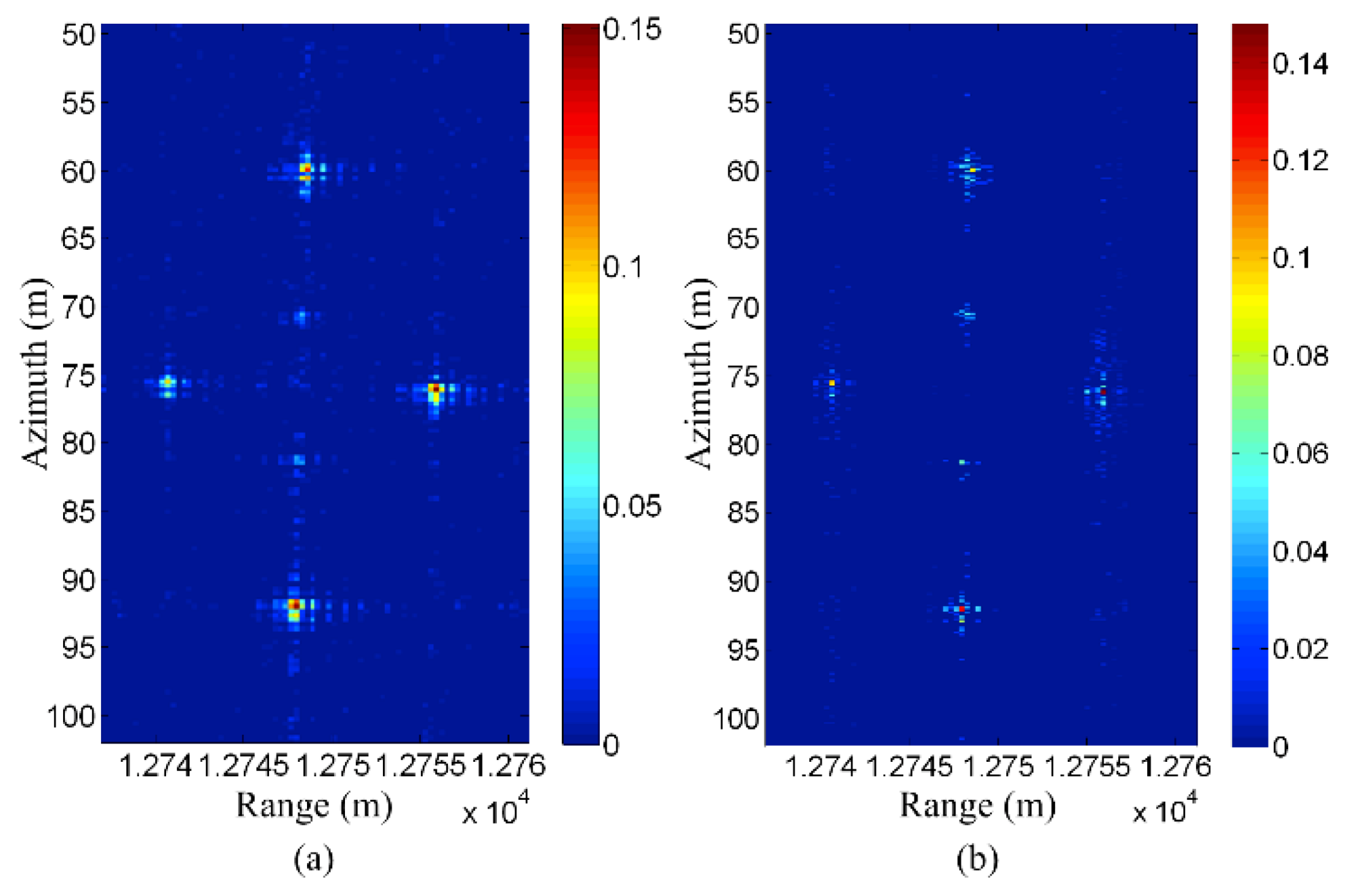
Figure 8 and Figure 9 show an example of the segmented reconstruction method [71]. Figure 8 shows the experimental scene of an airborne SAR system, which contains six trihedral reflectors. Figure 9a shows the conventional CS reconstruction result, where the reconstruction time is 44,032 s (12 h 14 min). The whole scene is split into five segments, and Figure 9b shows the segmented reconstruction result, where the reconstruction time is now reduced to 1498 s (25 min). It can be seen that, using the segmented reconstruction method, the reconstruction time is significantly reduced, while the reconstruction precision is nearly the same.

3.3. Sparsity and Sparse Representation

Sparsity of the scene is an essential requirement for sparse regularization or CS methods. For an SAR scene, an extended scene is usually not sparse in itself (not sparse in the canonical basis), except for the case of a few dominant scatterers in a low reflective background [35]. Therefore, a sparse representation is needed to use a sparsity-driven method.
CS-based optical imaging has successfully used sparse representations [72]. However, radar imaging involves complex-valued quantities; the raw data and the imaging result are both complex-valued. Since the phase of the scene are potentially random, it is very difficult to find a transform basis to sparsify a complex-valued and extended scene [73,74].
Structured dictionaries and dictionary learning ideas are proposed in [75] and [76], respectively. An alternative approach is to handle the magnitude and phase separately [41]. Although the phase of the scene is potentially random, the magnitude of the scene usually has better sparse characteristics. However, this approach has a much higher computational complexity than standard CS reconstruction. Another method investigates physical scattering behavior [4,77]. For example, a car can be represented as the superposition of responses from plate and dihedral shapes.
Figure 10 shows a simulation example for an extended and complex-valued scene. There are two extended objects in the scene, one of which has a round shape while the other has a rectangular shape. Both the two objects have random phases associated with them. It can be seen that the DCT (Discrete Cosine Transform) results of the magnitude are sparse.
Figure 11a shows the result of matched filtering. Since the random phase leads to speckle, it can be seen that although the scene has a smooth shape, the matched filtering result has obvious fluctuation. Figure 11b shows the result of conventional CS reconstruction without sparse representation. The reconstruction algorithm is SPGL1 [78]. Since the scene is not sparse in the canonical basis, the reconstruction is not accurate. Figure 11c shows the result of the method using a magnitude sparse representation [41]; it can be seen that the reconstruction result is much better than Figure 11a,b. Figure 11d shows the result of the method using the improved magnitude sparse representation method proposed in [79]. In the proposed method, besides the sparsity, the real-valued information of the magnitude and the coefficient distribution of the sparse representation are also utilized. It can be seen that both the shape and speckle are further improved.
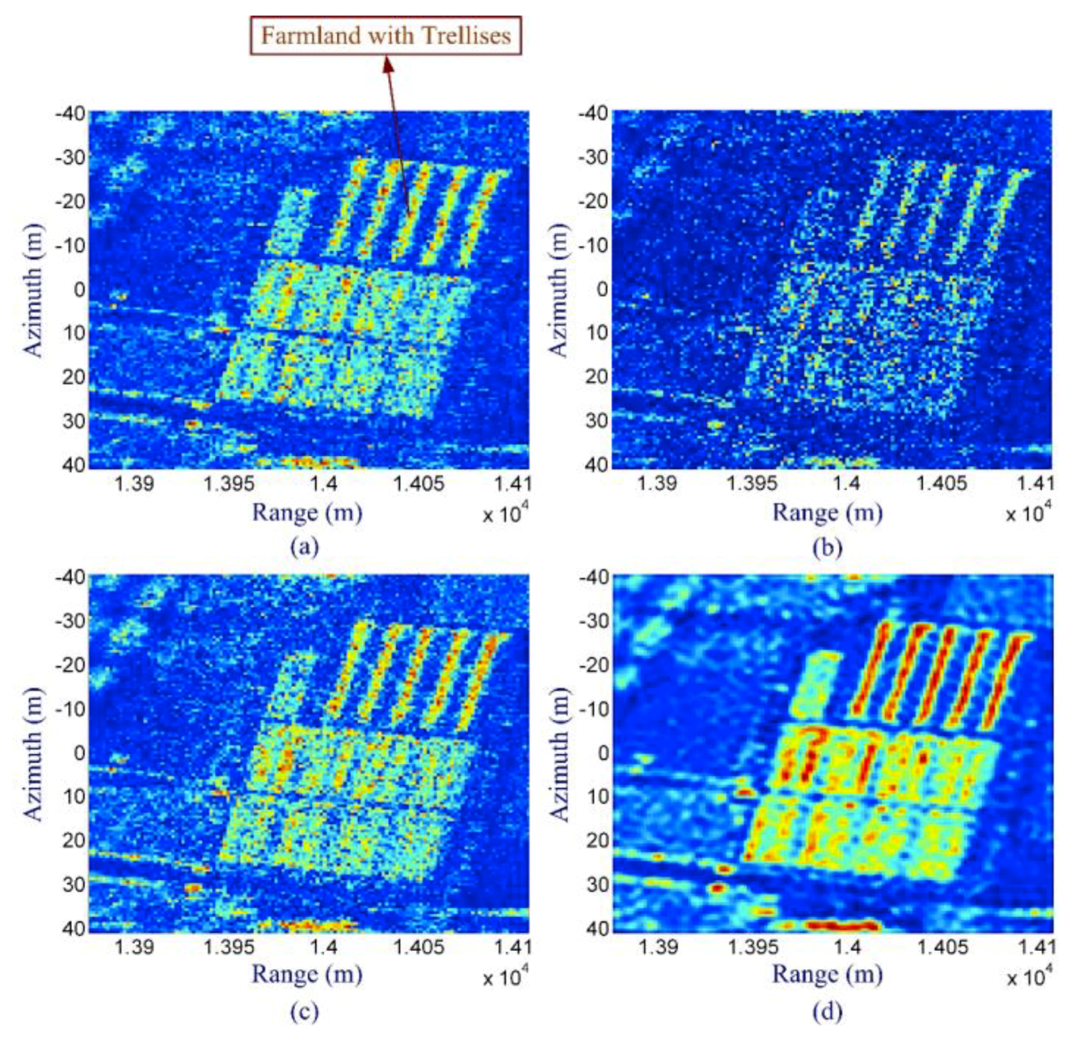
Figure 12 shows the real data results. The raw data is acquired by an airborne SAR system. Figure 12 contains a scene of farmland with trellises. The reflectivity from the trellises is very strong. From the real data result, it can be seen that CS with the improved magnitude sparse representation method can produce an image with less speckle and clearer edges of different regions than the previous methods.

3.4. Influence of Clutter

Another practical case is when the targets of interest are sparse, but there also exists clutter in the scene. Clutter arises from reflections within the scene, so the image may no longer be sparse if significant clutter returns are present. Typical examples include GPR and TWR imaging. The interesting targets, such as landmines and humans, are usually sparse, but they are often buried in the ground surface clutter and wall clutter.
Some methods have been proposed to remove the ground surface clutter and wall clutter for downward-looking GPR and TWR [64,65]. These methods are effective in cases when the clutter is concentrated in a fixed range cell or limited to several range cells.
Another scenario is TWR/SAR imaging of moving targets. A sparsity-driven change detection method is proposed in [67]. The stationary targets and clutter are removed via change detection, and then CS reconstruction is applied to the resulting sparse scene. In [55], a SAR/GMTI method using distributed CS is proposed, which can cope with the non-sparse stationary clutter.
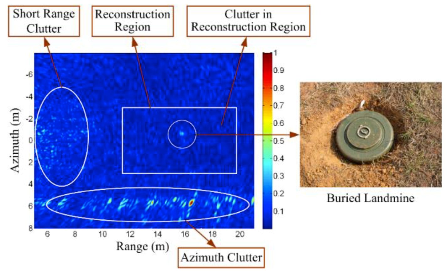
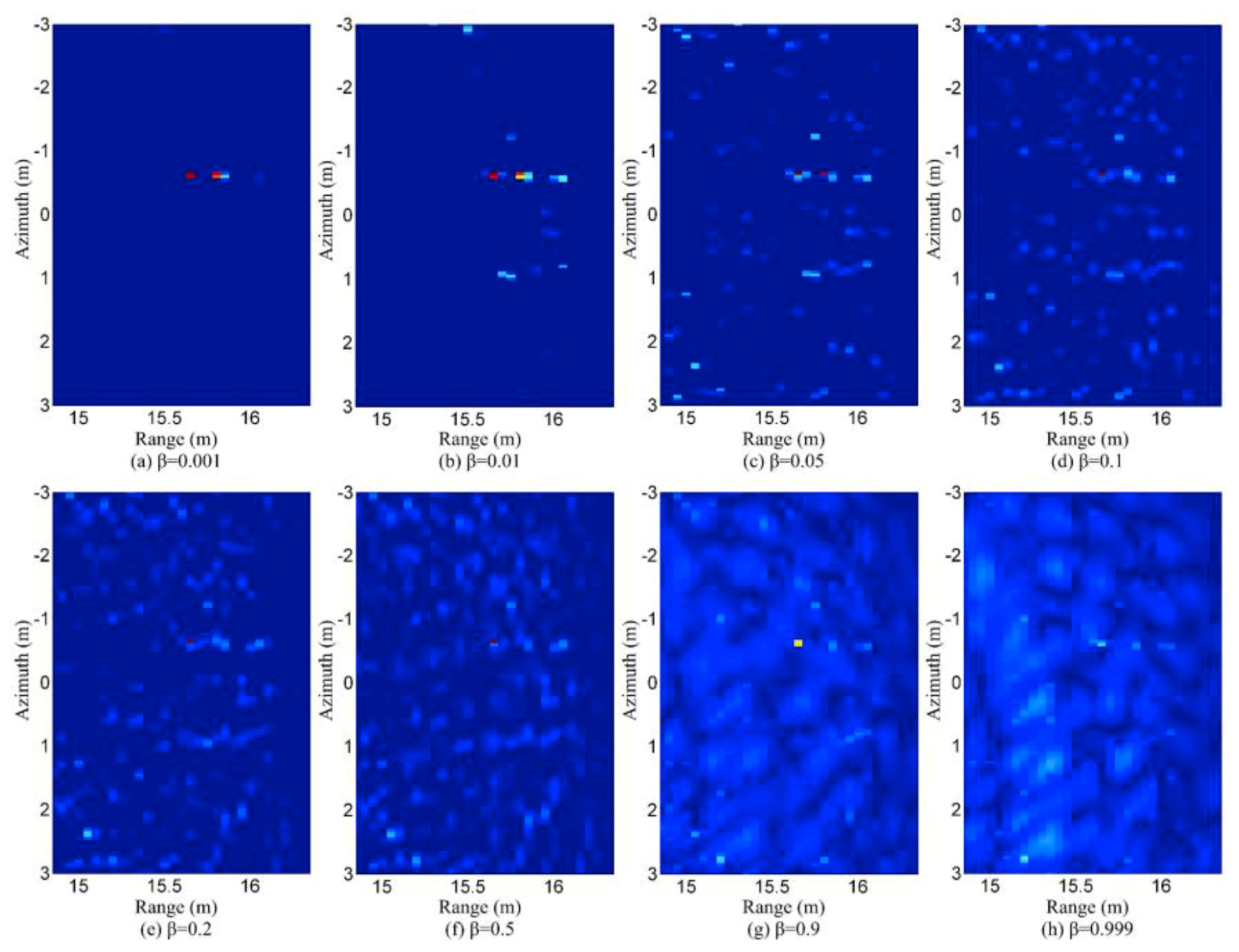
A more difficult case is when both the targets and clutter are stationary, and the clutter is distributed over the whole scene. Forward-looking GPR may fall into this category. Figure 13 shows a real data example for this case. In such a scenario, shrubs and rocks above the ground surface may cause strong azimuth clutter. Short range clutter is usually also strong, due to the large grazing angle and short range. Besides the strong clutter far away from the target (landmine), there is also ground surface clutter around the target. In [68], an idea is proposed to build a model in which the clutter is also taken into account as a norm in the objective function. In [80], the forward-looking clutter is suppressed in two steps. In the first step, the strong clutter outside of the reconstruction region is suppressed first. In the second step, the clutter in the reconstruction region is suppressed by selecting a proper β , which represents the ratio of the non-zeros area in the reconstructed scene. The reconstruction results are shown in Figure 14.

3.5. Model Error Compensation

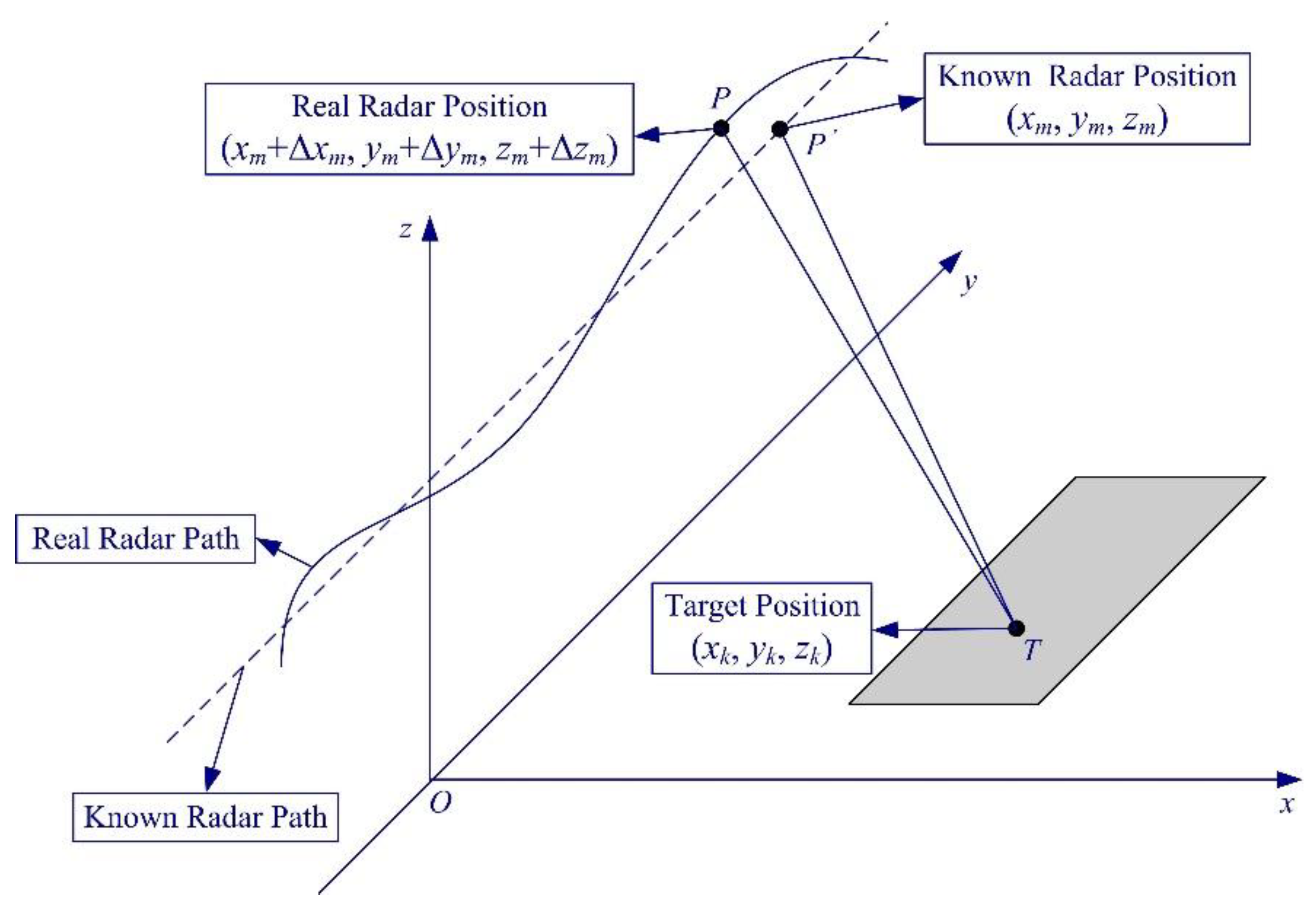
In the regularization or CS methods, we usually assume that the model is exact. However, in practice, the model may also contain errors. For example, imperfect knowledge of the observation position will lead to errors in the measurement matrix. This effect resembles motion errors that arise in traditional airborne SAR imaging. Figure 15 shows the geometry of the observation position errors or motion errors in SAR.
Several methods have been proposed to deal with model errors in CS-based or sparsity-driven radar imaging. A phase error correction method for sparsity-driven SAR imaging is proposed in [81]. An autofocus method for compressively sampled SAR is proposed in [82]. This method can correct phase errors in the reconstruction process. Both the methods proposed in [81,82] deal with phase errors in the observed data, or approximately treat the observation position-induced model errors as phase errors in the observed data. In [83], the platform position errors are investigated and compensated. That method considers the azimuth offset errors and also uses some approximations.
In [84], a model error compensation method is proposed. An iterative algorithm cycles through steps of target reconstruction, and observation position error estimation and compensation are used. This method can estimate the observation position error exactly, while only relying on the observed data.
Figure 16 shows a real data result using the method proposed in [84]. The data set used in this figure is the same as that used for Figure 9. In the data acquisition process, the airplane is expected to fly along a straight line. However, due to the air current’s influence, the trajectory of the airplane may slightly deviate from the expected one. As a result, the observation position data inevitably contain some errors.
Figure 16a shows the original CS reconstruction result. Since the observation position errors are not compensated, it can be seen that the targets are somewhat defocused. Figure 16b shows the corresponding CS reconstruction result with compensation for observation position error. It can be seen that the focusing quality is improved using the method proposed in [84]. The peak of the targets has an increase of about 20%, and the sidelobes are also significantly reduced.

4. Conclusions

In radar imaging area, there are many relevant techniques and methods, such as matched filtering, the range Doppler algorithm, the chirp scaling algorithm, the ωK algorithm, regularized methods, and CS methods. These techniques and methods are quite different in their forms. This paper tries to understand these techniques and methods in a unified mathematical framework.
Based on theoretical analysis, it can be seen that sparsity-driven regularization or CS-based radar imaging methods have potentially significant advantages. However, although many interesting ideas have been presented, very few of them have been verified with real data. There are still many unsolved or open problems in this area. In the issues discussed in this paper, the sampling scheme, fast reconstruction strategy, and model error problems are basically solved. However, issues concerning the sparsity or sparse representation of a complex and extended scene are still not completely solved. Strong clutter may break the sparsity of a scene, while sparse representation methods for an extended scene are currently not perfect. The state of the art in these areas has not yet reached the stage of practical application, and further investigations are needed in the future.

Funding

This work was supported in part by the National Natural Science Foundation of China under Grant 61401474, and in part by the Hunan Provincial Natural Science Foundation under Grant 2016JJ3025.

Conflicts of Interest

The authors declare no conflict of interest.

References

  1. Cumming, I.; Wong, F. Digital Processing of Synthetic Aperture Radar Data: Algorithms and Implementation; Artech House: Boston, MA, USA, 2005. [Google Scholar]
  2. Moreira, A.; Prats-Iraola, P.; Younis, M.; Krieger, G.; Hajnsek, I.; Papathanassiou, K.P. A tutorial on synthetic aperture radar. IEEE Geosci. Remote Sens. Mag. 2013, 1, 6–43. [Google Scholar] [CrossRef] [Green Version]
  3. Mensa, D.L. High Resolution Radar Imaging; Artech House: Norwood, MA, USA, 1981. [Google Scholar]
  4. Potter, L.C.; Ertin, E.; Parker, J.T.; Çetin, M. Sparsity and compressed sensing in radar imaging. Proc. IEEE 2010, 98, 1006–1020. [Google Scholar] [CrossRef]
  5. Mohammad-Djafari, A. Inverse Problems in Vision and 3D Tomography; ISTE: London, UK; John Wiley and Sons: New York, NY, USA, 2010. [Google Scholar]
  6. Mohammad-Djafari, A. Bayesian approach with prior models which enforce sparsity in signal and image processing. EURASIP J. Adv. Signal Process. 2012, 2012, 52. [Google Scholar] [CrossRef] [Green Version]
  7. Mohammad-Djafari, A.; Daout, F.; Fargette, P. Fusion and inversion of SAR data to obtain a superresolution image. In Proceedings of the IEEE International Conference on Image Processing (ICIP), Cario, Egypt, 7–10 November 2009; pp. 569–572. [Google Scholar]
  8. Groetsch, C.W. The Theory of Tikhonov Regularization for Fredholm Equations of the First Kind; Pitman Publishing Limited: London, UK, 1984. [Google Scholar]
  9. Tikhonov, A.N.; Arsenin, V.Y. Solutions of Ill-Posed Problems; Wiley: New York, NY, USA, 1977. [Google Scholar]
  10. Miller, K. Least squares methods for ill-posed problems with a prescribed bound. SIAM J. Math. Anal. 1970, 1, 52–57. [Google Scholar] [CrossRef]
  11. Blacknell, D.; Quegan, S. SAR super-resolution with a stochastic point spread function. In Proceedings of the IEE Colloquium on Synthetic Aperture Radar, London, UK, 29 November 1989. [Google Scholar]
  12. Pryde, G.C.; Delves, L.M.; Luttrell, S.P. Transputer based super resolution of SAR images: Two approaches to a parallel solution. In Proceedings of the IEE Colloquium on Transputers for Image Processing Applications, London, UK, 13 February 1989. [Google Scholar]
  13. Kay, S.M. Fundamentals of Statistical Signal Processing; Prentice Hall PTR: Upper Saddle River, NJ, USA, 1993. [Google Scholar]
  14. Bouman, C.; Sauer, K. A generalized Gaussian image model for edge-preserving MAP estimation. IEEE Trans. Image Process. 1993, 2, 296–310. [Google Scholar] [CrossRef] [PubMed]
  15. Chang, L.T.; Gupta, I.J.; Burnside, W.D.; Chang, C.T. A data compression technique for scattered fields from complex targets. IEEE Trans. Antennas Propag. 1997, 45, 1245–1251. [Google Scholar] [CrossRef]
  16. Candès, E.; Wakin, M.B. An introduction to compressive sampling. IEEE Signal Process. Mag. 2008, 25, 21–30. [Google Scholar] [CrossRef]
  17. Baraniuk, R.G. Compressive sensing. IEEE Signal Process. Mag. 2007, 24, 118–121. [Google Scholar] [CrossRef]
  18. Jafarpour, S.; Weiyu, X.; Hassibi, B.; Calderbank, R. Efficient and robust compressed sensing using optimized expander graphs. IEEE Trans. Inf. Theory 2009, 55, 4299–4308. [Google Scholar] [CrossRef]
  19. Yuejie, C.; Scharf, L.L.; Pezeshki, A.; Calderbank, R. Sensitivity to basis mismatch in compressed sensing. IEEE Trans. Signal Process. 2011, 59, 2182–2195. [Google Scholar]
  20. Raginsky, M.; Jafarpour, S.; Harmany, Z.T.; Marcia, R.F.; Willett, R.M.; Calderbank, R. Performance bounds for expander-based compressed sensing in Poisson noise. IEEE Trans. Signal Process. 2011, 59, 4139–4153. [Google Scholar] [CrossRef]
  21. Logan, C.L. An Estimation-Theoretic Technique for Motion Compensated Synthetic-Aperture Array Imaging. Ph.D. Thesis, Massachusetts Institute of Technology, Cambridge, MA, USA, 2000. [Google Scholar]
  22. Browne, K.E.; Burkholder, R.J.; Volakis, J.L. Fast optimization of through-wall radar images via the method of Lagrange multipliers. IEEE Trans. Antennas Propag. 2013, 61, 320–328. [Google Scholar] [CrossRef]
  23. Romberg, J. Imaging via compressive sampling. IEEE Signal Process. Mag. 2008, 25, 14–20. [Google Scholar] [CrossRef]
  24. Çetin, M.; Karl, W.C. Feature-enhanced synthetic aperture radar image formation based on nonquadratic regularization. IEEE Trans. Antennas Propag. 2001, 10, 623–631. [Google Scholar]
  25. Kalogerias, D.; Sun, S.; Petropulu, A.P. Sparse sensing in colocated MIMO radar: A matrix completion approach. In Proceedings of the 2013 IEEE International Symposium on Signal Processing and Information Technology (ISSPIT), Athens, Greece, 12–15 December 2013; pp. 496–502. [Google Scholar]
  26. Yao, Y.; Petropulu, A.P.; Poor, H.V. Measurement matrix design for compressive sensing-based MIMO radar. IEEE Trans. Signal Process. 2011, 59, 5338–5352. [Google Scholar]
  27. Yao, Y.; Petropulu, A.P.; Poor, H.V. MIMO radar using compressive sampling. IEEE J. Sel. Top. Signal Process. 2010, 4, 146–163. [Google Scholar]
  28. Rossi, M.; Haimovich, A.M.; Eldar, Y.C. Spatial compressive sensing for MIMO radar. IEEE Trans. Signal Process. 2014, 62, 419–430. [Google Scholar] [CrossRef]
  29. Rossi, M.; Haimovich, A.M.; Eldar, Y.C. Global methods for compressive sensing in MIMO radar with distributed sensors. In Proceedings of the Forty Fifth Asilomar Conference on Signals, Systems and Computers (ASILOMAR), Pacific Grove, CA, USA, 6–9 November 2011; pp. 1506–1510. [Google Scholar]
  30. Rossi, M.; Haimovich, A.M.; Eldar, Y.C. Spatial compressive sensing in MIMO radar with random arrays. In Proceedings of the 46th Annual Conference on Information Sciences and Systems (CISS), Princeton, NJ, USA, 21–23 March 2012. [Google Scholar]
  31. Herman, M.; Strohmer, T. Compressed sensing radar. In Proceedings of the 2008 IEEE Radar Conference, Rome, Italy, 26–30 May 2008. [Google Scholar]
  32. Herman, M.; Strohmer, T. High-resolution radar via compressed sensing. IEEE Trans. Signal Process. 2009, 57, 2275–2284. [Google Scholar] [CrossRef]
  33. Herman, M.; Strohmer, T. General deviants: An analysis of perturbations in compressed sensing. IEEE J. Sel. Top. Signal Process. 2010, 4, 342–349. [Google Scholar] [CrossRef]
  34. Baraniuk, R.G.; Steeghs, P. Compressive radar imaging. In Proceedings of the 2007 IEEE Radar Conference, Boston, MA, USA, 17–20 April 2007; pp. 128–133. [Google Scholar]
  35. Ender, J.H.G. On compressive sensing applied to radar. Signal Process. 2010, 90, 1402–1414. [Google Scholar] [CrossRef]
  36. Çetin, M.; Stojanovic, I.; Önhon, N.Ö.; Varshney, K.; Samadi, S.; Karl, W.C.; Willsky, A. Sparsity-driven synthetic aperture radar imaging: Reconstruction, autofocusing, moving targets, and compressed sensing. IEEE Signal Process. Mag. 2014, 31, 27–40. [Google Scholar] [CrossRef]
  37. Zhang, B.; Hong, W.; Wu, Y. Sparse microwave imaging: Principles and applications. Sci. China Inf. Sci. 2012, 55, 1722–1754. [Google Scholar] [CrossRef] [Green Version]
  38. Bi, H.; Zhang, B.; Zhu, X.; Jiang, C.; Hong, W. Extended chirp scaling-baseband azimuth scaling-based azimuth-range decouple L1 regularization for TOPS SAR imaging via CAMP. IEEE Trans. Geosci. Remote Sens. 2017, 55, 3748–3763. [Google Scholar] [CrossRef]
  39. Patel, V.M.; Easley, G.R.; Healy, D.M., Jr.; Chellappa, R. Compressed synthetic aperture radar. IEEE J. Sel. Top. Signal Process. 2010, 4, 244–254. [Google Scholar] [CrossRef]
  40. Alonso, M.T.; López-Dekker, P.; Mallorquí, J.J. A novel strategy for radar imaging based on compressive sensing. IEEE Trans. Geosci. Remote Sens. 2010, 48, 4285–4295. [Google Scholar] [CrossRef]
  41. Samadi, S.; Çetin, M.; Masnadi-Shirazi, M.A. Sparse representation-based synthetic aperture radar imaging. IET Radar Sonar Navig. 2011, 5, 182–193. [Google Scholar] [CrossRef] [Green Version]
  42. Yang, L.; Zhou, J.; Hu, L.; Xiao, H. A Perturbation-Based Approach for Compressed Sensing Radar Imaging. IEEE Antennas Wirel. Propag. Lett. 2017, 16, 87–90. [Google Scholar] [CrossRef]
  43. Zhang, L.; Qiao, Z.; Xing, M.; Li, Y.; Bao, Z. High-Resolution ISAR imaging with sparse stepped-frequency waveforms. IEEE Trans. Geosci. Remote Sens. 2011, 49, 4630–4651. [Google Scholar] [CrossRef]
  44. Wang, H.; Quan, Y.; Xing, M.; Zhang, S. ISAR Imaging via sparse probing frequencies. IEEE Geosci. Remote Sens. Lett. 2011, 8, 451–455. [Google Scholar] [CrossRef]
  45. Du, X.; Duan, C.; Hu, W. Sparse representation based autofocusing technique for ISAR images. IEEE Trans. Geosci. Remote Sens. 2013, 51, 1826–1835. [Google Scholar] [CrossRef]
  46. Zhu, X.X.; Bamler, R. Tomographic SAR inversion by L1-norm regularization-the compressive sensing approach. IEEE Trans. Geosci. Remote Sens. 2010, 48, 3839–3846. [Google Scholar] [CrossRef]
  47. Zhu, X.X.; Bamler, R. Super-resolution power and robustness of compressive sensing for spectral estimation with application to spaceborne tomographic SAR. IEEE Trans. Geosci. Remote Sens. 2012, 50, 247–258. [Google Scholar] [CrossRef]
  48. Zhu, X.X.; Ge, N.; Shahzad, M. Joint Sparsity in SAR Tomography for Urban Mapping. IEEE J. Sel. Top. Signal Process. 2015, 9, 1498–1509. [Google Scholar] [CrossRef] [Green Version]
  49. Budillon, A.; Evangelista, A.; Schirinzi, G. Three-Dimensional SAR Focusing from Multipass Signals Using Compressive Sampling. IEEE Trans. Geosci. Remote Sens. 2011, 49, 488–499. [Google Scholar] [CrossRef]
  50. Xilong, S.; Anxi, Y.; Zhen, D.; Diannong, L. Three-dimensional SAR focusing via compressive sensing: The case study of angel stadium. IEEE Geosci. Remote Sens. Lett. 2012, 9, 759–763. [Google Scholar] [CrossRef]
  51. Aguilera, E.; Nannini, M.; Reigber, A. Multisignal compressed sensing for polarimetric SAR tomography. IEEE Geosci. Remote Sens. Lett. 2012, 9, 871–875. [Google Scholar] [CrossRef]
  52. Kajbaf, H. Compressed Sensing for 3D Microwave Imaging Systems. Ph.D. Thesis, Missouri University of Science and Technology, Rolla, MO, USA, 2012. [Google Scholar]
  53. Zhang, S.; Dong, G.; Kuang, G. Superresolution downward-looking linear array three-dimensional SAR imaging based on two-dimensional compressive sensing. IEEE J. Sel. Top. Appl. Earth Obs. Remote Sens. 2016, 9, 2184–2196. [Google Scholar] [CrossRef]
  54. Tian, H.; Li, D. Sparse flight array SAR downward-looking 3-D imaging based on compressed sensing. IEEE Geosci. Remote Sens. Lett. 2016, 13, 1395–1399. [Google Scholar] [CrossRef]
  55. Lin, Y.G.; Zhang, B.C.; Hong, W.; Wu, Y.R. Along-track interferometric SAR imaging based on distributed compressed sensing. Electron. Lett. 2010, 46, 858–860. [Google Scholar] [CrossRef]
  56. Prünte, L. Compressed sensing for joint ground imaging and target indication with airborne radar. In Proceedings of the 4th Workshop on Signal Processing with Adaptive Sparse Structured Representations, Edinburgh, UK, 27–30 June 2011. [Google Scholar]
  57. Wu, Q.; Xing, M.; Qiu, C.; Liu, B.; Bao, Z.; Yeo, T.S. Motion parameter estimation in the SAR system with low PRF sampling. IEEE Geosci. Remote Sens. Lett. 2010, 7, 450–454. [Google Scholar] [CrossRef]
  58. Stojanovic, I.; Karl, W.C. Imaging of moving targets with multi-static SAR using an overcomplete dictionary. IEEE J. Sel. Top. Signal Process. 2010, 4, 164–176. [Google Scholar] [CrossRef]
  59. Önhon, N.Ö.; Çetin, M. SAR moving target imaging in a sparsity-driven framework. In Proceedings of the SPIE Optics + Photonics Symposium, Wavelets and Sparsity XIV, San Diego, CA, USA, 21–25 August 2011; Volume 8138, pp. 1–9. [Google Scholar]
  60. Prünte, L. Detection performance of GMTI from SAR images with CS. In Proceedings of the 2014 European Conference on Synthetic Aperture Radar, Berlin, Germany, 3–5 June 2014. [Google Scholar]
  61. Prünte, L. Compressed sensing for removing moving target artifacts and reducing noise in SAR images. In Proceedings of the European Conference on Synthetic Aperture Radar, Hamburg, Germany, 6–9 June 2016. [Google Scholar]
  62. Suksmono, A.B.; Bharata, E.; Lestari, A.A.; Yarovoy, A.G.; Ligthart, L.P. Compressive stepped-frequency continuous-wave ground-penetrating radar. IEEE Geosci. Remote Sens. Lett. 2010, 7, 665–669. [Google Scholar] [CrossRef]
  63. Gurbuz, A.C.; McClellan, J.H.; Scott, W.R. A compressive sensing data acquisition and imaging method for stepped frequency GPRs. IEEE Trans. Signal Process. 2009, 57, 2640–2650. [Google Scholar] [CrossRef]
  64. Tuncer, M.A.C.; Gurbuz, A.C. Ground reflection removal in compressive sensing ground penetrating radars. IEEE Geosci. Remote Sens. Lett. 2012, 9, 23–27. [Google Scholar] [CrossRef]
  65. Lagunas, E.; Amin, M.G.; Ahmad, F.; Nájar, M. Joint wall mitigation and compressive sensing for indoor image reconstruction. IEEE Trans. Geosci. Remote Sens. 2013, 51, 891–906. [Google Scholar] [CrossRef]
  66. Amin, M.G. Through-the-Wall Radar Imaging; CRC Press: Boca Raton, FL, USA, 2010. [Google Scholar]
  67. Ahmad, F.; Amin, M.G. Through-the-wall human motion indication using sparsity-driven change detection. IEEE Trans. Geosci. Remote Sens. 2013, 51, 881–890. [Google Scholar] [CrossRef]
  68. Strohmer, T. Radar and compressive sensing—A perfect couple? In Proceedings of the Keynote Speak of 1st International Workshop on Compressed Sensing Applied to Radar (CoSeRa 2012), Bonn, Germany, 14–16 May 2012. [Google Scholar]
  69. Yang, J.; Thompson, J.; Huang, X.; Jin, T.; Zhou, Z. Random-frequency SAR imaging based on compressed sensing. IEEE Trans. Geosci. Remote Sens. 2013, 51, 983–994. [Google Scholar] [CrossRef]
  70. Qin, S.; Zhang, Y.D.; Wu, Q.; Amin, M. Large-scale sparse reconstruction through partitioned compressive sensing. In Proceedings of the International Conference on Digital Signal Processing, Hong Kong, China, 20–23 August 2014; pp. 837–840. [Google Scholar]
  71. Yang, J.; Thompson, J.; Huang, X.; Jin, T.; Zhou, Z. Segmented reconstruction for compressed sensing SAR imaging. IEEE Trans. Geosci. Remote Sens. 2013, 51, 4214–4225. [Google Scholar] [CrossRef]
  72. Duarte, M.F.; Davenport, M.A.; Takhar, D.; Laska, J.N.; Sun, T.; Kelly, K.F.; Baraniuk, R.G. Single-pixel imaging via compressive sampling. IEEE Signal Process. Mag. 2008, 25, 83–91. [Google Scholar] [CrossRef] [Green Version]
  73. Çetin, M.; Karl, W.C.; Willsky, A.S. Feature-preserving regularization method for complex-valued inverse problems with application to coherent imaging. Opt. Eng. 2006, 45, 017003. [Google Scholar]
  74. Çetin, M.; Önhon, N.Ö.; Samadi, S. Handling phase in sparse reconstruction for SAR: Imaging, autofocusing, and moving targets. In Proceedings of the EUSAR 2012—9th European Conference on Synthetic Aperture Radar, Nuremberg, Germany, 23–26 April 2012. [Google Scholar]
  75. Varshney, K.R.; Çetin, M.; Fisher, J.W., III; Willsky, A.S. Sparse representation in structured dictionaries with application to synthetic aperture radar. IEEE Trans. Signal Process. 2008, 56, 3548–3560. [Google Scholar] [CrossRef]
  76. Abolghasemi, V.; Gan, L. Dictionary learning for incomplete SAR data. In Proceedings of the CoSeRa 2012, Bonn, Germany, 14–16 May 2012. [Google Scholar]
  77. Halman, J.; Burkholder, R.J. Sparse expansions using physical and polynomial basis functions for compressed sensing of frequency domain EM scattering. IEEE Antennas Wirel. Propag. Lett. 2015, 14, 1048–1051. [Google Scholar] [CrossRef]
  78. Van Den Berg, E.; Friedlander, M.P. Probing the Pareto frontier for basis pursuit solutions. SIAM J. Sci. Comput. 2008, 31, 890–912. [Google Scholar] [CrossRef]
  79. Yang, J.; Jin, T.; Huang, X. Compressed sensing radar imaging with magnitude sparse representation. IEEE Access 2019, 7, 29722–29733. [Google Scholar] [CrossRef]
  80. Yang, J.; Jin, T.; Huang, X.; Thompson, J.; Zhou, Z. Sparse MIMO array forward-looking GPR imaging based on compressed sensing in clutter environment. IEEE Trans. Geosci. Remote Sens. 2014, 52, 4480–4494. [Google Scholar] [CrossRef]
  81. Önhon, N.Ö.; Çetin, M. A sparsity-driven approach for joint SAR imaging and phase error correction. IEEE Trans. Antennas Propag. 2012, 21, 2075–2088. [Google Scholar]
  82. Kelly, S.I.; Yaghoobi, M.; Davies, M.E. Auto-focus for compressively sampled SAR. In Proceedings of the CoSeRa 2012, Bonn, Germany, 14–16 May 2012. [Google Scholar]
  83. Wei, S.J.; Zhang, X.L.; Shi, J. An autofocus approach for model error correction in compressed sensing SAR imaging. In Proceedings of the IEEE International Geoscience and Remote Sensing Symposium (IGARSS 2012), Munich, Germany, 22–27 July 2012. [Google Scholar]
  84. Yang, J.; Huang, X.; Thompson, J.; Jin, T.; Zhou, Z. Compressed sensing radar imaging with compensation of observation position error. IEEE Trans. Geosci. Remote Sens. 2014, 52, 4608–4620. [Google Scholar] [CrossRef]
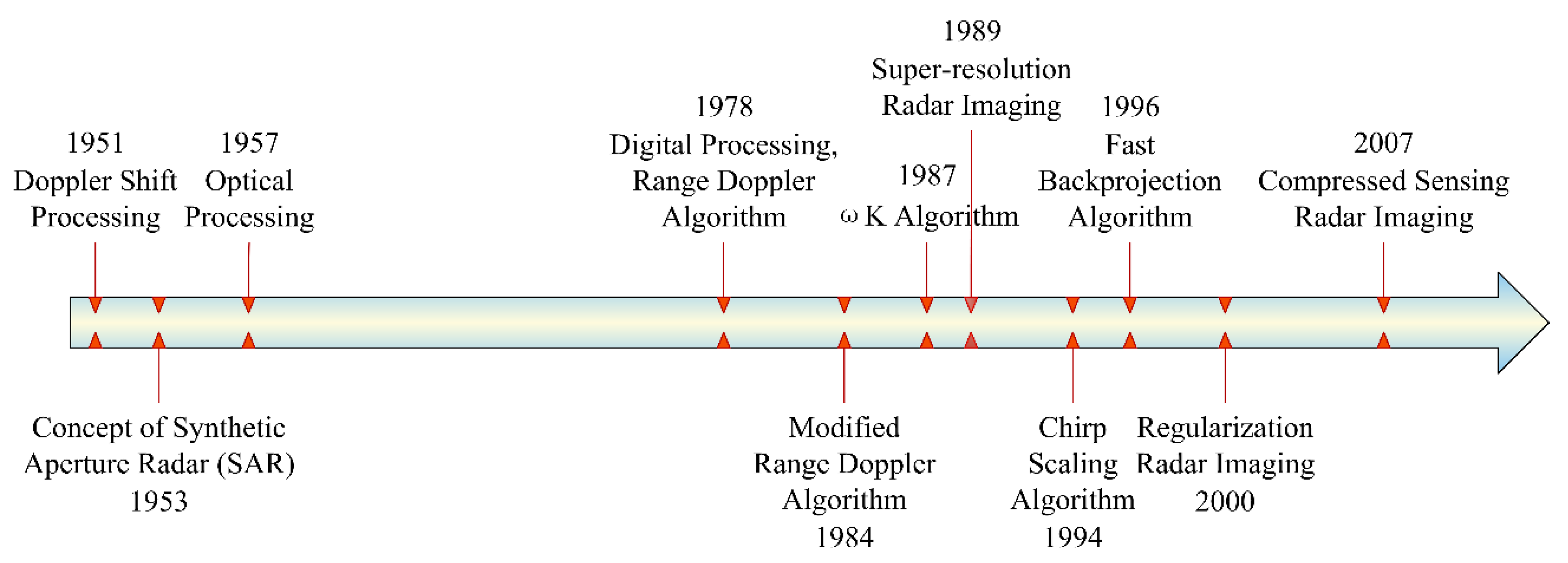
Figure 1. Developmental history of radar imaging methods.
Sensors 19 03100 g001
Figure 2. Matched filtering example. Two closely spaced targets cannot be resolved.
Sensors 19 03100 g002
Figure 3. Compressed sensing example; closely spaced targets are well resolved.
Sensors 19 03100 g003
Figure 4. Block diagram and relationship of the radar imaging methods.
Sensors 19 03100 g004
Figure 5. Experimental scene for CS-based stepped frequency radar imaging. (a) Five reflectors in the microwave chamber. (b) Transmitter and receiver antennas.
Sensors 19 03100 g005
Figure 6. (a) Backprojection result of full data (81 azimuth measurements × 2001 frequencies). (b) CS result of under-sampled data (27 azimuth measurements × 128 frequencies).
Sensors 19 03100 g006
Figure 7. Processing steps of the segmented reconstruction method for CS-based synthetic aperture radar (SAR) imaging (taken from [71]).
Sensors 19 03100 g007
Figure 8. Trihedral reflectors in the scene. Trihedral reflectors 1–4 are large, and trihedral reflectors 5 and 6 are small (taken from [71]).
Sensors 19 03100 g008
Figure 9. (a) Conventional CS reconstruction result (reconstruction time = 44,032 s). (b) Segmented reconstruction result (reconstruction time = 1498 s) (taken from [71]).
Sensors 19 03100 g009
Figure 10. (a) Magnitude of the scene, (b) phase of the scene, (c) DCT result of the magnitude (taken from [79]).
Sensors 19 03100 g010
Figure 11. Simulation results: (a) matched filtering result, (b) conventional CS reconstruction result without sparse representation, (c) result of the method with magnitude sparse representation, and (d) result of the method with improved magnitude sparse representation (taken from [79]).
Sensors 19 03100 g011
Figure 12. Real data reconstruction results (scene of farmland with trellises): (a) matched filtering result (full data), (b) conventional CS reconstruction result without sparse representation, (c) result of CS with magnitude sparse representation, and (d) result of CS with improved magnitude sparse representation (taken from [79]).
Sensors 19 03100 g012
Figure 13. Real data example for the clutter problem in forward-looking GPR (backprojection result using full-sampled data). Taken from [80].
Sensors 19 03100 g013
Figure 14. Reconstruction results in clutter environment with different parameters (taken from [80]).
Sensors 19 03100 g014
Figure 15. Geometry of the observation position errors in SAR. (Taken from [84]).
Sensors 19 03100 g015
Figure 16. Observation position error compensation for airborne SAR data. (a) Result without observation position error compensation. (b) Result with observation position error compensation (taken from [84]).
Sensors 19 03100 g016
Table 1. Characteristics and connections of radar imaging methods.
Radar   Observation   Model :   s = A g + n
s :   Observed   Data , A :   Measurement   Matrix , g :   Scene ,   n
Imaging MethodsMathematical ModelCharacteristicsEquivalent Geometric Illustration
Least Squares (LS) Estimation g ^ = arg min g   s - A g 2 2 g ^ = ( A H A ) 1 A H s , ( A H A ) 1 is usually ill-posed or nonexistent, cannot obtain a stable solution [9,13]. Sensors 19 03100 i001
Matched Filtering g ^ = A H s Avoids the ill-posed term in the LS solution, but the resolution is limited by the system bandwidth, and side-lobes will appear in the final image [4,21]. Sensors 19 03100 i002
Range Doppler, Chirp Scaling, ωK, etc.Approximations and transformations of A H s Approximations and transformations of the original matched filtering, in order to reduce the computational cost and make it more convenient to implement in practice [1]. Sensors 19 03100 i003
Regularization Method g ^ = arg min g   s - A g 2 2 + λ L ( g ) Add an extra constraint to the LS formula, so that the ill-posed inverse problem becomes well-posed. If the added constraint is chosen appropriately, the result will be better than that for matched filtering [8,9].Depends on the expression of L ( g ) .
Sparsity-Driven Regularization g ^ = arg min g   s - A g 2 2 + λ g p p
0 p 1
Choose L ( g ) as the l p -norm ( 0 p 1 ), in order to obtain sparse reconstruction result [6,23]. Sensors 19 03100 i004
Bayesian MAP Estimation p ( g ) exp { α g p p }
g ^ = arg min g   s - A g 2 2 + 2 σ 2 α g p p
For 2 σ 2 α = λ , the MAP estimation will be equivalent to the sparsity-driven regularization method [6,14]. Sensors 19 03100 i005
Compressed Sensing (CS) Method g ^ = arg min g   g 0   s . t .   s - A g 2 2 < ε
or
g ^ = arg min g   g 1   s . t .   s - A g 2 2 < ε
For an appropriate choice of λ , the CS method will be equivalent to the sparsity-driven regularization method [17,23]. Sensors 19 03100 i006