An Efficient Extended Targets Detection Framework Based on Sampling and Spatio-Temporal Detection

Abstract
1. Introduction
2. Models and Notations
2.1. Target Model
2.2. Noise Model
2.3. Measurement Model
2.4. Problem Statement
3. Proposed Methods
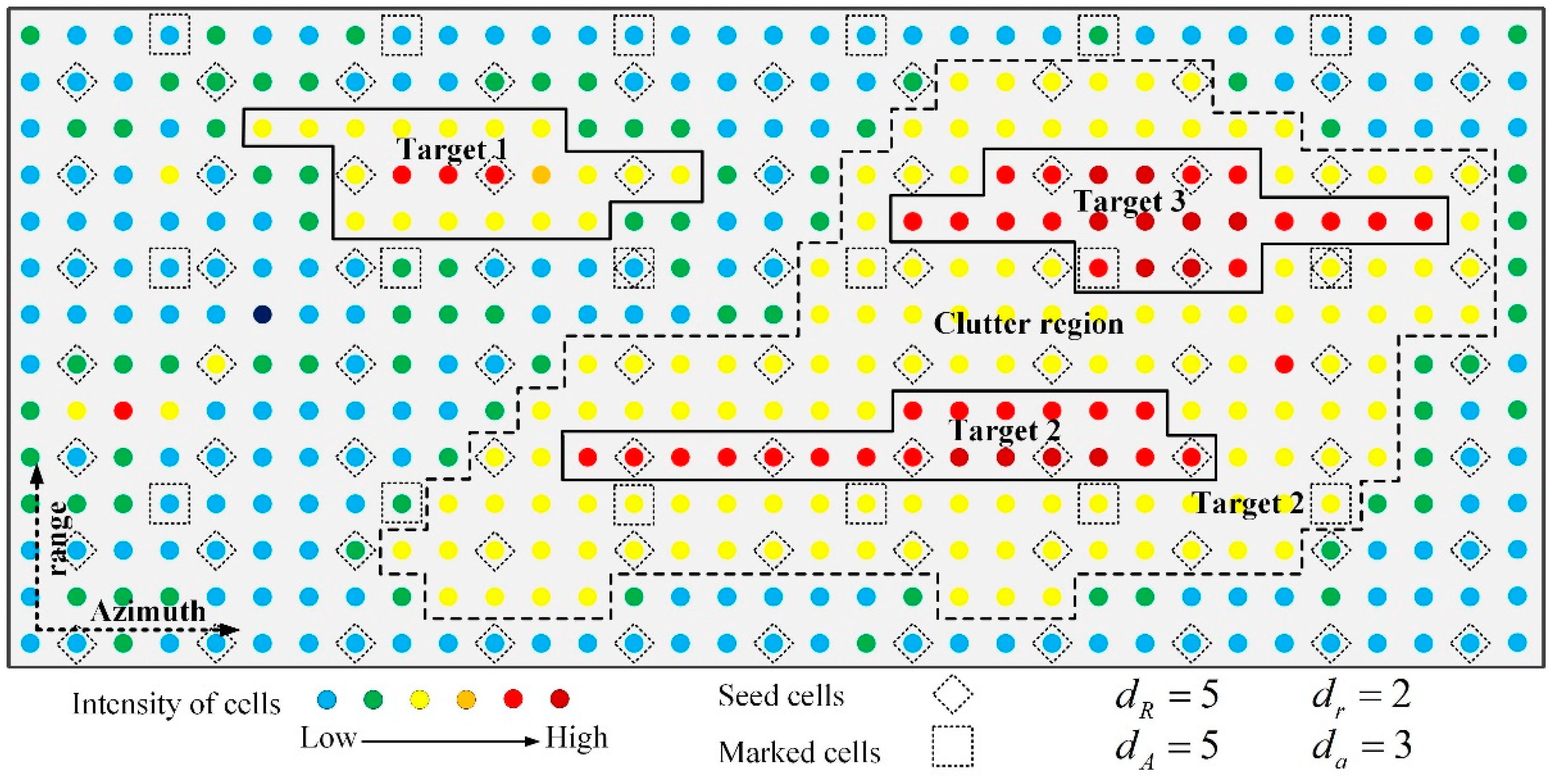
3.1. Sampling-Based Spatiotemporal Thresholding Method
3.2. The Proposed Detection Framework
4. Experiment and Results
4.1. Real Data
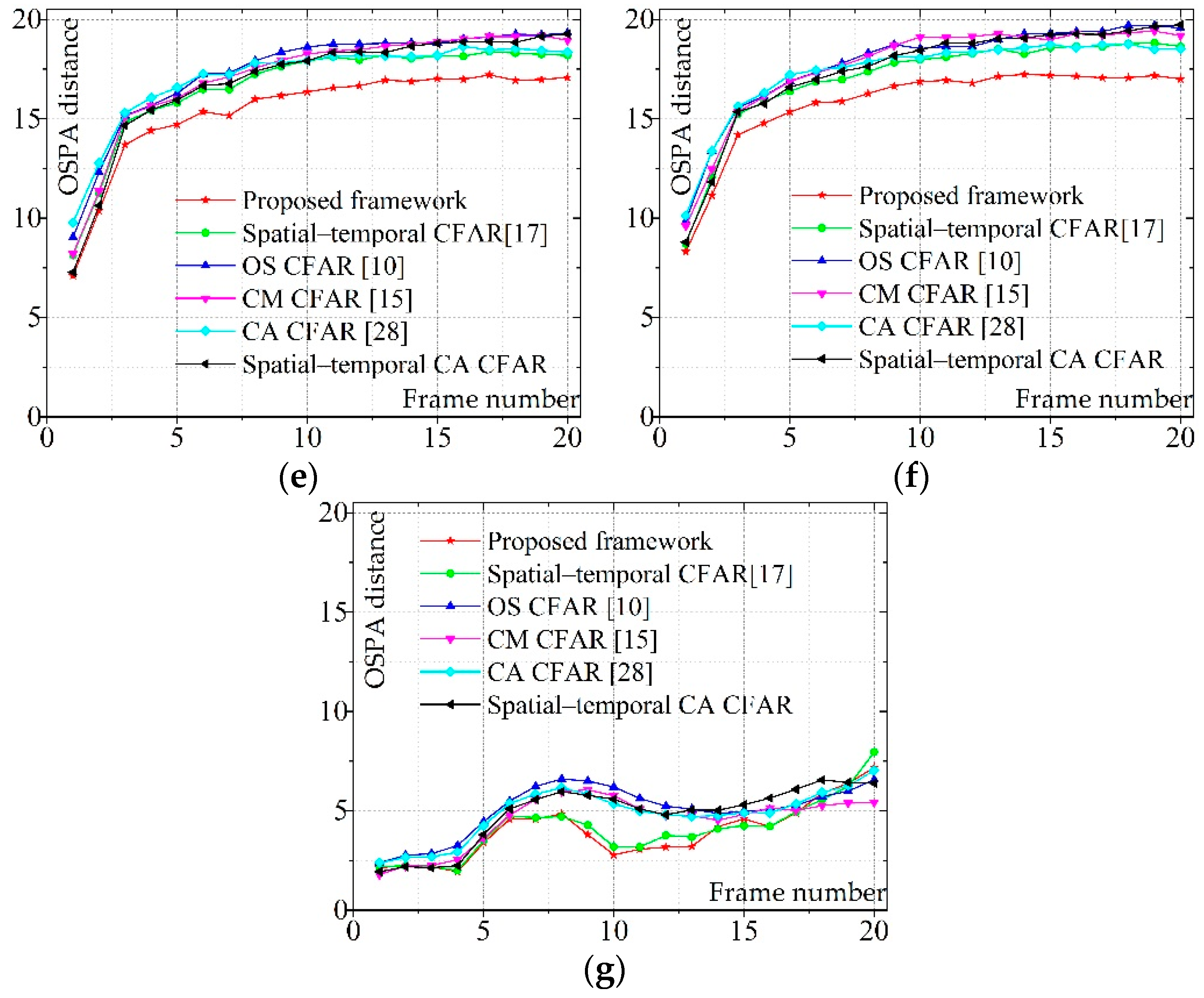
4.2. Synthetic Data
5. Conclusions
Author Contributions
Funding
Conflicts of Interest
References
- Granstrom, K.; Lundquist, C.; Orguner, O. Extended Target Tracking Using a Gaussian-Mixture PHD Filter. IEEE Trans. Aerosp. Electron. Syst. 2012, 48, 3268–3286. [Google Scholar] [CrossRef]
- Orguner, U.; Lundquist, C.; Granström, K. Extended target tracking with a cardinalized probability hypothesis density filter. In Proceedings of the 14th International Conference on Information Fusion, Chicago, IL, USA, 5–8 July 2011. [Google Scholar]
- Granstrom, K.; Orguner, U. On Spawning and Combination of Extended/Group Targets Modeled with Random Matrices. IEEE Trans. Signal Process. 2013, 61, 678–692. [Google Scholar] [CrossRef]
- Granström, K.; Antonio, N.; Braca, P. Gamma Gaussian Inverse Wishart Probability Hypothesis Density for Extended Target Tracking Using X-Band Marine Radar Data. IEEE Trans. Geosci. Remote Sens. 2015, 12, 6617–6631. [Google Scholar] [CrossRef]
- Lundquist, C.; Granström, K.; Orguner, U. An Extended Target CPHD Filter and a Gamma Gaussian Inverse Wishart Implementation. IEEE J. Sel. Top. Signal Process. 2013, 7, 472–483. [Google Scholar] [CrossRef]
- Yan, B.; Xu, N.; Zhao, W.B.; Xu, L.P. A Three-Dimensional Hough Transform-Based Track-Before-Detect Technique for Detecting Extended Targets in Strong Clutter Backgrounds. Sensors 2019, 19, 881. [Google Scholar] [CrossRef]
- Yan, B.; Xu, L.P.; Li, M.Q.; Yan, J.Z.H. A Track-Before-Detect Algorithm Based on Dynamic Programming for Multi-Extended-Targets Detection. IET Signal Process. 2017, 11, 674–686. [Google Scholar] [CrossRef]
- Yan, B.; Zhao, X.Y.; Xu, N.; Chen, Y.; Zhao, W.B. A Grey Wolf Optimization-based Track-Before-Detect Method for Maneuvering Extended Target Detection and Tracking. Sensors 2019, 19, 1577. [Google Scholar] [CrossRef]
- Wang, X.; Li, T.; Sun, S.; Corchado, J.M. A Survey of Recent Advances in Particle Filters and Remaining Challenges for Multitarget Tracking. Sensors 2017, 17, 2707. [Google Scholar] [CrossRef]
- Levanon, N.; Shor, M. Order statistics CFAR for Weibull background. IEE F Radar Signal Process. 1990, 137, 157–162. [Google Scholar] [CrossRef]
- Wang, C.; Bi, F.; Zhang, W.; Chen, L. An intensity-space domain CFAR method for ship detection in HR-SAR images. IEEE Geosci. Remote Sens. Lett. 2017, 99, 1–5. [Google Scholar] [CrossRef]
- Dai, H.; Du, L.; Wang, Y.; Wang, Z. A modified CFAR algorithm based on object proposals for ship target detection in SAR images. IEEE Geosci. Remote Sens. Lett. 2016, 99, 1–5. [Google Scholar] [CrossRef]
- Gao, G.; Shi, G. CFAR ship detection in nonhomogeneous sea clutter using polarimetric SAR data based on the notch filter. IEEE Trans. Geosci. Remote Sens. 2017, 99, 1–14. [Google Scholar] [CrossRef]
- Conte, E.; Lops, M. Clutter-map CFAR detection for range-spread targets in non-gaussian clutter. I. system design. IEEE Trans. Aerosp. Electron. Syst. 1997, 33, 432–443. [Google Scholar] [CrossRef]
- Zhang, R.L.; Sheng, W.X.; Ma, X.F.; Han, Y.B. Clutter map CFAR detector based on maximal resolution cell. Signal Image Video Process. 2015, 9, 1–12. [Google Scholar] [CrossRef]
- Li, Y.; Zhang, Y.; Yu, J.G.; Tan, Y.; Tian, J.; Ma, J. A novel spatio-temporal saliency approach for robust dim moving target detection from airborne infrared image sequences. Inf. Sci. 2016, 369(C), 548–563. [Google Scholar] [CrossRef]
- Deng, L.; Zhu, H.; Tao, C.; Wei, Y. Infrared moving point target detection based on spatial–temporal local contrast filter. Infrared Phys. Technol. 2016, 76, 168–173. [Google Scholar] [CrossRef]
- Xi, T.; Zhao, W.; Wang, H.; Lin, W. Salient object detection with spatiotemporal background priors for video. IEEE Trans. Image Process. 2017, 26, 3425–3436. [Google Scholar] [CrossRef]
- Yan, B.; Xu, L.P.; Zhao, K.; Yan, J.Z.H. An efficient plot fusion method for high resolution radar based on contour tracking algorithm. Int. J. Antennas Propag. 2016. [Google Scholar] [CrossRef]
- Yan, B.; Xu, L.P.; Yan, J.Z.H.; Li, C. An efficient extended target detection method based on region growing and contour tracking algorithm. Proc. Inst. Mech. Eng. Part G- J. Aerosp. Eng. 2018, 232, 825–836. [Google Scholar] [CrossRef]
- Yan, B.; Xu, L.P.; Yang, Y.; Li, C. Improved plot fusion method for dynamic programming based track before detect algorithm. AEU Int. J. Electron. Commun. 2017, 74, 31–43. [Google Scholar] [CrossRef]
- Yan, B.; Xu, N.; Xu, L.P.; Li, M.Q.; Cheng, P. Improved multilevel thresholding plot fusion method using the rain algorithm for the detection of closely extended targets. IET Signal Process. 2019, (in press). [CrossRef]
- Sun, L.; Li, X.R.; Lan, J. Modeling of extended objects based on support functions and extended Gaussian images for target tracking. IEEE Trans. Aerosp. Electron. Syst. 2014, 50, 3021–3035. [Google Scholar] [CrossRef]
- Sutour, C.; Petitjean, J.; Watts, S.; Quellec, J.M. Analysis of K-distributed sea clutter and thermal noise in high range and Doppler resolution radar data. In Proceedings of the 2013 IEEE Radar Conference (RadarCon13), Ottawa, ON, Canada, 29 April–3 May 2013; pp. 1–4. [Google Scholar]
- Watts, S. Radar detection prediction in K-distributed sea clutter and thermal noise. IEEE Trans. Aerosp. Electron. Syst. 1987, 23, 40–45. [Google Scholar] [CrossRef]
- Roy, L.P.; Kumar, R.V.R. Accurate K-Distributed Clutter Model for Scanning Radar Application. IET Radar Sonar Navig. 2010, 4, 158–167. [Google Scholar] [CrossRef]
- Vivone, G.; Braca, P.; Errasti-Alcala, B. Extended target tracking applied to X-band marine radar data. In Proceedings of the OCEANS 2015, Genoa, Italy, 18–21 May 2015; pp. 1–6. [Google Scholar]
- Watts, S. The Performance of Cell-Averageing CFAR Systems in Sea Clutter. In Proceedings of the Record of the IEEE 2000 International Radar Conference, Alexandria, VA, USA, 12 May 2000; pp. 398–403. [Google Scholar]
- Ristic, B.; Vo, B.N.; Clark, D. Performance evaluation of multi-target tracking using the OSPA metric. In Proceedings of the 13th International Conference on Information Fusion, Edinburgh, UK, 26–29 July 2010; pp. 1–7. [Google Scholar]


| Parameter | Value |
|---|---|
| 3dB azimuth beam width | 0.94° |
| Number of bins in range axis (NR) | 8192 |
| Number of bins in range axis (NA) | 8192 |
| Angular Precision | 0.0439° |
| Range Resolution | 6(m) |
| Central frequency | 1.35(GHz) |
| Rotating speed of antenna | π/5(°/s) |
| The Quantity of Cells for One Threshold | The Value of the Quantity | The Total Number of Employed Cells | |
|---|---|---|---|
| The proposed framework | a × b × c | 440 | 8.8 × NR × NA |
| Spatiotemporal CFAR [17] | (m + 2d1) × (n + 2d2)-m × n + p | 293 | 293 × NR × NA |
| OS CFAR [10] | (m + 2d1) × (n + 2d2)-m × n | 278 | 278 × NR × NA |
| CM CFAR [15] | p | 15 | 15 × NR × NA |
| CA CFAR [28] | (m + 2d1) × (n + 2d2)-m × n | 278 | 278 × NR × NA |
| Spatiotemporal CA CFAR | (m + 2d1) × (n + 2d2) × p-m × n | 5052 | 5052 × NR × NA |
| In theory | In the Experiment | |
|---|---|---|
| The proposed framework | NR × NA + (NR/dR) × (NA/dA) × (c-1) | 1.14 NR × NA |
| Spatiotemporal CFAR [17] | NR × NA × p | 15 NR × NA |
| OS CFAR [10] | NR × NA | NR × NA |
| CM CFAR [15] | NR × NA × p | 15 NR × NA |
| CA CFAR [28] | NR × NA | NR × NA |
| Spatiotemporal CA CFAR | NR × NA × p | 15 NR × NA |
| Scenario 1 | Scenario 2 | |
|---|---|---|
| The proposed framework | 4.76 | 4.97 |
| Spatiotemporal CFAR [17] | 220.01 | 219.19 |
| OS CFAR [10] | 3213.15 | 8274.43 |
| CM CFAR [15] | 256.18 | 260.58 |
| CA CFAR [28] | 61.77 | 63.26 |
| Spatiotemporal CA CFAR | 467.96 | 467.56 |
| Group 1 | Group 2 | Group 3 | Group 4 | Group 5 | Group 6 | Group 0 | |
|---|---|---|---|---|---|---|---|
| The proposed framework | 14.4 | 14.67 | 14.96 | 15.07 | 15.43 | 15.8 | 3.97 |
| Spatiotemporal CFAR [17] | 14.59 | 15.35 | 15.88 | 16 | 16.65 | 17.03 | 4.08 |
| OS CFAR [10] | 15.5 | 15.97 | 16.33 | 16.83 | 17.4 | 17.76 | 5.06 |
| CM CFAR [15] | 14.84 | 15.34 | 15.94 | 16.5 | 17.14 | 17.67 | 4.54 |
| CA CFAR [28] | 14.83 | 15.45 | 15.9 | 16.51 | 17.09 | 17.37 | 4.86 |
| Spatiotemporal CA CFAR | 15.6 | 15.81 | 15.97 | 16.4 | 16.9 | 17.47 | 4.84 |
| Group 1 | Group 2 | Group 3 | Group 4 | Group 5 | Group 6 | Group 0 | |
|---|---|---|---|---|---|---|---|
| The proposed framework | 0.49 | 0.43 | 0.39 | 0.35 | 0.37 | 0.38 | 0.35 |
| Spatiotemporal CFAR [17] | 61.36 | 61.68 | 62.06 | 62.11 | 61.84 | 62.39 | 55.6 |
| OS CFAR [10] | 5041.27 | 4993.38 | 5267.96 | 5272.79 | 5319.96 | 5337.25 | 4710.06 |
| CM CFAR [15] | 150.09 | 148.54 | 147.95 | 149.52 | 148.38 | 147.67 | 133.54 |
| CA CFAR [28] | 37.64 | 37.68 | 38.11 | 38.08 | 38.04 | 38.08 | 34.12 |
| Spatiotemporal CA CFAR | 400.43 | 397.42 | 402.07 | 400.77 | 383.4 | 384 | 355.58 |
© 2019 by the authors. Licensee MDPI, Basel, Switzerland. This article is an open access article distributed under the terms and conditions of the Creative Commons Attribution (CC BY) license (http://creativecommons.org/licenses/by/4.0/).
Share and Cite
Yan, B.; Xu, N.; Zhao, W.; Li, M.; Xu, L. An Efficient Extended Targets Detection Framework Based on Sampling and Spatio-Temporal Detection. Sensors 2019, 19, 2912. https://doi.org/10.3390/s19132912
Yan B, Xu N, Zhao W, Li M, Xu L. An Efficient Extended Targets Detection Framework Based on Sampling and Spatio-Temporal Detection. Sensors. 2019; 19(13):2912. https://doi.org/10.3390/s19132912
Chicago/Turabian StyleYan, Bo, Na Xu, Wenbo Zhao, Muqing Li, and Luping Xu. 2019. "An Efficient Extended Targets Detection Framework Based on Sampling and Spatio-Temporal Detection" Sensors 19, no. 13: 2912. https://doi.org/10.3390/s19132912
APA StyleYan, B., Xu, N., Zhao, W., Li, M., & Xu, L. (2019). An Efficient Extended Targets Detection Framework Based on Sampling and Spatio-Temporal Detection. Sensors, 19(13), 2912. https://doi.org/10.3390/s19132912