Low-Power Distributed Data Flow Anomaly-Monitoring Technology for Industrial Internet of Things

Abstract

In recent years, the industrial use of the internet of things (IoT) has been constantly growing and is now widespread. Wireless sensor networks (WSNs) are a fundamental technology that has enabled such prevalent adoption of IoT in industry. WSNs can connect IoT sensors and monitor the working conditions of such sensors and of the overall environment, as well as detect unexpected system events in a timely and accurate manner. Monitoring large amounts of unstructured data generated by IoT devices and collected by the big-data analytics systems is a challenging task. Furthermore, detecting anomalies within the vast amount of data collected in real time by a centralized monitoring system is an even bigger challenge. In the context of the industrial use of the IoT, solutions for monitoring anomalies in distributed data flow need to be explored. In this paper, a low-power distributed data flow anomaly-monitoring model (LP-DDAM) is proposed to mitigate the communication overhead problem. As the data flow monitoring system is only interested in anomalies, which are rare, and the relationship among objects in terms of the size of their attribute values remains stable within any specific period of time, LP-DDAM integrates multiple objects as a complete set for processing, makes full use of the relationship among the objects, selects only one “representative” object for continuous monitoring, establishes certain constraints to ensure correctness, and reduces communication overheads by maintaining the overheads of constraints in exchange for a reduction in the number of monitored objects. Experiments on real data sets show that LP-DDAM can reduce communication overheads by approximately 70% when compared to an equivalent method that continuously monitors all objects under the same conditions.

1. Introduction

The wireless sensor network in the front-end of the industrial internet of things (IoT) often consists of a large number of distributed sensors, where the monitored data are continuously transmitted to the master control node in the form of data flow. The monitoring of the overall state of the system is often determined collectively by the state of each sensor [1,2]. This process is described as monitoring of anomalies in distributed data flows. For example, for applications such as asset and inventory management in the industrial IoT [3,4], or monitoring of power consumption in industrial production, each sensor node monitors data in real time and continuously aggregates the monitored data to a master monitoring node, which will then identify whether the overall situation of the system has exceeded a previously defined security threshold. Due to the largely spread and often hazardous sensor locations in various applications and the cost limitation of sensor nodes in wireless sensor networks, power consumption is often the main factor limiting the performance of an IoT system. Therefore, it is of great significance to study the low-power anomaly-monitoring solutions in distributed data flows for the industrial IoTs [5,6].

To provide a solution on monitoring anomalies in distributed data flows in the industrial IoT when the focus is on reducing the communication overheads and power consumption, a low-power distributed data flow anomaly-monitoring model (LP-DDAM) implementing an algorithm that integrates multiple sets of monitored objects into a single and complete set after fully considering the relationships among objects is presented. In the industrial IoT, sensors are often divided into regions, such as sensors in the warehouse management and monitoring system. Whole system includes multiple warehouses distributed throughout the country, and there are several sensors distributed in each warehouse. The traditional method is that each sensor communicates with the system’s master control node in real time to monitor anomalies. The LP-DDAM method can treat multiple monitored objects in the same region as a whole, and makes full use of the relationship among objects, so that only one representative object needs to communicate with the master control node. The communication overhead is greatly reduced, and the power consumption of sensors except the representative object is also reduced.

LP-DDAM method selects the objects with the largest global values as a set of representative objects among all the objects that may or may not exceed the predefined threshold value. Local adjustment on each representative object factor is applied and local constraints are set up to ensure the correctness of the continuous monitoring process. The continuous monitoring of multiple objects is replaced by monitoring the representative object as well as the local constraints. Only when local constraints are broken, communication and parameter adjustments are needed to reconstruct the local monitoring process. The proposed algorithms, adjustment process and adjustment factor allocation strategy are described in detail in Section 3. In Section 4, the correctness of the algorithm is proved and the extended application of this algorithm in a variety of situations is studied. Experiments on real data sets are explained in Section 5. The results show that the use of the LP-DDAM model can effectively reduce communication overheads in monitoring of distributed data flows to 70% under the same conditions. We conclude the paper and point out future directions in Section 6.

2. Background

Data flow anomaly monitoring has been a very active research field since it was proposed [7,8,9,10], and has been widely used in network security, industrial control, online monitoring and real-time online services [11,12,13,14,15].

For distributed data flow anomaly monitoring, Dilman et al. [16] first put forward the idea of reducing communication overheads. By combining event reporting with rotational monitoring, they proposed two methods, i.e., the simple-value method and the simple-rate method, to reduce communication overheads. In their methods, the remote node no longer monitored the local value but the changes of the local value to reduce the communication overheads. Kale et al. [17] used the trigger method to study threshold monitoring, proposed five evaluation parameters to measure the performance of the algorithm and provided many potential solutions, such as the statistical probability-based method, the global distributed hash table method, and others. Sun et al. [18], to meet the needs of distributed data flow monitoring in smart cities in the future, studied the topic of distributed data flow monitoring from two different perspectives: improving communication efficiency and data privacy protection. In their research, each remote node was assigned multiple local thresholds, representing different “grades”. The centralized nodes only needed to know the “grade” where each local value was located to estimate the global value that would satisfy the accuracy requirement, according to its upper and lower bounds, thus considerably reducing the communication overheads. Macker et al. [19] studied the top-K problem in distributed data flow monitoring and used the filter to reduce the communication between distributed data flow monitoring nodes and primary nodes. Wang et al. [20] studied the anomaly detection method of distributed data flow in vehicle-mounted communication systems, and adopted the method of pre-learning to predict the status of subsequent data flows to reduce communication overheads and improve accuracy. Sadeghioon et al. [21] studied real-time anomaly detection based on temperature and pressure data from real-time sensors in water pipeline monitoring systems. They proposed the methods of dividing and adjusting local thresholds in distributed data flow monitoring, including uniform division, proportional division, static thresholds and dynamic thresholds. They verified the effectiveness of their proposed methods through a large number of experimental analyses.

3. Low-Power Distributed Dataflow Anomaly Monitoring Model

3.1. Model Description

In the industrial IoT, the problem of distributed data flow anomaly monitoring is described as follows: the system consists of m monitored objects O_i (i = 1, …, m), n remote monitoring nodes N_j (j = 1, …, n) and a centralized node N₀. V_i,j represents the monitored local value of the object O_i on the remote monitoring node N_j, so the global value of each object is $V_i={\displaystyle {\sum }_j{V}_{i,j}}$. Each remote node monitors the local data flow S_j, and the new tuple <O_i, N_j, t, V_i,j,t> causes the continuous change of V_i,j as V_i,j = V_i,j + V_i,j,t. The system monitors the anomaly continuously on N₀ by identifying which object’s global value exceeds the threshold T in real time. For each object O_i whose value V_i exceeds the threshold T_i, the approximate value V_i’, which satisfies the pre-specified precision constraint, is obtained.

When monitoring anomalies in distributed data flows, users are often interested in anomalies (i.e., those objects that exceed the threshold) only, while data indicating normal behaviors do not need to be recorded constantly. Therefore, the definition of monitoring of anomalies in distributed data flows in a broader sense is given as follows:

Definition 1.

Approximate threshold monitoring. For any given threshold T and precision constraint parameter δ, the approximate monitoring value V_i’ for object O_i satisfies the following formulas:

$$\begin{array}{l}0\le V_i^{\prime }<T\mathrm{when}{V}_i<T\\ \left|V_i-V_i^{\prime }\right|\le \delta \mathrm{when}{V}_i\ge T\end{array}$$

(1)

where$V_i={\displaystyle {\sum }_j{V}_j}$.

That is, when a global value V_i for object O_i is small, the user is not interested in its specific value other than that it is below the threshold. Only when the global value exceeds the threshold T, its specific value within precision δ is required to be tracked.

Assessment of the values of the threshold relies on global information. However, each monitoring node can only observe its local data. In industrial IoT scenarios, the remote sensor nodes for distributed monitoring are limited by their environment, so their power consumption and communication overheads must be considered. Obviously, if all information about node changes is transmitted to N₀, the monitoring will create vast amount of network overheads. Monitoring by the periodic snapshot acquisition method usually presents periodic outbursts of oscillation of network traffic as well, and a compromise between snapshot frequency and communication overheads must be considered: excessive high frequency will generate large network overheads, while a frequency that is too low will lead to a delay or even loss of reporting on abnormal events. Therefore, the challenge is to reduce communication overheads while still ensuring the correctness of the results and timely response to abnormal events.

3.2. Overview of the Model

First, the LP-DDAM model we propose is based on the following two observations:

Observation 1. The relationships between the global values V_i for different objects are stable during a short period of time.

Observation 2. In most cases, the global value V_i of an object does not exceed a threshold T.

Observation 1 indicates that in the industrial IoT, the relationship between the global values of each monitored object will not change dramatically during any given short period of time. Here is an example on monitoring of power consumption in industrial production [22]: for a given period of time, the power consumption of the lathe producing part 1 on a certain node is always higher than that of the lathe producing part 2. Observation 2 suggests that there exists an anomaly when the monitored event value exceeds a given threshold. Therefore, in general, an object stays longer in the normal state than in the abnormal state, in other words, at any given point in time, majority of the monitored objects are in normal state while minority are in abnormal state (when object value exceeds a given threshold). Based on these two observations, a method to reduce power consumption and communication overheads is proposed when monitoring multiple distributed data flows simultaneously. The overall idea is as follows:

(1)

For all objects that exceed each of their threshold T_i, the existing uniform threshold assignment (UTA) is used to continuously track approximate values satisfying accuracy constraints, to ensure that the monitored value of each object satisfies the requirements set forth in Definition 1.

(2)

For most objects that do not exceed their corresponding T_i, only the object O_max with the largest global value is selected as the representative value for continuous tracking.

(3)

Through the “adjustment factor” parameter, we adjust the local value of the object O_max to be the largest on each remote node to ensure that other objects can be represented by O_max, that is, if O_max does not exceed the threshold, other objects do not exceed the threshold either.

(4)

Continuous monitoring of multiple objects is transformed into monitoring of O_max keeping its local maximum constraints. Communication is required only when the constraints are no longer satisfied due to the arrival of new data, thus reducing the communication overheads.

Definition 2.

Representative object. $\forall O_j\ne O_i$, $V_i\ge V_j$, that is, if O_i has the largest global value, it is called the representative object, which is represented by O_max.

Definition 3.

Adjustment factors. An adjustment factor ε_i,j is assigned to each node N_j (j = 0, …, n) for each object O_i, satisfying the following constraints:

$$\begin{array}{l}\left(1\right)\forall O_i,{\displaystyle \sum _{j=0}^n{\epsilon }_{i,j}}=0\\ (2)\forall N_j(1\le j\le \mathrm{n}),and\forall O_i\ne O_{\max },V_{\max ,j}+{\epsilon }_{\max ,j}\ge V_{i,j}+{\epsilon }_{i,j}\end{array}$$

(2)

Constraint (1) requires the sum of all adjustment factors of each object to be zero, so it will not affect the correctness of the global value. Constraint (2) requires the representative object to have the largest local value on each remote node after the adjustment factors are added.

The symbols used here and their meanings are shown in

Table 1. List of symbols.

Symbols	Meaning	Symbols	Meaning
U	Universe of data objects	Vi,j	Partial data value of Oi on node Nj
T	User-specified threshold	εi,j	Adjustment factor for Vi,j
Oi	Data object (i = 1, …, m)	Nc	Remote node violating the local constrain
Omax	The representative object	C	Set of objects violating the local constrain
N0	Central coordinator node	R	Set of nodes participating in resolution
Nj	Remote node (j = 1, …, n)	N	Set of all nodes
Sj	local data flow in Nj	Bj	Border value from node Nj
Vi	Global value for object Oi	OT	Set of objects that exceed the threshold T
δ	precision constraint parameter	V′	approximate monitoring value

.

3.3. Model Description

3.3.1. Framework of Algorithms for the Model

The low-power distributed data flow anomaly-monitoring model (LP-DDAM) is shown as Algorithm 1. For all object sets OT that exceed the threshold T, the existing UTA method is used for continuous approximate monitoring. Therefore, for the sake of simplicity of description, it is assumed that the set of objects that do not exceed the threshold is U, and only the unified monitoring method of these objects is considered. This concept is presented below as the LP-DDAM algorithm. The core of the LP-DDAM algorithm is to make the local value V_max,j + ε_max,j of the representative object O_max appear to be the maximum on each monitoring node by adjusting the factor. Therefore, as long as this constraint is satisfied, the method of continuous monitoring of O_max can be adopted to replace that of monitoring all objects: as long as the global value of O_max does not exceed T, other objects will certainly not exceed T. When O_max exceeds T or when the global value of an object that previously exceeded the threshold is less than T at a certain point of time, the LP-DDAM algorithm needs to be invoked again to select the representative object and allocate adjustment factors.

Algorithm 1. Low-power distributed data flow anomaly-monitoring model (LP-DDAM).
1	N0 obtains the initial value Vi,j of each object, and selects the object Omax with the largest global value as the representative for continuous monitoring. Then, the reallocation algorithm (defined below in Section 3.3.3) is used to assign the adjustment factors εi,j on each node Nj (j = 0, …, n) for each object Oi (i =1, …, m) in U, and then they are sent to the corresponding Nj.
2	Each monitoring node Nj (j = 1, …, n) monitors the local data flow Sj separately:
3	While (1)
4	Read the data in Sj <Oi, Nj, t, Vi,j,t>
5	Vi,j = Vi,j + Vi,j,t
6	If $\exists O_c\in U,O_c\ne O_{\max }$, Vmax,j + εmax,j ≤ Vc,j + εc,j
7	Use the “Adjustment algorithm” to adjust the system
8	If the centralized node N0 finds that Vmax exceeds the threshold, then we set OT = OT + {Omax}, and U = U − {Omax}, and then the LP-DDAM algorithm is again used.
9	If the object that previously exceeded the threshold is below the threshold at a certain time, the third step in the resolution process is called for adjustment.

3.3.2. Adjustment Process

At a certain point, when the remote node N_c finds that local constraints are broken, it needs to call the “Adjustment process” for adjust the system (Lines 6 and 7 of the LP-DDAM algorithm). Definitions of several terms are given next.

Definition 4.

Conflict sets. Conflict sets are sets of objects that violate constraints, that is, $C=\left\{O_i|V_{\mathrm{i},\mathrm{c}}+{\epsilon }_{i,c}>V_{\max ,c}+{\epsilon }_{\max ,c}\right\}$ including all objects with local values greater than O_max on the N_c node.

Definition 5.

Lower bound. The conflict set is on the lower bound $B_j=\max \{V_{i,j}+{\epsilon }_{i,j}|O_i\in U-C-O_{\max }\}$ on the node N_j.

The adjustment process is described as Algorithm 2. When allocating adjustment factors, to avoid a global adjustment every time the constraint is broken, we do not allocate all “surpluses” to remote nodes; instead, a part is reserved on N₀, marked as ε_i,0, and the lower boundary $B_0=\max \left\{{\epsilon }_{i,0}|O_i\in U-C-O_{\max }\right\}$ on N₀ is defined. When N_c sends the reconstruction constraint request, the first step is to determine whether the adjustment can be completed through ε_i,0. If it can, the adjustment only occurs between N₀ and N_c; otherwise, it is necessary to obtain the values of the related objects from other remote monitoring nodes for global allocation and adjustment.

The lower bound B_j is a parameter introduced to reduce the traffic of each adjustment. It represents the upper bound of local values of objects other than conflict sets C and O_max on the node N_j. By using this parameter, the transfer of a large number of local values of objects is avoided.

Algorithm 2. Adjustment.
1	Nc sends reconstruction constraint requests to N0, including the conflict set C, the monitoring values of objects in C on Nc, Vmax,c and the lower bound Bc.
2	N0 carries out a validity test: If $\forall O_c\in C$,$V_{\max ,c}+{\epsilon }_{\max ,0}+{\epsilon }_{\max ,c}\ge V_{c,c}+{\epsilon }_{c,0}+{\epsilon }_{c,c}$, then the validity test is successful. Call the “reallocation algorithm” to recalculate the adjustment factors of Nc and N0, and then the new adjustment factors are sent to Nc. At this point, the resolution process ends. If the validity test fails, the third step is executed.
3	N0 obtains the monitored values of objects and Omax in set C from each node $N_{\mathrm{j}}(1\le j\le n,j\ne c)$ and the lower bound Bj, and then identifies the new representative object O’max according to the aggregated values of objects. Finally, it calls the reallocation function to recalculate the adjustment factors of all nodes, and sends O’max and new adjustment factors to each monitoring node.

3.3.3. Adjustment Factor Allocation

The LP-DDAM algorithm calls the reallocation function to calculate the adjustment factor in the initialization stage, as well as the second and third stages in the resolution process, but the adjustment factor is calculated only between N_c and N₀ in the second stage of the resolution process, while the adjustment factors on all nodes are calculated in the initialization stage and the third stage of the resolution process. The concepts of partially aggregated values of participated nodes set N and objects on N are defined next.

Definition 6.

Participated nodes set. In the second stage of the resolution process, the participated nodes set is N = {N_c,N₀}; in other cases, N = {N_i|i = 0, …, n}.

Definition 7.

Partial aggregation values. The partial aggregation value V_iN of object O_i on N, and the partial aggregation value B_N on the lower bound are defined as follows:

$$\begin{array}{l}{\mathrm{V}}_{iN}={\epsilon }_{i,0}+{\displaystyle {\sum }_{1\le j\le n,N_j\in N}(V_{i,j}+{\epsilon }_{i,j})}\\ {\mathrm{B}}_N={\displaystyle {\sum }_{0\le j\le n,N_j\in N}{B}_j}\end{array}$$

(3)

Definition 8.

Allocation factors. When calculating the adjustment factors, an allocation factor F_j is assigned to each node, representing the allocation strategy of the adjustment factor. The allocation factor satisfies the following constraints:

(1)

$0\le F_j\le 1$;

(2)

If $N_j\notin N$, F_j = 0;

(3)

${\displaystyle \sum _{j=0}^n{F}_j}=1$

The description of the process of adjustment factor allocation is shown in Algorithm 3. It can be seen that the reallocation process first approximatively calculates the “surplus” of each object according to the lower bound, and then distributes the “surplus” between the remote node and the centralized node according to a certain strategy, so that the difference between the adjusted object value and the lower bound is F_jλ_i. The different assignment of allocation factors reflects the difference of adjustment factors in allocation strategies. Generally speaking, the allocation factor F₀ on N₀ needs to be specified separately to allocate large “surplus” for local adjustment in phase 2 of the resolution process. The remaining “surplus” can be allocated among N_j (j = 1, …, n) nodes according to a certain strategy. The choice of F₀ needs to consider the balance between the adjustment frequency and the communication required for each adjustment: the larger F₀ is, the more adjustments are local adjustments, so the required amount of communication for each adjustment is small. However, the larger the F₀, the stricter the constraints of the remote nodes are, and the easier it is to violate the local constraints, that is, the more frequent the resolution adjustment will be. Conversely, the smaller the F₀ is, the smaller is the chance for remote nodes to break constraints, but the greater the possibility of global adjustment in phase 3 of the resolution process, that is, the greater the traffic per adjustment.

Algorithm 3. Reallocation
Input: C, N, {Bj}, {Vi,j}, {εi,j}, {Fj}
Output: {ε’i,j }
1	For each object Oi in $R=C\cup \left\{O_{\max }\right\}$, the allocated balance λi is calculated as λi = ViN − BN
2	For each object Oi in R, its new adjustment factor ε’i,j on each node in N is calculated as ε’i,j = Bj − Vi,j + Fjλi

The allocation of F_j (j = 1, …, n) should reflect the distribution of data in different nodes. According to the actual situation, we can choose from the following allocation strategies:

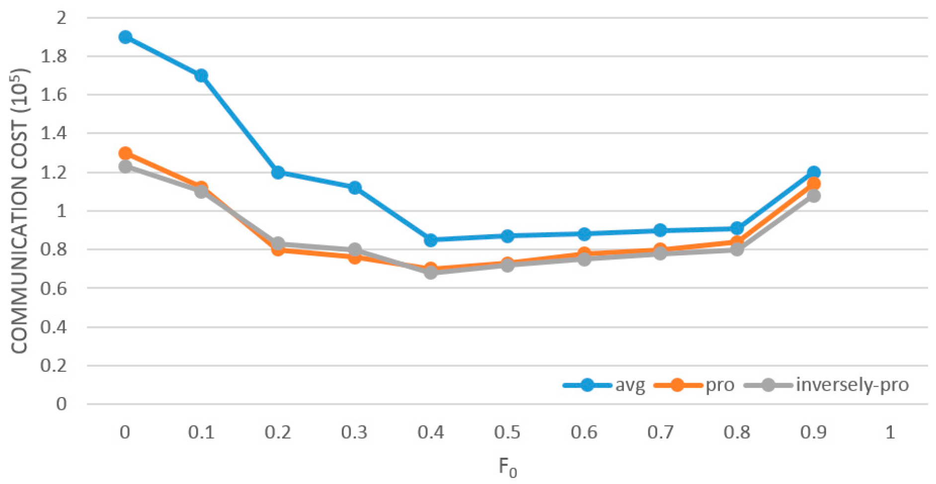
• Average allocation strategy. The “surplus” is allocated equally among remote nodes, i.e., F_j = (1 − F₀)/(|N| − 1).
• Proportional allocation strategy. The allocation of “surplus” is proportional to the lower bound B_j of node N_j, i.e., F_j = (1 − F₀)B_j/(B_N − B₀).
• Inversely proportional allocation strategy. The allocation of “surplus” is inversely proportional to (V_max,j − B_j), i.e., $F_j=(1-F_0)(\frac{1}{\left|N\right|-1}-\frac{V_{\max ,j}-B_j}{V_{\max ,N-\left\{N_0\right\}}-B_N+B_0})$.

4. Analysis and Extension of the Model

4.1. Proof of Correctness of the Proposed Solution

The proof of correctness on the proposed solution is provided below. First, it is assumed that the adjustment calculation takes less time than the tuple arrival interval in the data flow, that is, no new data arrives during the adjustment process. Obviously, the algorithm is correct when all remote nodes satisfy local constraints, so we only need to prove that the two constraints in Definition 3 are still satisfied after the adjustment in the resolution process is completed. This is proved by mathematical induction as follows.

1. LP-DDAM initialization calls only for reallocation adjustment factors. $\forall O_i\notin R$, O_i does not participate in the allocation, so ε_i,j = 0, which obviously satisfies the constraint (1). $\forall O_i\in R$, according to the reallocation algorithm, we obtain the following equation:

$${\displaystyle \sum _{j=0}^n{\epsilon }_{i,j}}={\displaystyle \sum _{j=0}^n{B}_j-V_{i,j}+F_j{\lambda }_i}=B_N-V_{i,N}+{\displaystyle \sum _{j=0}^n{F}_j{\lambda }_i}.$$

(4)

According the constraint (3) of Definition 8 and the definition of λ_i in Line 1 of the reallocation algorithm, ${\displaystyle \sum _{j=0}^n{\epsilon }_{i,j}}=0$ can be obtained.

$\forall N_j(1\le j\le \mathrm{n})$, V_max,j + ε_max,j = B_j + F_jλ_max

$\forall O_i\ne O_{\max }$, if $\forall O_i\notin R$, then ε_i,j = 0. According to the definition of the lower bound, $V_{i,j}\le B_j$, then $V_{\max ,j}+{\epsilon }_{\max ,j}\ge V_{i,j}+{\epsilon }_{i,j}$. $\forall O_i\in R$, (V_max,j + ε_max,j) − (V_i,j + ε_i,j) = (B_j + F_jλ_max) − (B_j + F_jλ_i) = F_j(λ_max − λ_i) = F_j(V_max,N − V_i,N). From the Definitions 2, 7 and 8, it follows that F_j(V_max,N − V_i,N) ≥ 0, so $V_{\max ,j}+{\epsilon }_{\max ,j}\ge V_{i,j}+{\epsilon }_{i,j}$.

Therefore, after LP-DDAM calls the reallocation initialization, the system satisfies the two constraints of Definition 3.

2. If the two constraints of Definition 3 are satisfied on all remote nodes before the local constraints are broken, we then prove that the two constraints are still satisfied after the local constraints are broken and the resolution process is adjusted.

If the resolution process ends after step 2 is implemented, it means that the representative object O_max has not changed and the adjustment only occurs between N₀ and N_c. Therefore, for $\forall N_j\ne N_c$ and $\forall O_i\notin R$ on N_c, the constraints are still satisfied. For $\forall O_c\in C$ participating in the adjustment, it satisfies the condition $V_{\max ,c}+{\epsilon }_{\max ,0}+{\epsilon }_{\max ,c}\ge V_{c,c}+{\epsilon }_{c,0}+{\epsilon }_{c,c}$. Similarly, to the above proof process, the two constraints of Definition 3 can still be satisfied after adjustment.

If the resolution process executes step 3, according to the definition of the lower bound, V_max,c > B_c. For any other nodes $N_j(j\ne c)$ that do not violate local constraints, it is obvious that V_max,j > B_j, so λ_max = V_max,N − B_N > 0. Therefore, whether the new object is the same as the original object or not, the calculated “surplus” based on the lower bound must be positive. The same process can be applied to other proofs. In conclusion, the above method proves the correctness of the algorithms.

4.2. Performance Analysis of the Algorithms

The network traffic of the distributed data flow anomaly monitoring depends on the number of communications between remote nodes and centralized nodes and the size of messages in each communication [23]. On one hand, it is related to data distribution and on the other hand, it is closely related to the selection of algorithm’s parameters. Existing algorithms deal with monitoring of multiple objects independently. Although some methods have been adopted to reduce the communication overheads, in general, the communication overheads of these methods are linearly related to the number of objects m. However, LP-DDAM only selects a representative object to monitor to adjust the additional cost of constraints in exchange for fewer actual monitored objects, so there is no obvious linear relationship between the traffic and the number of monitored objects. In industrial IoT applications, front-end sensors are often large-scale distributed systems, and the number of sensors is large. Communication overheads of the LP-DDAM algorithm will not increase linearly with the number of sensors, which greatly reduces the system’s traffic. Compared with the existing methods, the LP-DDAM algorithm is also affected by different characteristics of data distribution. LP-DDAM is sensitive to the stability of the relationship between monitored objects, while the existing methods (such as the UTA algorithm) are greatly affected by the changes in the span of the object value itself. Therefore, they can complement each other to a certain extent and meet the monitoring needs of data with different distribution characteristics.

4.3. LP-DDAM Model Extension

LP-DDAM assumes that all monitored objects have the same threshold parameter T. However, in real-world scenarios, this hypothesis does not necessarily hold in many cases. For such cases, standardization can be carried out, that is, the threshold of all the objects is considered as 1, and the local value V_i,j is converted into V’_i,j = V_i,j/T_i, where T_i is the corresponding threshold of the object O_i. Correspondingly, the data tuple <O_i, N_j, t, V_i,j,t> becomes <O_i, N_j, t, V_i,j,t/T_i>. Through this standardization change, the LP-DDAM algorithm can deal with the problem of monitoring multiple objects with different thresholds.

If the monitoring value of object O_max on a node drops and leads to the violation of local constraints, the conflict set C may be large. In order to reduce the communication overheads during adjustment, the following improvements can be considered. When a remote node N_j receives data <O_i, N_j, t, V_i,j,t> and finds that the constraint is broken and |C| > Φ (Φ is threshold set by user), V_i,j = V_i,j − V_i,j,t is ordered to cancel the effect of this data on V_i,j. Then, N_j sends a data <O_i, N_j, t, V_i,j,t> to N₀. After N₀ receives it, N₀ sends data <O_i, V_i,j,t> to other nodes. Each remote node N_w (w ≠ j) calculates the size of the conflict set |C_w| caused by V_i,w = V_i,w + V_i,j,t, and sends it to N₀. N₀ selects the node with the smallest |C_w| value as the node whose constraint is broken to rebuild the constraint.

If the approximation problem in Definition1 is slightly extended as follows,

$$\begin{array}{l}0\le V^{\prime }<T\mathrm{when}V<(1+\delta )T\\ \left|V-V^{\prime }\right|\le \delta T\mathrm{when}V\ge (1+\delta )T\end{array}$$

(5)

then the local constraints on LP-DDAM remote nodes (i.e., condition 2 in Definition 3) can be further relaxed as follows: V_i,j + ε_i,j ≤ (1 + δ)(V_max,j + ε_max,j), that is, the local values of other objects can exceed the local values of O_max within a certain range. This is because monitoring O_max with the UTA method can ensure that V_max < T. Therefore ${\displaystyle \sum _{j=0}^n(1+\delta )(V_{\max ,j}+{\epsilon }_{\max ,j})}<(1+\delta )T$, that is, the representation of object O_max can still be guaranteed after relaxing the conditions. As long as the representative object does not exceed the threshold and the local constraints are not broken, the global values of other objects will not exceed (1 + δ)T. Therefore, using this extension of the algorithm can further reduce communication overheads.

5. Experimental Analysis

5.1. Experimental Data

We tested the LP-DDAM algorithm with the industrial IoT monitoring data from Sany Heavy Industry [24]. Sany Heavy Industry is the first enterprise in China that applies the industrial IoT to production process monitoring and equipment management. All large-scale equipment manufactured by Sany Heavy Industry sends its location information, equipment status and other information to the master control platform in real time through a network of sensors. The test data set used in this paper was the data obtained from the equipment power consumption anomaly monitoring system of Sany Heavy Industry. We duplicated the data set of monitored power consumption of 50 kinds of equipment from 10 monitoring nodes in a month, and the system topology is shown in the Figure 1. Among them, O₁~O_m are the monitoring objects. Here we have selected 50 monitoring devices, so m = 50. Node 1~Node n were the monitoring nodes, and we selected 10 distributed monitoring nodes, so n = 10. The test data was the power consumption and temperature anomaly of the monitoring system, the monitoring interval is 5 s and continuous monitoring was performed for 7 × 24 hour. The equipment monitored was distributed in 10 areas, 50 devices in each area, so the data volume per month was (60 × 60/5) × 24 × 30 × 10 × 50, which was about 260 million. We tested the performance of the LP-DDAM algorithm with this data set.

5.2. Experiment Results and Analysis

The purpose of the LP-DDAM technology proposed in this paper was to reduce the communication overheads. Therefore, we tested the influence of various parameters of the LP-DDAM algorithm on the communication overheads and compared the communication overheads with that of the existing algorithms (the classical UTA algorithm was chosen as a comparison).

5.2.1. Influence of Allocation Factor and Allocation Strategy on Communication Overheads

The assignment strategy of the allocation factor F_j(j = 0, …, n) plays the key role in determining the performance of LP-DDAM in reducing communication overheads. Figure 2 shows the system’s communication overheads (T = 2,500,000, δ = 0.001) when F₀ was pre-allocated with different values and the adjustment factor adopts three strategies: average allocation (avg), proportional allocation (pro) and inversely-proportional allocation (inversely-pro). It shows that the value of F₀ had a great impact on the algorithm’s performance in reducing communication overheads. When F₀ was between 0.4 and 0.6, there was a good balance between the frequency of violations of local constraints and the cost of each adjustment. In general, the method of allocating adjustment factors proportionally achieves better effect than the average allocation method because they considered the conditions of data distribution on different nodes, and among the methods of allocating adjustment factors proportionally, the inversely-proportional strategy was slightly better than the proportional strategy. For this reason, the follow-up experiments were conducted with the inversely-proportional allocation strategy.

5.2.2. Influence of Allocation Factor and Thresholds on Communication Overheads

The influence of the value of F₀ on the communication overhead of the algorithm was also related to the monitoring threshold of the system. Therefore, we tested the monitoring threshold from T = 2,000,000 to T = 3,000,000. The test results are shown in the Figure 3. It can be seen that the larger the monitoring threshold is, the smaller the communication overhead of the system is, because the chance of breaking constraint becomes smaller. When the value of F₀ was large, the effect of reducing the communication overhead will be better. On the contrary, when the monitoring threshold was small and the value of F₀ was small, the remote node will have less chance to break the constraint, and its effect will be better. The follow-up experiments were conducted with a fixed T = 2,500,000, and F₀ = 0.5.

5.2.3. Change of Communication Overheads with the Number of Monitored Objects

Figure 4 shows the comparison of traffic between LP-DDAM and UTA (T = 2,500,000, δ = 0.001) on the monitored data set of Sany Heavy Industry’s equipment power consumption as the number of monitored objects increases. The two algorithms are compared under the same conditions. It is clear that the UTA method needs continuous monitoring of each object, so the traffic increases linearly with the number of monitored objects. However, the LP-DDAM method only monitored the representative object continuously while ensuring that the local constraints are not broken, so the required traffic is not significantly affected by the number of objects. Therefore, in the large-scale multi-object monitoring condition, there was a clear advantage of the LP-DDAM method in reducing communication overheads.

5.2.4. Influence of Error Parameters on Reducing Communication Overheads

The influence of accuracy error δ on reduction of communication overheads is shown in Figure 5 (T = 2,500,000). The two algorithms are compared under the same conditions. The larger the δ was, the larger the “grade” width (δT/M) used by the UTA method was. Therefore, the smaller the probability of the change of the object’s “grade” was, the smaller the traffic required by the system was. LP-DDAM used the UTA method to process all objects that exceed the threshold of the representative object, so the communication overheads will decrease with the increase of δ. However, UTA is more sensitive to the change of δ. It can be seen from the figure that when the δ value is small, the traffic required by the UTA method increases sharply. In contrast, the LP-DDAM method changes more smoothly, that is, the LP-DDAM method has more obvious advantages in situations with a smaller δ.

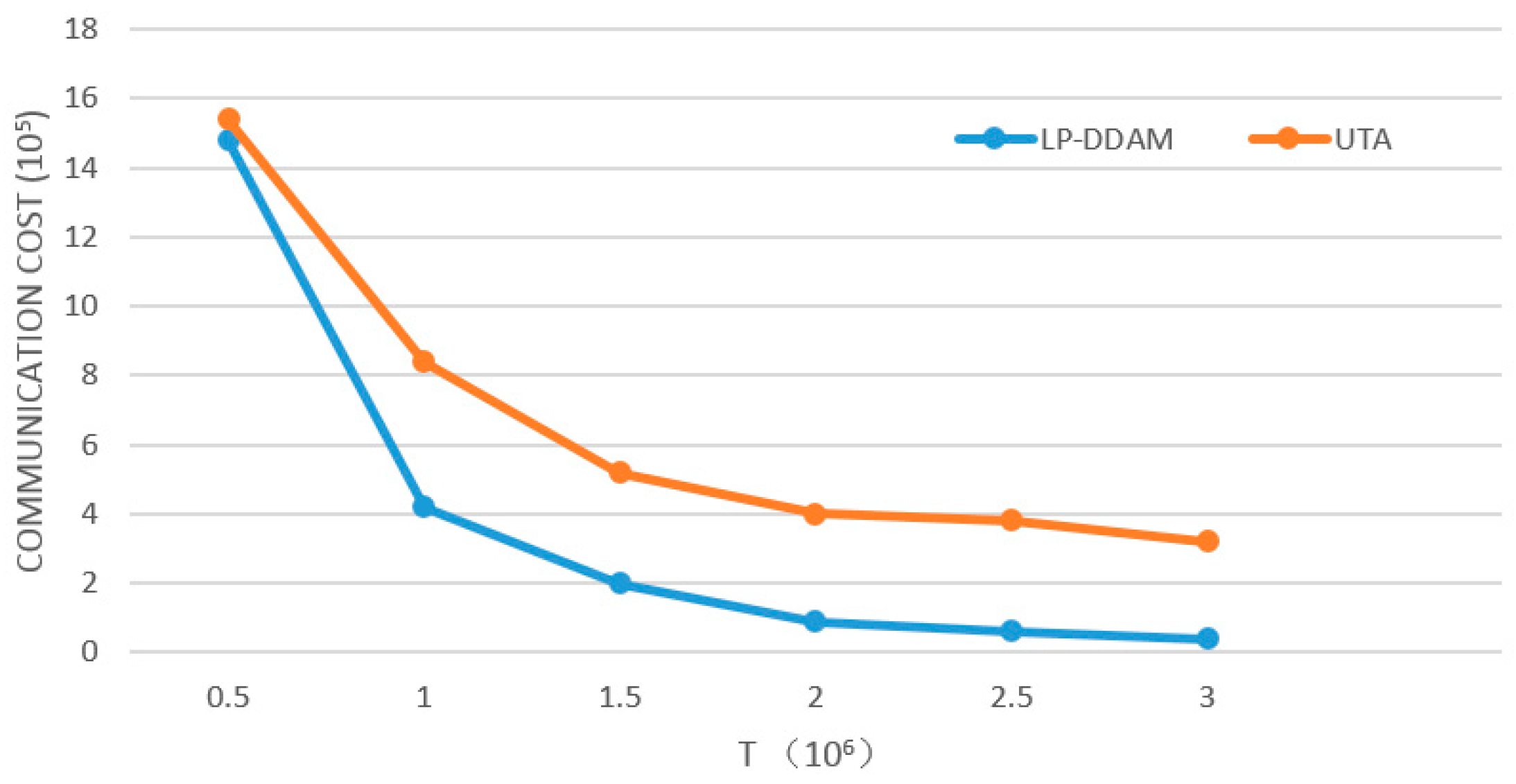
5.2.5. Changes of Communication Overheads with Threshold Parameters

The number of monitored objects is fixed (M = 50), and the threshold T is changed to change the proportion of objects exceeding the threshold to all objects. The effect of threshold parameters on traffic is analyzed, as shown in Figure 6. The two algorithms are compared under the same conditions. LP-DDAM reduces communication overheads mainly by exploring the relationship between objects below the threshold. With the decrease of T, more objects exceed the threshold, and these objects were tracked by the UTA method to obtain approximate solutions to meet the accuracy requirements. In addition, the objects fluctuated repeatedly in the threshold, which called the eighth and ninth lines of the LP-DDAM algorithm to initialize or adjust globally, resulting in larger communication overheads.

Therefore, the lower the value of T was, the smaller the advantage the LP-DDAM method had. In extreme cases where all objects exceed the threshold, the LP-DDAM method transformed into the UTA method. Experiments on two datasets showed that when the global values of more than 60% of the objects were below the threshold, the LP-DDAM method needed less than 30% of the traffic of the UTA method.

6. Conclusions

To provide a feasible solution on monitoring anomalies in distributed data flows in industrial IoT, we introduce a low-power distributed dataflow anomaly-monitoring model in this paper. The model is conceived under the assumption that (1) the monitoring system is only interested in detecting anomalies, which are rare, and (2) the relationship among the objects regarding the size of their attribute values in real-world practice is usually stable over any given period of time. In the proposed solution, multiple objects are integrated in a single whole set, making full use of the relationship between objects. The model selects only one set of “representative” object for continuous monitoring and establishes certain constraints to ensure correctness, that is, other objects can be represented by this “representative object”, or it is guaranteed that the representative object will always have the largest global value. The communication overheads can be reduced because of the reduction in the number of monitored objects. Experiments on real data sets show that LP-DDAM can reduce communication overheads by about 70% comparing with those achieved by using methods running continuous monitoring of each object under the same conditions.

A consequence of using LP-DDAM to reduce communication overheads is the increased costs on computation and storage. In addition, because of the characteristics of the LP-DDAM method, its performance in reducing communication overheads is conditional and not applicable to all distributed data sets. When there is no obvious relationship among the objects in terms of the size of their global values, the “representative object” will be displaced frequently. When the global values of many objects fluctuate frequently around the threshold due to improper selection of threshold parameters, the LP-DDAM model must undergo a great deal of global adjustments, resulting in extra costs that are likely to outweigh the benefits. Therefore, in some special application scenarios where Observation 1 and Observation 2 described in Section 3.2 do not hold, the LP-DDAM approach to reduce communication overheads is likely to fall short of expectations.

This paper does not discuss the security and trustworthiness of the algorithm. In the future work, we will research on the security and trusty of LP-DDAM algorithm. In addition, when the application scenarios where Observation 1 and Observation 2 described in Section 3.2 do not hold, how to reduce the communication overhead is the further research direction.

References

1. Du, X.; Chen, H.H. Security in Wireless Sensor Networks. IEEE Wirel. Commun. Mag. 2008, 15, 60–66. [Google Scholar]
2. Tian, Z.; Su, S.; Shi, W.; Du, X.; Guizani, M.; Yu, X. A Data-driven Model for Future Internet Route Decision Modeling. Future Gener. Comput. Syst. 2019, 95, 212–220. [Google Scholar] [CrossRef]
3. Tian, Z.; Li, M.; Qiu, M.; Sun, Y.; Su, S. Block-DEF: A Secure Digital Evidence System using Blockchain. Inf. Sci. 2019, 491, 151–165. [Google Scholar] [CrossRef]
4. Bhatkar, S.; Chaturvedi, A.; Sekar, R. Dataflow Anomaly Detection. In Proceedings of the 2006 IEEE Symposium on Security & Privacy, Berkeley/Oakland, CA, USA, 21–24 May 2006. [Google Scholar]
5. Hong, Y.; Xu, C.; Su, D.X. Research of Smart Phone Malware Detection Based on Anomaly Data Flow Monitoring. Comput. Secur. 2012, 9, 4. [Google Scholar]
6. Tian, Z.; Shi, W.; Wang, Y.; Zhu, C.; Du, X.; Su, S.; Sun, Y.; Guizani, N. Real Time Lateral Movement Detection based on Evidence Reasoning Network for Edge Computing Environment. IEEE Trans. Ind. Inform. 2019. [Google Scholar] [CrossRef]
7. Xiao, Y.; Rayi, V.; Sun, B.; Du, X.; Hu, F.; Galloway, M. A Survey of Key Management Schemes in Wireless Sensor Networks. J. Comput. Commun. 2007, 30, 2314–2341. [Google Scholar] [CrossRef]
8. Du, X.; Xiao, Y.; Guizani, M.; Chen, H.H. An Effective Key Management Scheme for Heterogeneous Sensor Networks. Ad Hoc Netw. 2007, 5, 24–34. [Google Scholar] [CrossRef]
9. Tan, Q.; Gao, Y.; Shi, J.; Wang, X.; Fang, B.; Tian, Z. Towards a Comprehensive Insight into the Eclipse Attacks of Tor Hidden Services. IEEE Internet Things J. 2018. [Google Scholar] [CrossRef]
10. Xiao, Y.; Du, X.; Zhang, J.; Guizani, S. Internet Protocol Television (IPTV): The Killer Application for the Next Generation Internet. IEEE Commun. Mag. 2007, 45, 126–134. [Google Scholar] [CrossRef]
11. Nirmali, B.; Wickramasinghe, S.; Munasinghe, T.; Amalraj, C.R.J.; Dilum Bandara, H.M.N. Vehicular data acquisition and analytics system for real-time driver behavior monitoring and anomaly detection. In Proceedings of the 2017 IEEE International Conference on Industrial & Information Systems, Peradeniya, Sri Lanka, 15–16 December 2017. [Google Scholar]
12. Qidwai, U.; Chaudhry, J.; Jabbar, S.; Zeeshan, H.M.A.; Janjua, N.; Khalid, S. Using casual reasoning for anomaly detection among ECG live data streams in ubiquitous healthcare monitoring systems. J. Ambient. Intell. Humaniz. Comput. 2018, 1–13. [Google Scholar] [CrossRef]
13. Zhang, C.; Yan, H.; Lee, S.; Shi, J. Multiple profiles sensor-based monitoring and anomaly detection. J. Qual. Technol. 2018, 50, 344–362. [Google Scholar] [CrossRef]
14. Siow, E.; Tiropanis, T.; Hall, W. Analytics for the Internet of Things: A Survey. ACM Comput. Surv. 2018, 1, 1. [Google Scholar] [CrossRef]
15. Fraga-Lamas, P.; Fernández-Caramés, T.M.; Suárez-Albela, M.; Castedo, L.; González-López, M. A Review on Internet of Things for Defense and Public Safety. Sensors 2016, 16, 1644. [Google Scholar] [CrossRef] [PubMed]
16. Dilman, M.; Raz, D. Efficient reactive monitoring. IEEE J. Sel. Areas Commun. (JSAC) 2002, 20, 668–676. [Google Scholar] [CrossRef]
17. Kale, A.; Chaczko, Z. iMuDS: An Internet of Multimodal Data Acquisition and Analysis Systems for Monitoring Urban Waterways. In Proceedings of the 2017 25th International Conference on Systems Engineering, Las Vegas, NV, USA, 22–24 August 2017. [Google Scholar]
18. Sun, J.; Zhang, R.; Zhang, J.; Zhang, Y. PriStream: Privacy-preserving distributed stream monitoring of thresholded PERCENTILE statistics. In Proceedings of the IEEE Infocom 2016—The 35th Annual IEEE International Conference on Computer Communications, San Francisco, CA, USA, 10–14 April 2016. [Google Scholar]
19. Macker, A.; Malatyali, M.; Heide, F.M.A.D. Online Top-k-Position Monitoring of Distributed Data Streams. In Proceedings of the 2015 IEEE International Parallel and Distributed Processing Symposium (IPDPS), Hyderabad, India, 25–29 May 2015. [Google Scholar]
20. Wang, C.; Zhao, Z.; Gong, L.; Zhu, L.; Liu, Z.; Cheng, X. A Distributed Anomaly Detection System for In-Vehicle Network using HTM. IEEE Access 2018, 6, 9091–9098. [Google Scholar] [CrossRef]
21. Sadeghioon, A.M.; Metje, N.; Chapman, D.; Anthony, C. Water pipeline failure detection using distributed relative pressure and temperature measurements and anomaly detection algorithms. Urban Water J. 2018, 15, 287–295. [Google Scholar] [CrossRef] [Green Version]
22. Jiménez, J.M.H.; Nichols, J.A.; Gosevapopstojanova, K.; Prowell, S.; Bridges, R. Malware Detection on General-Purpose Computers Using Power Consumption Monitoring: A Proof of Concept and Case Study. arXiv 2017, arXiv:1705.01977. [Google Scholar]
23. Tian, Z.; Gao, X.; Su, S.; Qiu, J.; Du, X.; Guizani, M. Evaluating Reputation Management Schemes of Internet of Vehicles based on Evolutionary Game Theory. IEEE Trans. Veh. Technol. 2019, 1. [Google Scholar] [CrossRef]
24. Sany Heavy Industry. Available online: http://www.sanyhi.com/company/hi/zh-cn/ (accessed on 21 March 2019).
Figure 1. System topology of experiment.
Sensors 19 02804 g001
Figure 2. Influence of allocation factor and its allocation strategy on low-power distributed data flow anomaly-monitoring model (LP-DDAM).
Sensors 19 02804 g002
Figure 3. Influence of allocation factor and thresholds on LP-DDAM.
Sensors 19 02804 g003
Figure 4. Change of communication overheads with the number of monitored objects.
Sensors 19 02804 g004
Figure 5. Influence of error parameters on reducing communication overhead.
Sensors 19 02804 g005
Figure 6. Changes of communication overheads with threshold parameters.
Sensors 19 02804 g006