A Distance-Vector-Based Multi-Path Routing Scheme for Static-Node-Assisted Vehicular Networks

Abstract
1. Introduction
2. Related Work
2.1. Vehicular Ad Hoc Networks
2.2. Deployment of Static Nodes in Vehicular Networks
2.3. Enhancing Vehicular Ad Hoc Networks with Unwired Static Nodes
3. RDV: The Base Scheme
3.1. Overview
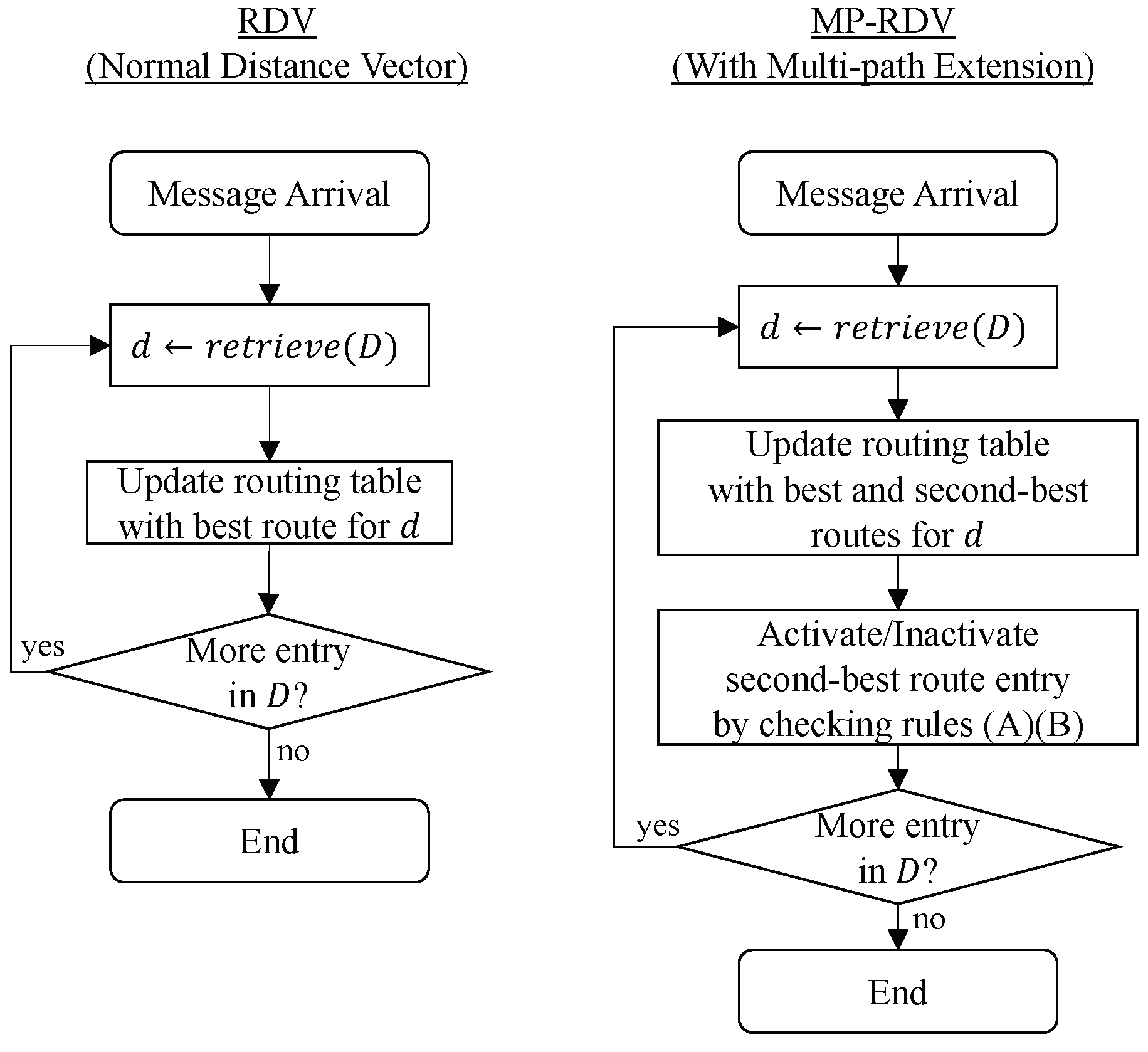
3.2. Distance-Vector Based Routing Strategy
3.3. Packet Duplication
3.4. The Routing Metric
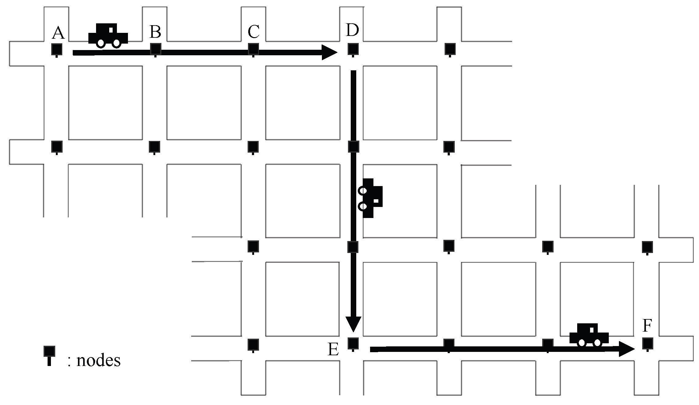
3.5. An Example
4. MP-RDV: The Proposed Scheme
4.1. Overview
4.2. Selection of Multiple Paths
- (A)
- The distance in carry of the secondary path is the same as or less than the primary path.
- (B)
- The previous-hop node of the secondary relay is different from that of the primary relay.
4.3. Extending APD for Multiple Paths
4.4. Designing Delay Metrics for MP-RDV
5. Evaluation
5.1. Methods
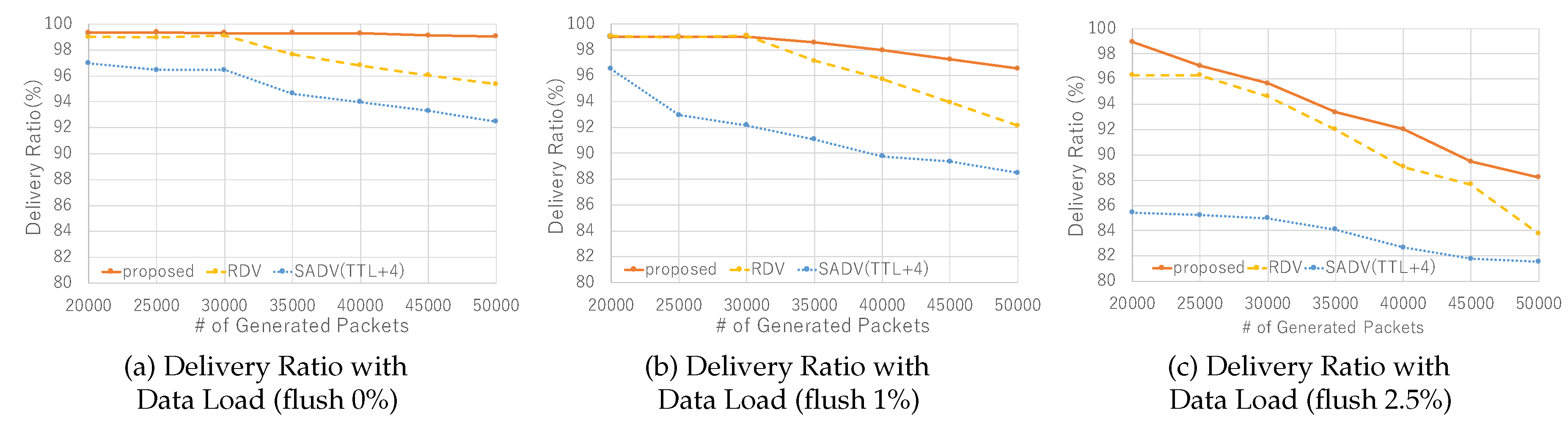
5.2. Results
5.3. Evaluating Delay Metrics
6. Conclusions
Author Contributions
Conflicts of Interest
References
- Vahdat, A.; Becker, D. Epidemic Routing for Partially Connected Ad Hoc Networks; Duke University Tech Report CS-2000-06; Duke University: Duhram, NC, USA, 2000. [Google Scholar]
- Yoo, J.; Choi, S.; Kim, C.K. The capacity of epidemic routing in vehicular networks. IEEE Commun. Lett. 2009, 13, 459–461. [Google Scholar]
- Spyropoulos, T.; Psounis, K.; Raghavendra, C.S. Spray and Wait: An Efficient Routing Scheme for Intermittently Connected Mobile Networks. In Proceedings of the ACM SIGCOMM Workshop on Delay Tolerant Networks ’05, Philadelphia, PA, USA, 26 August 2005; pp. 252–259. [Google Scholar]
- Lochert, C.; Mauve, M.; Fusler, H.; Hartenstein, H. Gergraphic Routing in City Scenarios. ACM Sigmob. Mob. Comput. Commun. Rev. 2005, 9, 69–72. [Google Scholar] [CrossRef]
- Lee, K.; Haerri, J.; Lee, U.; Gerla, M. Enhanced Perimeter Routing for Geographic Forwarding protocols in Urban Vehicular Scenarios. In Proceedings of the IEEE Globecom Workshops, Washington, DC, USA, 26–30 November 2007; pp. 1–10. [Google Scholar]
- Lochert, C.; Hartenstein, H.; Tian, J.; Fussler, H.; Hermann, D.; Mauve, M. A Routing Strategy for Vehicular Ad Hoc Networks in City Environment. In Proceedings of the IEEE Intelligent Vehicles Symposium, Columbus, OH, USA, 9–11 June 2003; pp. 156–161. [Google Scholar]
- Seet, B.C.; Liu, G.; Lee, B.S.; Foh, C.H.; Lee, K.J.; Lee, K.K. A-STAR: A Mobile Ad Hoc Routing Strategy for Metropolis Vehicular Communications. In Networking 2004; Springer: Berlin/Heidelberg, Germany, 2004; Volume 3042, pp. 989–999. [Google Scholar]
- Zhao, J.; Cao, G. VADD: Vehicle-Assisted Data Delivery in Vehicular Ad Hoc Networks. IEEE Trans. Veh. Technol. 2008, 57, 1910–1922. [Google Scholar] [CrossRef]
- Wu, H.; Fujimoto, R.; Guensler, R.; Hunter, M. MDDV: A Mobility-centric Data Dissemination Algorithm for Vehicluar Networks. In Proceedings of the VANET’04, Philadelphia, PA, USA, 1 October 2004; pp. 47–56. [Google Scholar]
- Jerbi, M.; Senouci, S.M.; Meraihi, R.; Ghamri-Doudane, Y. An improved Vehicular Ad Hoc Routing Protocol for City Environments. In Proceedings of the IEEE Internetional Conference on Communication (ICC), Glasgow, UK, 24–28 June 2007; pp. 3972–3979. [Google Scholar]
- Zhang, X.M.; Chen, K.H.; Cao, X.L.; Sung, D.K. A Street-centric Routing Protocol Based on Micro Topology in Vehicular Ad hoc Networks. IEEE Trans. Veh. Technol. 2016, 65, 5680–5694. [Google Scholar] [CrossRef]
- Ding, Y.; Xiao, L. SADV: Static-Node-Assisted Adaptive Data Dissemination in Vehicular Networks. IEEE Trans. Veh. Technol. 2010, 59, 2445–2455. [Google Scholar] [CrossRef]
- Yoshihiro, T.; Araki, D.; Sakaguchi, H.; Shibata, N. Providing Reliable Communications over Static-node-assisted Vehicular Networks Using Distance-vector Routing. Mob. Netw. Appl. 2018, 23, 1376–1393. [Google Scholar] [CrossRef]
- Araki, D.; Yoshihiro, T. A Multi-path Extension to RDV Routing Scheme for Static-node-Assisted Vehicular Networks. In Proceedings of the IEEE 32nd International Conference on Advanced Information Networking and Applications (AINA2018), Krakow, Poland, 16–18 May 2018. [Google Scholar]
- Karagiannis, G.; Altintas, O.; Ekici, E.; Heijenk, G.; Jarupan, B.; Lin, K.; Weil, T. Vehicular Networking: A Survey and Tutorial on Requirements, Architectures, Challenges, Standards and Solutions. IEEE Commun. Surv. Tutor. 2011, 13, 584–616. [Google Scholar] [CrossRef]
- Electronic Road Pricing. Available online: https://en.wikipedia.org/wiki/Electronic_Road_Pricing (accessed on 28 February 2019).
- Fujimoto, A.; Sakai, K.; Hamada, M.O.S.; Handa, S.; Matsumoto, M.; Takahashi, K. Toward Realization of SMARTWAY in Japan. In Proceedings of the 15th World Congress on Intelligent Transportation Systems (ITSWC’08), New York, NY, USA, 16–20 November 2008. [Google Scholar]
- Jeong, J.; Guo, S.; Gu, Y.; He, T.; Du, D.H.C. Trajectory-Based Statistical Forwarding for Multihop Infrastructure-to-Vehicle Data Delivery. IEEE Trans. Mob. Comput. 2012, 11, 1523–1537. [Google Scholar] [CrossRef]
- Skordylis, A.; Trigoni, N. Delay-bounded Routing in Vehicular Ad hoc Networks. In Proceedings of the MobiHoc’08, Hong Kong, China, 26–30 May 2008; pp. 341–350. [Google Scholar]
- Jarupan, B.; Ekici, E. PROMPT: A Cross-layer Position-based Communication Protocol for Delay-aware Vehicular Access Networks. Ad Hoc Netw. 2010, 8, 489–505. [Google Scholar] [CrossRef]
- Wu, Y.; Zhu, Y.; Li, B. Infrastructure-assisted Routing in Vehicular Networks. In Proceedings of the IEEE Infocom’12, Orlando, FL, USA, 25–30 March 2012. [Google Scholar]
- O’Driscoll, A.; Pesch, D. Hybrid geo-routing in urban vehicular networks. In Proceedings of the 2013 IEEE Vehicular Networking Conference, Boston, MA, USA, 16–18 December 2013; pp. 63–70. [Google Scholar]
- Li, P.; Huang, C.; Liu, Q. Delay Bounded Roadside Unit Placement in Vehicular Ad Hoc Networks. Int. J. Distrib. Sens. Netw. 2015, 2015, 1–14. [Google Scholar] [CrossRef]
- Xu, L.; Huang, C.; Wang, J.; Zhu, J.; Zhang, L. An Efficient Traffic Geographic Static-node-assisted Routing in VANET. J. Netw. 2014, 9, 1096–1102. [Google Scholar] [CrossRef]
- Li, G.; Boukhatem, L.; Wu, J. Adaptive Quality-of-Service-Based Routing for Vehicular Ad Hoc Networks With Ant Colony Optimization. IEEE Trans. Veh. Technol. 2017, 66, 3249–3264. [Google Scholar] [CrossRef]
- Goudarzi, F.; Asgari, H.; Al-Raweshidy, H.S. Traffic-Aware VANET Routing for City Environments—A Protocol Based on Ant Colony Optimization. IEEE Syst. J. 2019, 13, 571–581. [Google Scholar] [CrossRef]
- Celes, C.; Boukerche, A.; Braga, R.B.; Ramos, H.S.; Andrade, R.M.C.; Loureiro, A.A.F. Exploiting Deily Trajectories for Efficient Routing in Vehicular Ad Hoc Networks. In Proceedings of the International Conference on Communications (ICC2018), Kansas City, MO, USA, 20–24 May 2018. [Google Scholar]
- Open Street Map. Available online: https://www.openstreetmap.org/ (accessed on 28 February 2019).
- Behrisch, M.; Bieker, L.; Erdmann, J.; Krajzewicz, D. SUMO—Simulation of Urban MObility: An Overview. In Proceedings of the SIMUL2011, Barcelona, Spain, 23–29 October 2011; pp. 23–28. [Google Scholar]


| Variable | Value |
|---|---|
| P | Preconfigured expected delivery ratio. |
| Distance in carry for the destination. | |
| Expected delivery ratio on link l. | |
| Number of duplicated copies on link l. | |
| delivery ratio of link l estimated by SVS. |
| Dest. | Next,-Relay | Prev. | Dist. | Del. Ratio | Metric |
|---|---|---|---|---|---|
| ⋮ | ⋮ | ⋮ | ⋮ | ⋮ | ⋮ |
| 2 | |||||
| ⋮ | ⋮ | ⋮ | ⋮ | ⋮ | ⋮ |
| Dest. | Next,-Relay | Prev. | Dist. | Del. Ratio | Metric |
|---|---|---|---|---|---|
| ⋮ | ⋮ | ⋮ | ⋮ | ⋮ | ⋮ |
| 1 | |||||
| ⋮ | ⋮ | ⋮ | ⋮ | ⋮ | ⋮ |
© 2019 by the authors. Licensee MDPI, Basel, Switzerland. This article is an open access article distributed under the terms and conditions of the Creative Commons Attribution (CC BY) license (http://creativecommons.org/licenses/by/4.0/).
Share and Cite
Araki, D.; Yoshihiro, T. A Distance-Vector-Based Multi-Path Routing Scheme for Static-Node-Assisted Vehicular Networks. Sensors 2019, 19, 2688. https://doi.org/10.3390/s19122688
Araki D, Yoshihiro T. A Distance-Vector-Based Multi-Path Routing Scheme for Static-Node-Assisted Vehicular Networks. Sensors. 2019; 19(12):2688. https://doi.org/10.3390/s19122688
Chicago/Turabian StyleAraki, Daichi, and Takuya Yoshihiro. 2019. "A Distance-Vector-Based Multi-Path Routing Scheme for Static-Node-Assisted Vehicular Networks" Sensors 19, no. 12: 2688. https://doi.org/10.3390/s19122688
APA StyleAraki, D., & Yoshihiro, T. (2019). A Distance-Vector-Based Multi-Path Routing Scheme for Static-Node-Assisted Vehicular Networks. Sensors, 19(12), 2688. https://doi.org/10.3390/s19122688