Estimation of Interference Arrival Direction Based on a Novel Space-Time Conversion MUSIC Algorithm for GNSS Receivers

Abstract
1. Introduction
2. Signal Model
3. STC-MUSIC Algorithm
3.1. Principle and Signal Processing Process
3.2. Variable Step Size Peak Search
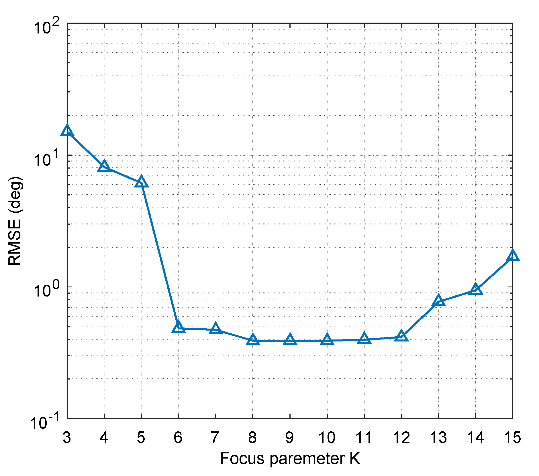
3.3. Direction-finding Focusing Parameter
3.4. Delay Units
4. Simulation Results and Analysis
4.1. Simulation of Data Block Length
4.2. Analysis of the Optimal Focusing Parameter
4.3. Performance Verification of the STC-MUSIC Algorithm
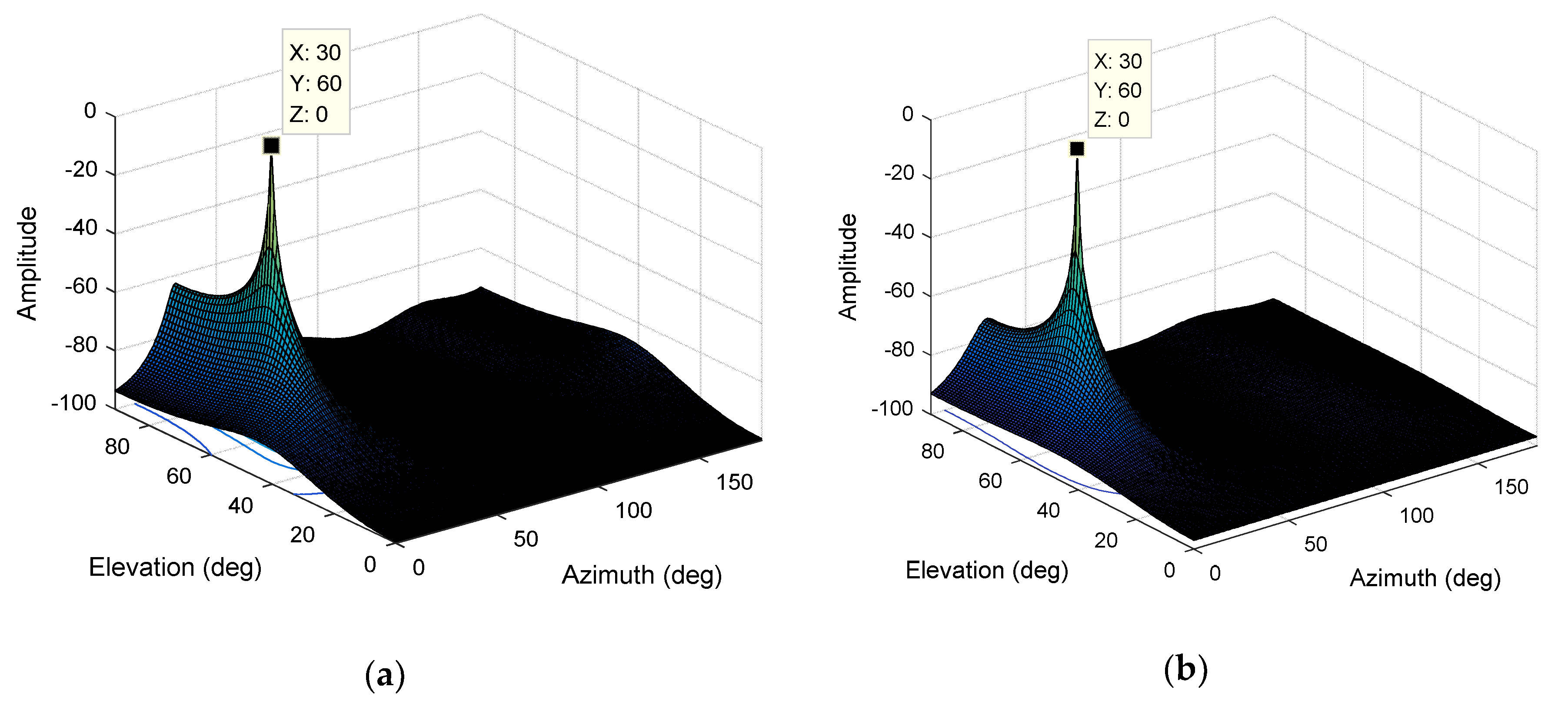
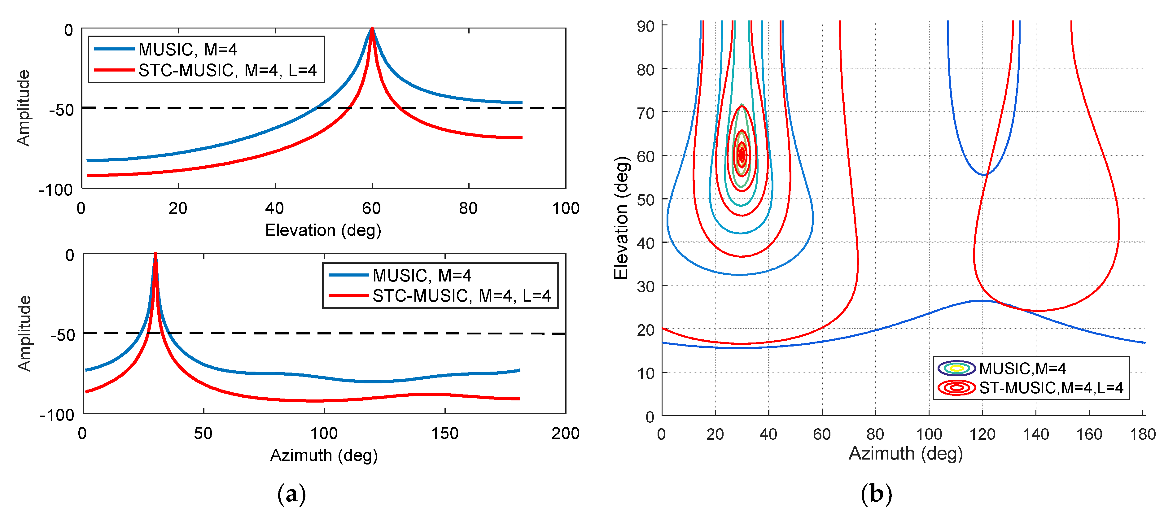
4.3.1. Single Interference Scenario
4.3.2. Multiple Interference Scenario
4.4. Evaluation of DOA Estimation Error
4.5. Test based on Actual Signal
5. Conclusions
Author Contributions
Funding
Acknowledgments
Conflicts of Interest
References
- Cetin, E.; Thompson, R.; Dempster, A.G. Passive interference localization within the GNSS environmental monitoring system (GEMS): TDOA aspects. GPS Solut. 2014, 18, 483–495. [Google Scholar] [CrossRef]
- Pal, P.; Vaidyanathan, P.P. Nested Arrays: A Novel Approach to Array Processing with Enhanced Degrees of Freedom. IEEE Trans. Signal Proc. 2010, 58, 4167–4181. [Google Scholar] [CrossRef]
- Liu, A.; Yang, Q.; Zhang, X.; Deng, W. Direction-of-Arrival Estimation for Coprime Array Using Compressive Sensing Based Array Interpolation. Int. J. Antennas Propag. 2017, 2017, 1–10. [Google Scholar] [CrossRef]
- Gao, F.; Nallanathan, A.; Wang, Y. Improved MUSIC Under the Coexistence of Both Circular and Noncircular Sources. IEEE Trans. Signal Proc. 2008, 56, 3033–3038. [Google Scholar] [CrossRef]
- Wang, Y.; Trinkle, M.; Ng, B.W.H. Efficient DOA estimation of noncircular signals in the presence of multipath propagation. Signal Proc. 2018, 149, 14–26. [Google Scholar] [CrossRef]
- Liu, A.; Li, F.; Li, B.; Liu, Q.; Shi, X. Spatial polarimetric time-frequency distribution based DOA estimation: Combining ESPRIT with MUSIC. EURASIP J. Wirel. Commun. Netw. 2018, 1, 51–58. [Google Scholar] [CrossRef]
- Cai, J.; Liu, W.; Zong, R.; Wu, B. Sparse array extension for non-circular signals with subspace and compressive sensing based DOA estimation methods. Signal Proc. 2018, 145, 59–67. [Google Scholar] [CrossRef]
- Fang-Ming, H.; Xian-Da, Z. An ESPRIT-like algorithm for coherent DOA estimation. IEEE Antennas Wirel. Propag. Lett. 2005, 4, 443–446. [Google Scholar] [CrossRef]
- Qi, C.; Wang, Y.; Zhang, Y.; Han, Y. Spatial difference smoothing for DOA estimation of coherent signals. IEEE Signal Proc. Lett. 2005, 12, 800–802. [Google Scholar] [CrossRef]
- Ledoit, O.; Wolf, M. A well-conditioned estimator for large-dimensional covariance matrices. J. Multivar. Anal. 2004, 88, 365–411. [Google Scholar] [CrossRef]
- Sun, F.; Wu, Q.; Lan, P.; Ding, G.; Chen, L. Real-valued DOA estimation with unknown number of sources via reweighted nuclear norm minimization. Signal Proc. 2018, 148, 48–55. [Google Scholar] [CrossRef]
- Chen, Z.; Ding, Y.; Ren, S.; Chen, Z. A Novel Noncircular MUSIC Algorithm Based on the Concept of the Difference and Sum Coarray. Sensors (Basel) 2018, 18, 344. [Google Scholar] [CrossRef] [PubMed]
- Zhou, C.; Gu, Y.; Shi, Z.; Zhang, Y.D. Off-Grid Direction-of-Arrival Estimation Using Coprime Array Interpolation. IEEE Signal Proc. Lett. 2018, 25, 1710–1714. [Google Scholar] [CrossRef]
- Zhou, C.; Gu, Y.; Fan, X.; Shi, Z.; Mao, G.; Zhang, Y.D. Direction-of-Arrival Estimation for Coprime Array via Virtual Array Interpolation. IEEE Trans. Signal Proc. 2018, 66, 5956–5971. [Google Scholar] [CrossRef]
- Wu, X.; Zhu, W.-P.; Yan, J. A Fast Gridless Covariance Matrix Reconstruction Method for One- and Two-Dimensional Direction-of-Arrival Estimation. IEEE Sens. J. 2017, 17, 4916–4927. [Google Scholar] [CrossRef]
- Li, J.; Li, D.; Jiang, D.; Zhang, X. Extended-Aperture Unitary Root MUSIC-Based DOA Estimation for Coprime Array. IEEE Commun. Lett. 2018, 22, 752–755. [Google Scholar] [CrossRef]
- Swindlehurst, A.L.; Kailath, T. A performance analysis of subspace-based methods in the presence of model errors. I. The MUSIC algorithm. IEEE Trans. Signal Proc. 1992, 40, 1758–1774. [Google Scholar] [CrossRef]
- Zhang, X.; Chen, C.; Li, J.; Xu, D. Blind DOA and polarization estimation for polarization-sensitive array using dimension reduction MUSIC. Multidimens. Syst. Signal Proc. 2012, 25, 67–82. [Google Scholar] [CrossRef]
- Borio, D.; Camoriano, L.; Lo Presti, L. Two-Pole and Multi-Pole Notch Filters: A Computationally Effective Solution for GNSS Interference Detection and Mitigation. IEEE Syst. J. 2008, 2, 38–47. [Google Scholar] [CrossRef]
- Daneshmand, S.; Jahromi, A.J.; Broumandan, A.; Lachapelle, G. GNSS space-time interference mitigation and attitude determination in the presence of interference signals. Sensors (Basel) 2015, 15, 12180–12204. [Google Scholar] [CrossRef]
- Richmond, C.D. Capon algorithm mean-squared error threshold SNR prediction and probability of resolution. IEEE Trans. Signal Proc. 2005, 53, 2748–2764. [Google Scholar] [CrossRef]
- Qian, C.; Huang, L.; So, H.C. Improved Unitary Root-MUSIC for DOA Estimation Based on Pseudo-Noise Resampling. IEEE Signal Proc. Lett. 2014, 21, 140–144. [Google Scholar] [CrossRef]
- Wu, Q.; Zheng, J.-S.; Dong, Z.-C.; Panayirci, E.; Wu, Z.-Q.; Qingnuobu, R. An Improved Adaptive Subspace Tracking Algorithm Based on Approximated Power Iteration. IEEE Access 2018, 6, 43136–43145. [Google Scholar] [CrossRef]


| Category | Parameter | Value |
|---|---|---|
| Signal parameter | Sampling frequency | 62 MHz |
| RF frequency | 1268.52 MHz | |
| Intermediate frequency | 46.52 MHz | |
| Array parameter | Number of array element | 4 |
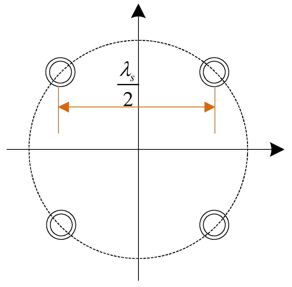
| Array type | Circular array | |
| Element spacing | Half wavelength |
| Scene 1 | Value |
|---|---|
| Number of interference | 1 |
| Type of interference | BPSK |
| Interference bandwidth | 2.046 MHz |
| JNR(Jamming-to-noise ratio) | 0 dB |
| Scene 2 | Value |
| Number of interference | 2 |
| Type of interference | a BPSK and a Gaussian |
| Interference bandwidth | 2.046 MHz |
| JNR | 0 dB |
| Parameter | Value |
|---|---|
| Number of interference | 2 |
| Type of interference | Gaussian |
| Interference bandwidth | 4 MHz |
| JNR | 20 dB |
© 2019 by the authors. Licensee MDPI, Basel, Switzerland. This article is an open access article distributed under the terms and conditions of the Creative Commons Attribution (CC BY) license (http://creativecommons.org/licenses/by/4.0/).
Share and Cite
Wang, H.; Chang, Q.; Xu, Y.; Li, X. Estimation of Interference Arrival Direction Based on a Novel Space-Time Conversion MUSIC Algorithm for GNSS Receivers. Sensors 2019, 19, 2570. https://doi.org/10.3390/s19112570
Wang H, Chang Q, Xu Y, Li X. Estimation of Interference Arrival Direction Based on a Novel Space-Time Conversion MUSIC Algorithm for GNSS Receivers. Sensors. 2019; 19(11):2570. https://doi.org/10.3390/s19112570
Chicago/Turabian StyleWang, Hao, Qing Chang, Yong Xu, and Xianxu Li. 2019. "Estimation of Interference Arrival Direction Based on a Novel Space-Time Conversion MUSIC Algorithm for GNSS Receivers" Sensors 19, no. 11: 2570. https://doi.org/10.3390/s19112570
APA StyleWang, H., Chang, Q., Xu, Y., & Li, X. (2019). Estimation of Interference Arrival Direction Based on a Novel Space-Time Conversion MUSIC Algorithm for GNSS Receivers. Sensors, 19(11), 2570. https://doi.org/10.3390/s19112570