Knowledge Preserving OSELM Model for Wi-Fi-Based Indoor Localization

 ,
,
Abstract
1. Introduction
2. Related Works
3. Background
3.1. ELM Review
| Algorithm 1: Extreme Learning Machine (ELM) Algorithm |
| Input: Output: , 2: The hidden layer output matrix, H, is calculated and defined as: is computed as represents the Moore–Penrose generalised inverse of H that results into the . C denotes the regularization parameter that is added to prevent the case of singularity. T stands for the training set’s label matrix that can be defined as where m refers to the dimension of labels that corresponds to every training sample 4: return |
3.2. OSELM Review
| Algorithm 2: ELM (OS-ELM) Algorithm |
| Inputs Output trained SLFN step 1 Boosting Phase: , where and . step 2 Sequential Learning Phase: and do based on RLS algorithm: |
3.3. FA-OSELM Review
- For every line, there is only one ‘1’; the rest of the values are all ‘0’;
- Every column has at most one ‘1’; the rest of the values are all ‘0’;
- signifies that following a change in the feature dimension, the ith dimension of the original feature vector will become the jth dimension of the new feature vector.
- Lower feature dimensions indicate that can be termed as an all-zero vector. Hence, no additional corresponding input weight is required by the newly added features;
- In cases where the feature dimension increases, if the new feature is embodied by the ith item of , a random generation of the ith item of should be carried out based on the distribution of .
4. Methodology
4.1. Generating Dynamic Scenarios of Localization
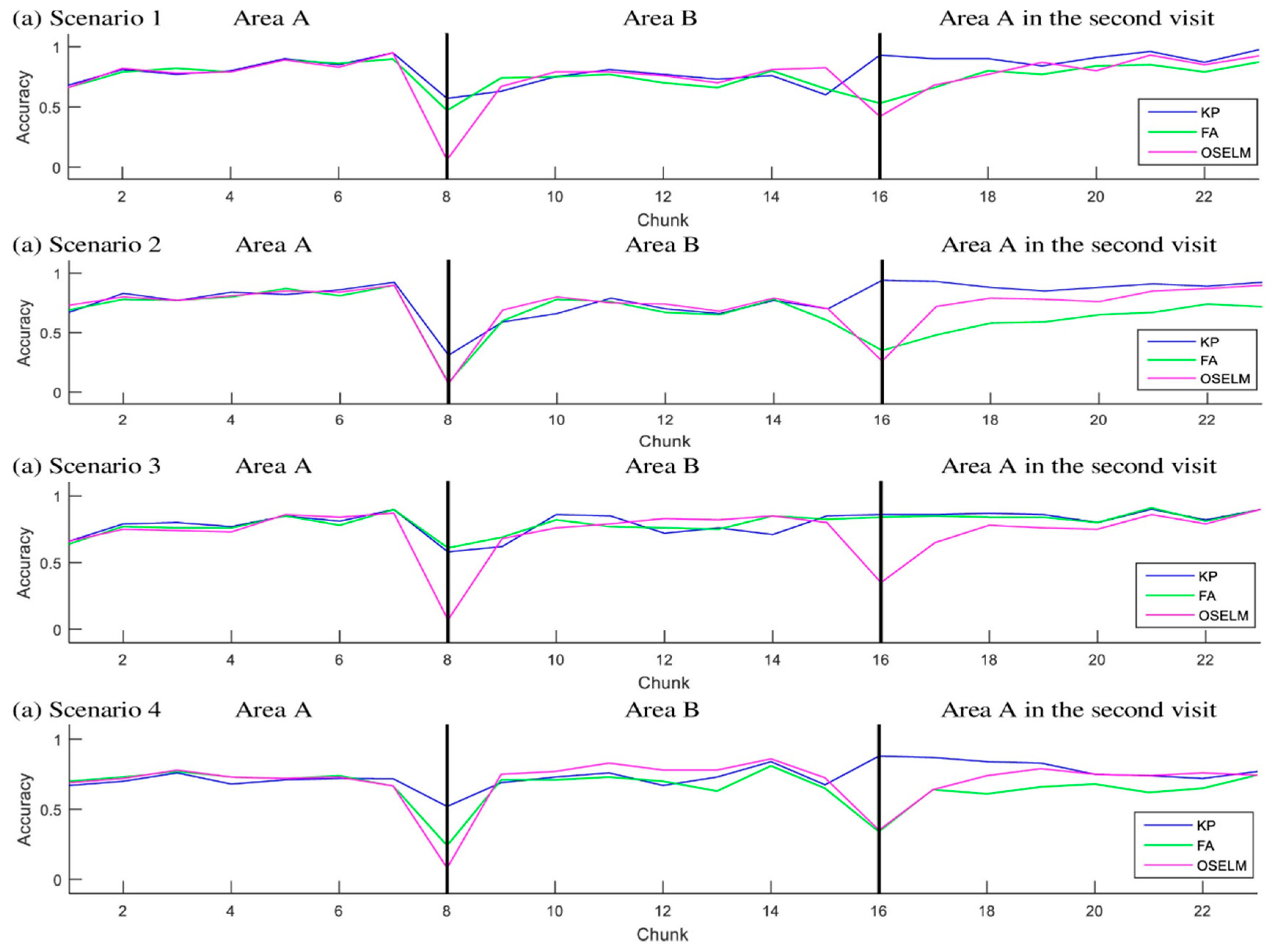
- A person moves from area A to area B. The number of APs in A () is higher than the number of features in B (). The APs in B are contained in the APs in A or . Then, the person returns to area A as represented in Figure 2a. The red line represents the trajectory from A to B, whereas the blue line presents the trajectory from B to A. All APs are in side A, such that .
- A person moves from area A to area B. The number of APs in A () is higher than or equal to the number of features in B ). The APs in B are not contained in the APs in A or . Then, the person returns to area A as represented in Figure 2b. Similar to the previous scenario, the red line represents the trajectory from A to B, whereas the blue line represents the trajectory from B to A. The APs are distributed on sides A and B with higher density in side A than in side B, such that and .
- A person moves from area A to area B. The number of APs in A ) is lower than the number of features in B . The APs in B are contained in the APs in A or . Then, the person returns to area A as represented in Figure 2c. The APs are distributed on side B only. Thus, the rule of is applied.
- A person moves from area A to area B. The number of APs in A () is lower than or equal to the number of features in B (). The APs in B are not contained in the APs in A or . Then, the person returns to area A as represented in Figure 2d. The APs are distributed on both sides with higher density in side B than in side A. Table 2 summarizes these scenarios.
4.2. Neural Network Structure for Knowledge-Preserving Neural Network and Feature Coding
- The number of inputs is variable which equals to the number of APs that are sensed in the area. The number of hidden neurons is which is determined with the regularization parameter by using the characterization model (which is built on the basis of the training data).
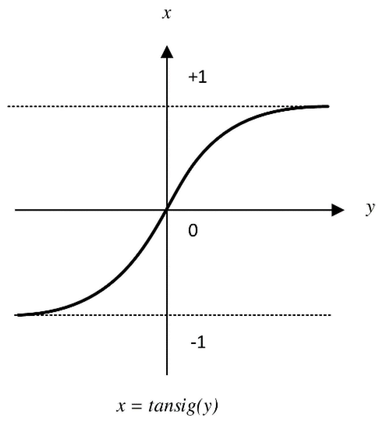
- The activation function is tansig
4.3. General Algorithmic Procedure
4.4. Computational Analysis
5. Experimental Results
5.1. Datasets Description
5.2. Characterization Model
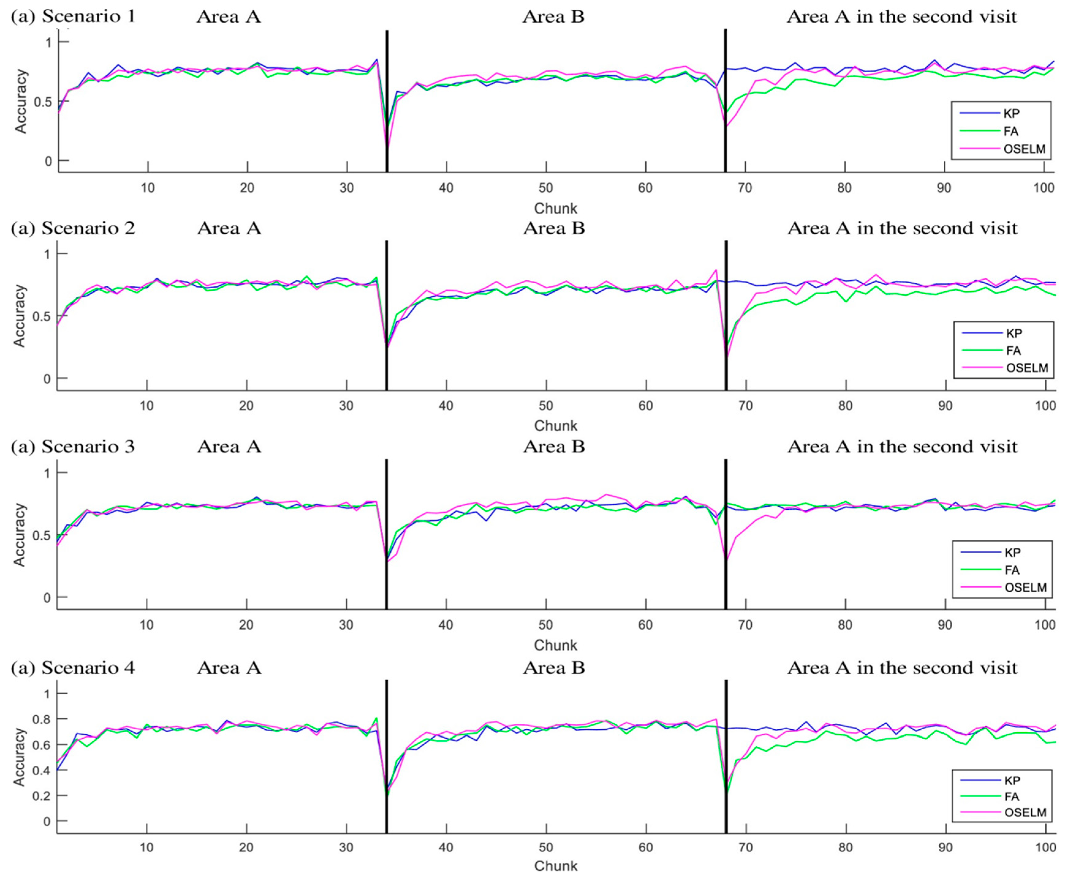
5.3. Areas Based Scenarios
5.3.1. Accuracy
5.3.2. Statistical Based Comparison
5.3.3. Standard Deviation
5.4. Trajectory Based Scenarios
6. Summary and Conclusions
Author Contributions
Funding
Conflicts of Interest
References
- Wan, J.; Zou, C.; Ullah, S.; Lai, C.; Zhou, M.; Wang, X. Cloud-Enabled Wireless Body Area Networks for Pervasive Healthcare. IEEE Netw. 2013, 27, 56–61. [Google Scholar] [CrossRef]
- Ali, M.U.; Hur, S.; Park, Y. LOCALI: Calibration-Free Systematic Localization Approach for Indoor Positioning. Sensors 2017, 17, 1213. [Google Scholar] [CrossRef]
- Umanets, A.; Ferreira, A.; Leite, N. GuideMe—A Tourist Guide with a Recommender System and Social Interaction. Procedia Technol. 2014, 17, 407–414. [Google Scholar] [CrossRef]
- Wang, S.; Fidler, S.; Urtasun, R. Lost Shopping! Monocular Localization in Large Indoor Spaces. In Proceedings of the IEEE International Conference on Computer Vision (ICCV), Santiago, Chile, 7–13 December 2015; pp. 2695–2703. [Google Scholar]
- Xu, H.; Ding, Y.; Li, P.; Wang, R.; Li, Y. An RFID Indoor Positioning Algorithm Based on Bayesian Probability and K-Nearest Neighbor. Sensors 2017, 17, 1806. [Google Scholar] [CrossRef] [PubMed]
- Azizyan, M.; Constandache, I.; Choudhury, R.R. SurroundSense: Mobile Phone Localization Via Ambience Fingerprinting. In Proceedings of the 15th Annual International Conference on Mobile Computing and Networking, Beijing, China, 21–23 June 2009; pp. 261–272. [Google Scholar]
- Chen, C.-S. Artificial Neural Network for Location Estimation in Wireless Communication Systems. Sensors 2012, 12, 2798–2817. [Google Scholar] [CrossRef]
- Ibrahim, M.; Youssef, M. A Hidden Markov Model for Localization Using Low-End GSM Cell Phones. In Proceedings of the IEEE International Conference on Communications (ICC), Kyoto, Japan, 5–9 June 2011; pp. 1–5. [Google Scholar]
- Sánchez-Rodríguez, D.; Hernández-Morera, P.; Quinteiro, J.M.; Alonso-González, I. A Low Complexity System Based on Multiple Weighted Decision Trees for Indoor Localization. Sensors 2015, 15, 14809–14829. [Google Scholar] [CrossRef]
- Jiang, X.; Liu, J.; Chen, Y.; Liu, D.; Gu, Y.; Chen, Z. Feature Adaptive Online Sequential Extreme Learning Machine for Lifelong Indoor Localization. Neural Comput. Appl. 2016, 27, 215–225. [Google Scholar] [CrossRef]
- Zou, H.; Lu, X.; Jiang, H.; Xie, L. A Fast and Precise Indoor Localization Algorithm Based on an Online Sequential Extreme Learning Machine. Sensors 2015, 15, 1804–1824. [Google Scholar] [CrossRef]
- Huang, G.B.; Zhu, Q.Y.; Siew, C.K. Extreme Learning Machine: A New Learning Scheme of Feedforward Neural Networks. In Proceedings of the IEEE International Joint Conference on Neural Networks (IEEE Cat. No.04CH37541), Budapest, Hungary, 25–29 July 2004; pp. 985–990. [Google Scholar]
- Salamah, A.H.; Tamazin, M.; Sharkas, M.A.; Khedr, M. An Enhanced WiFi Indoor Localization System Based on Machine Learning. In Proceedings of the Indoor Positioning and Indoor Navigation (IPIN), Alcala de Henares, Spain, 4–7 October 2016; pp. 1–8. [Google Scholar]
- Huang, G.B.; Chen, L.; Siew, C.K. Universal Approximation Using Incremental Constructive Feedforward Networks with Random Hidden Nodes. IEEE Trans. Neural Netw. 2006, 17, 879–892. [Google Scholar] [CrossRef]
- Liang, N.Y.; Huang, G.B.; Saratchandran, P.; Sundararajan, N. A Fast and Accurate Online Sequential Learning Algorithm for Feedforward Networks. IEEE Trans. Neural Netw. 2006, 17, 1411–1423. [Google Scholar] [CrossRef] [PubMed]
- Zhang, L.; Zhang, D. Robust Visual Knowledge Transfer Via Extreme Learning Machine Based Domain Adaptation. IEEE Trans. Image Process. 2016, 25, 4959–4973. [Google Scholar] [CrossRef]
- Zhang, L.; Zhang, D. Domain Adaptation Extreme Learning Machines for Drift Compensation in E-Nose Systems. IEEE Trans. Instrum. Meas. 2015, 64, 1790–1801. [Google Scholar] [CrossRef]
- Uzair, M.; Mian, A. Blind Domain Adaptation with Augmented Extreme Learning Machine Features. IEEE Trans. Cybern. 2017, 47, 651–660. [Google Scholar] [CrossRef] [PubMed]
- Jain, V.; Learned-Miller, E. Online Domain Adaptation of a Pre-Trained Cascade of Classifiers. In Proceedings of the IEEE Conference on Computer Vision and Pattern Recognition (CVPR), Washington, DC, USA, 20–25 June 2011; pp. 577–584. [Google Scholar]
- Lu, X.; Long, Y.; Zou, H.; Yu, C.; Xie, L. Robust Extreme Learning Machine for Regression Problems with its Application to WIFI Based Indoor Positioning System. In Proceedings of the IEEE International Workshop on Machine Learning for Signal Processing (MLSP), Reims, France, 21–24 September 2014; pp. 1–6. [Google Scholar]
- Lu, X.; Zou, H.; Zhou, H.; Xie, L.; Huang, G. Robust Extreme Learning Machine with Its Application to Indoor Positioning. IEEE Trans. Cybern. 2016, 46, 194–205. [Google Scholar] [CrossRef] [PubMed]
- Zhang, M.; Wen, Y.; Chen, J.; Yang, X.; Gao, R.; Zhao, H. Pedestrian Dead-Reckoning Indoor Localization Based on Os-Elm. IEEE Access 2018, 6, 6116–6129. [Google Scholar] [CrossRef]
- AL-Khaleefa, A.S.; Ahmad, M.R.; Isa, A.A.M.; AL-Saffar, A.; Esa, M.R.M.; Malik, R.F. MFA-OSELM Algorithm for WiFi-Based Indoor Positioning System. Information 2019, 10, 146. [Google Scholar] [CrossRef]
- AL-Khaleefa, A.S.; Ahmad, M.R.; Isa, A.A.M.; Esa, M.R.M.; AL-Saffar, A.; Hassan, M.H. Feature Adaptive and Cyclic Dynamic Learning Based on Infinite Term Memory Extreme Learning Machine. Appl. Sci. 2019, 9, 895. [Google Scholar] [CrossRef]
- Al-Khaleefa, A.S.; Ahmad, M.R.; Md Isa, A.A.; Mohd Esa, M.R.; Al-Saffar, A.; Aljeroudi, Y. Infinite-Term Memory Classifier for Wi-Fi Localization Based on Dynamic Wi-Fi Simulator. IEEE Access 2018, 6, 54769–54785. [Google Scholar] [CrossRef]
- Huang, G.-B.; Liang, N.-Y.; Rong, H.-J.; Saratchandran, P.; Sundararajan, N. On-Line Sequential Extreme Learning Machine. Comput. Intell. 2005, 2005, 232–237. [Google Scholar]
- Liu, X.; Gao, C.; Li, P. A Comparative Analysis of Support Vector Machines and Extreme Learning Machines. Neural Netw. 2012, 33, 58–66. [Google Scholar] [CrossRef]
- Torres-Sospedra, J.; Montoliu, R.; Martínez-Usó, A.; Avariento, J.P.; Arnau, T.J.; Benedito-Bordonau, M.; Huerta, J. UJIIndoorLoc: A New Multi-Building and Multi-Floor Database for WLAN Fingerprint-Based Indoor Localization Problems. In Proceedings of the International Conference on Indoor Positioning and Indoor Navigation (IPIN), Busan, Korea, 27–30 October 2014; pp. 261–270. [Google Scholar]
- Lohan, S.E.; Torres-Sospedra, J.; Leppäkoski, H.; Richter, P.; Peng, Z.; Huerta, J. Wi-Fi Crowdsourced Fingerprinting Dataset for Indoor Positioning. Data 2017, 2, 32. [Google Scholar] [CrossRef]


| Symbol | Description | Symbol | Description |
|---|---|---|---|
| The number of input | Output matrix | ||
| The record of features | Target vectors | ||
| The target of certain record | Number of features | ||
| An index | Index | ||
| Biases | Intermediate matrix | ||
| An activation function | RLS | Recursive least square | |
| Number of neurons in the hidden layer | Weights between input hidden layer | ||
| Weights between hidden output layer | Regularization parameter |
| Scenario Name | Mobility | Number of APs Relation | APs Subset Relation |
|---|---|---|---|
| S1 | A→B→A | ||
| S2 | A→B→A | ||
| S3 | A→B→A | ||
| S4 | A→B→A |
| Input: |
| trainD: Raw training dataset of Wi-Fi fingerprint |
| testD: Raw testing dataset of Wi-Fi fingerprint |
| A, B: Two locations with common features |
| NA: Number of features in location A |
| NB: Number of features in location B |
| Output: |
| trainDataA |
| trainDataAf |
| trainDataB |
| trainDataBf |
| testDataAf |
| testDataBf |
| Start: |
| 1- Replace all 100 in trainD and testD with 0 //preprocessing |
| 2- nData = number of records in trainD |
| 3- number of RecordsA=nData/2 |
| 4- testDataA = testD |
| 5- testDataB = testD //testData is the same for location A and B |
| 6- nFeatures = number of features in dataset |
| 7- nFeatures = 1:nFeatures //create vector of features labels 1,2..nFatures |
| 8- featuresA = getRandom(features,NA) //select NA random features from features |
| 9- featuresB = getRandom(featuresA,NB) //select NB random features from featuresA because B is contained in A |
| 10- trainDataA = trainData(1:numberofRecordsA) |
| 11- trainDataB = trainData(numberofRecordsA+1:end) |
| 12- trainDataAf = generateFeaturesData(trainDataA, featuresA) |
| 13- testDataAf = generateFeaturesData(testDataA, featuresA) |
| 14- trainDataBf = GenerateFeaturesData(trainDataB, featuresB) |
| 15- testDataBf = GenerateFeaturesData(testDataB, featuresB) |
| End |
| X1 | X2 | X3 | X4 | X5 | Y |
|---|---|---|---|---|---|
| 30 | 50 | 60 | 0 | 0 | 1 |
| 35 | 45 | 55 | 0 | 0 | 1 |
| 60 | 10 | 12 | 0 | 0 | 2 |
| 55 | 14 | 11 | 0 | 0 | 2 |
| 50 | 20 | 9 | 0 | 0 | 2 |
| 0 | 0 | 70 | 30 | 25 | 3 |
| 0 | 0 | 88 | 33 | 30 | 3 |
| 0 | 0 | 40 | 70 | 60 | 4 |
| 0 | 0 | 36 | 66 | 59 | 4 |
| Inputs: |
| //chunks of data with constraint of FC to be zero when k is constant |
| //vector of labels of chunk , it is only provided after the neural |
| network makes the prediction of |
| //initial neural network |
| Outputs: |
| ACC //accuracy of prediction |
| Start: |
| 1- =Encode() //this function encode the non-active features with zeros |
| 2- OSELMTrain() |
| 3- For =1 until N |
| =Encode() |
| 5- Predict() |
| 6- ACC=calculateAccuracy() 7- OSELMTrain() |
| End |
| Parameter Name | Parameter Description | Scenario 1 | Scenario 2 | Scenario 3 | Scenario 4 |
|---|---|---|---|---|---|
| NA | Number of features in location A | 100 | 100 | 50 | 50 |
| NB | Number of features in location B | 50 | 50 | 100 | 100 |
| NCF-AB | Number of Common features between A and B | 50 | 11 | 50 | 15 |
| L | Number of hidden neurons | 750 | 750 | 750 | 750 |
| Parameter Name | Parameter Description | Scenario 1 | Scenario 2 | Scenario 3 | Scenario 4 |
|---|---|---|---|---|---|
| NA | Number of features in location A | 300 | 300 | 150 | 150 |
| NB | Number of features in location B | 150 | 150 | 300 | 300 |
| NCF-AB | Number of Common features between A and B | 150 | 99 | 150 | 80 |
| L | Number of hidden neurons | 850 | 850 | 850 | 850 |
| Scenario No. | Algorithms 1 vs. Algorithm 2 | Area A | Area B | Area A2 |
|---|---|---|---|---|
| Scenario 1 | KP-OSELM vs. OSELM | 0.280 | 0.437 | 0.086 |
| KP-OSELM vs. FA-OSELM | 0.558 | 0.530 | 0.017 | |
| Scenario 2 | KP-OSELM vs. OSELM | 0.871 | 0.906 | 0.085 |
| KP-OSELM vs. FA-OSELM | 0.383 | 0.584 | 0.001 | |
| Scenario 3 | KP-OSELM vs. OSELM | 0.190 | 0.630 | 0.063 |
| KP-OSELM vs. FA-OSELM | 0.023 | 0.466 | 0.066 | |
| Scenario 4 | KP-OSELM vs. OSELM | 0.369 | 0.864 | 0.156 |
| KP-OSELM vs. FA-OSELM | 0.288 | 0.195 | 0.016 |
| Scenario No. | Algorithms 1 vs. Algorithm 2 | Area A | Area B | Area A2 |
|---|---|---|---|---|
| Scenario 1 | KP-OSELM vs. OSELM | 0.462 | 0.004 | 0.007 |
| KP-OSELM vs. FA-OSELM | 0.000 | 0.532 | 0.000 | |
| Scenario 2 | KP-OSELM vs. OSELM | 0.650 | 0.000 | 0.069 |
| KP-OSELM vs. FA-OSELM | 0.184 | 0.198 | 0.000 | |
| Scenario 3 | KP-OSELM vs. OSELM | 0.439 | 0.000 | 0.175 |
| KP-OSELM vs. FA-OSELM | 0.540 | 0.690 | 0.006 | |
| Scenario 4 | KP-OSELM vs. OSELM | 0.084 | 0.000 | 0.068 |
| KP-OSELM vs. FA-OSELM | 0.550 | 0.316 | 0.000 |
| Dataset | Algorithm | Cycle 1 | Cycle 2 | Cycle 3 |
|---|---|---|---|---|
| Rectangle TampereU dataset | KP-OSELM | 67.81% | 92.74% | 92.74% |
| FA-OSELM | 68.94% | 72.33% | 78.28% | |
| OSELM | 8.06% | 5.74% | 7.99% | |
| Rectangle UJIndoorLoc dataset | KP-OSELM | 48.88% | 73.03% | 72.99% |
| FA-OSELM | 31.53% | 32.52% | 38.2% | |
| OSELM | 15.95% | 14.08% | 13.12% |
© 2019 by the authors. Licensee MDPI, Basel, Switzerland. This article is an open access article distributed under the terms and conditions of the Creative Commons Attribution (CC BY) license (http://creativecommons.org/licenses/by/4.0/).
Share and Cite
AL-Khaleefa, A.S.; Ahmad, M.R.; Isa, A.A.M.; Esa, M.R.M.; Aljeroudi, Y.; Jubair, M.A.; Malik, R.F. Knowledge Preserving OSELM Model for Wi-Fi-Based Indoor Localization. Sensors 2019, 19, 2397. https://doi.org/10.3390/s19102397
AL-Khaleefa AS, Ahmad MR, Isa AAM, Esa MRM, Aljeroudi Y, Jubair MA, Malik RF. Knowledge Preserving OSELM Model for Wi-Fi-Based Indoor Localization. Sensors. 2019; 19(10):2397. https://doi.org/10.3390/s19102397
Chicago/Turabian StyleAL-Khaleefa, Ahmed Salih, Mohd Riduan Ahmad, Azmi Awang Md Isa, Mona Riza Mohd Esa, Yazan Aljeroudi, Mohammed Ahmed Jubair, and Reza Firsandaya Malik. 2019. "Knowledge Preserving OSELM Model for Wi-Fi-Based Indoor Localization" Sensors 19, no. 10: 2397. https://doi.org/10.3390/s19102397
APA StyleAL-Khaleefa, A. S., Ahmad, M. R., Isa, A. A. M., Esa, M. R. M., Aljeroudi, Y., Jubair, M. A., & Malik, R. F. (2019). Knowledge Preserving OSELM Model for Wi-Fi-Based Indoor Localization. Sensors, 19(10), 2397. https://doi.org/10.3390/s19102397