Orthogonal Frequency Division Multiplexing Techniques Comparison for Underwater Optical Wireless Communication Systems


Abstract
1. Introduction
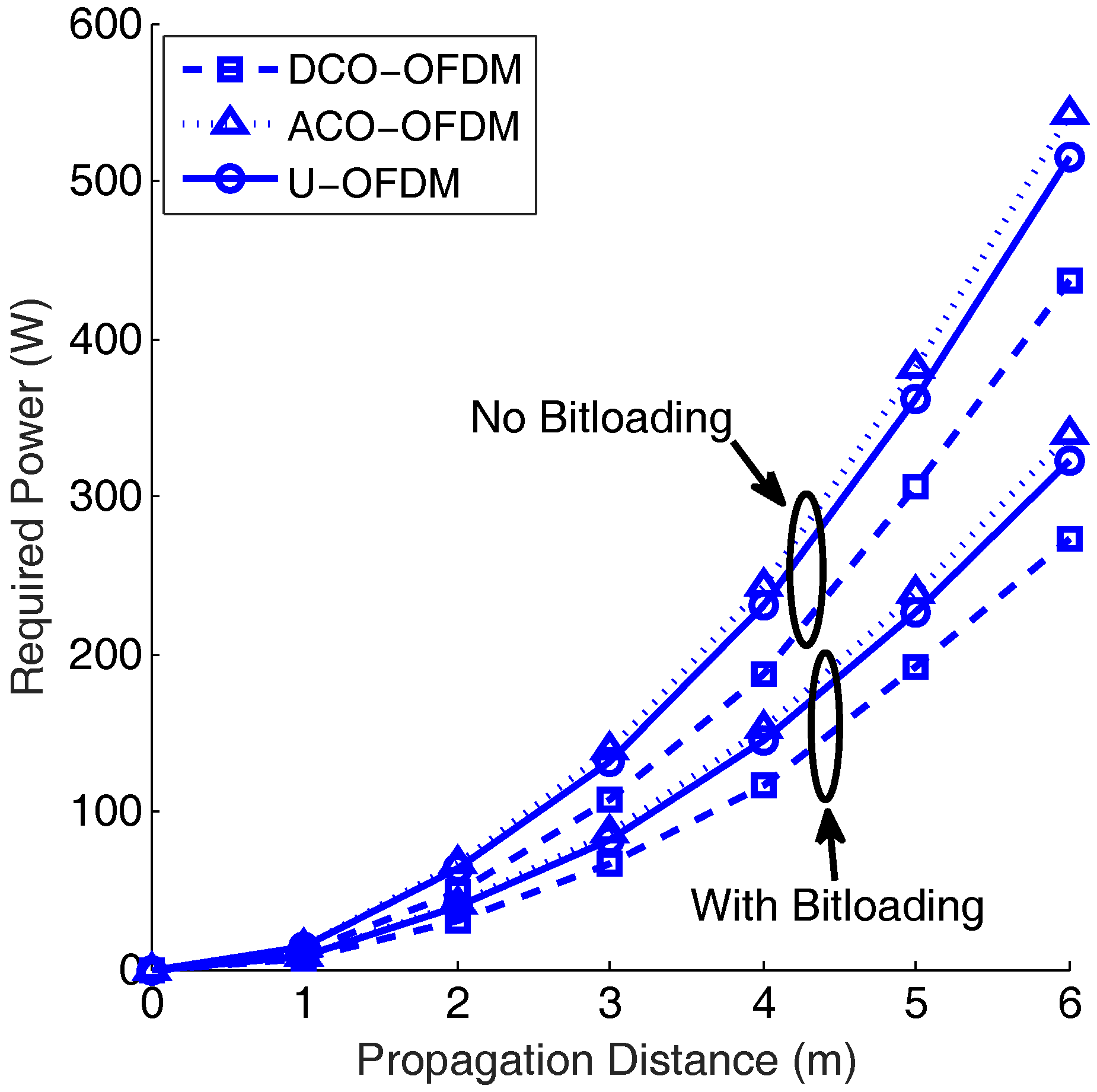
- A comparison of the state-of-the-art optical OFDM techniques for underwater optical wireless communication systems is discussed based on the propagation distance, BER, and data throughput.
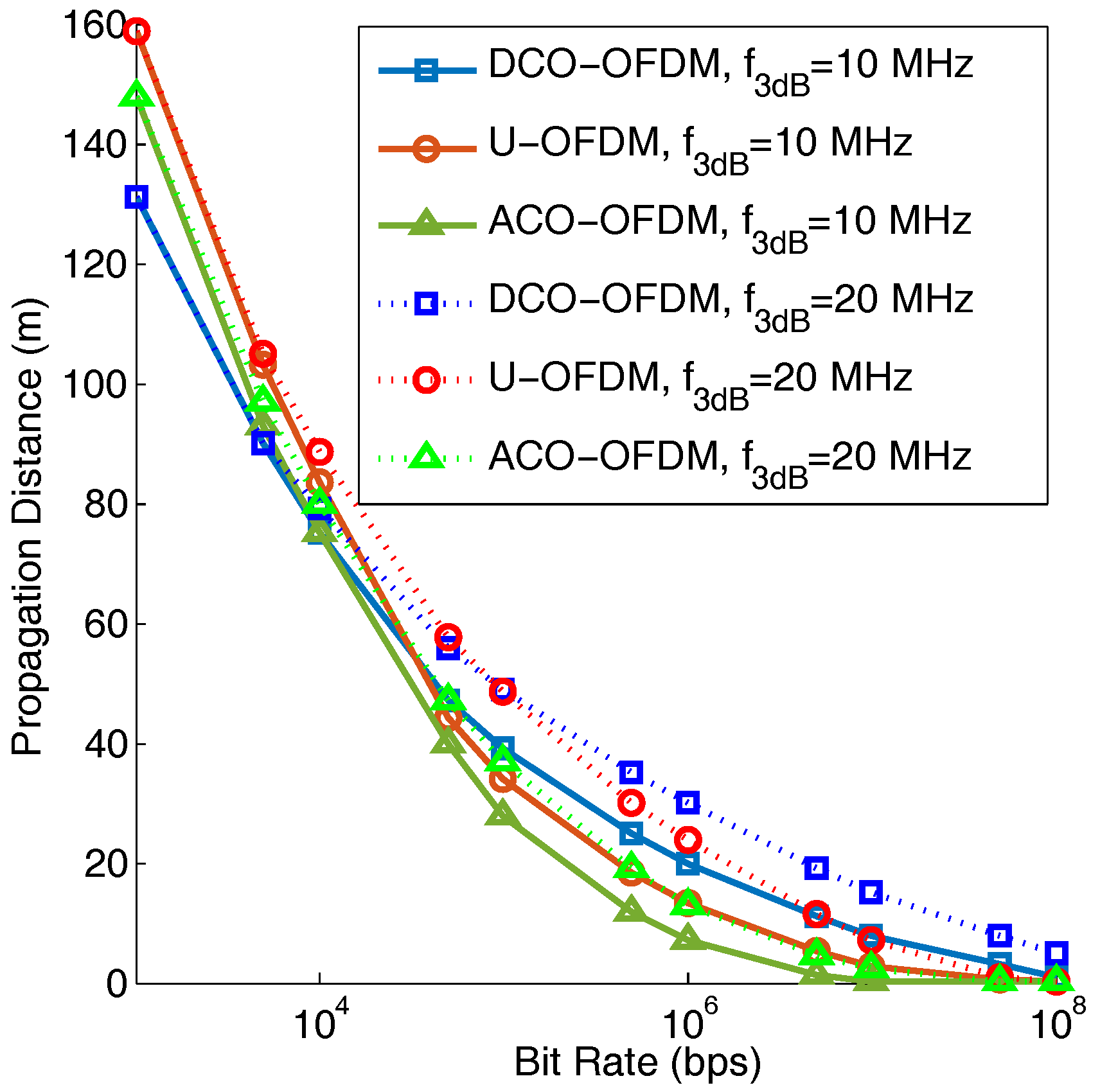
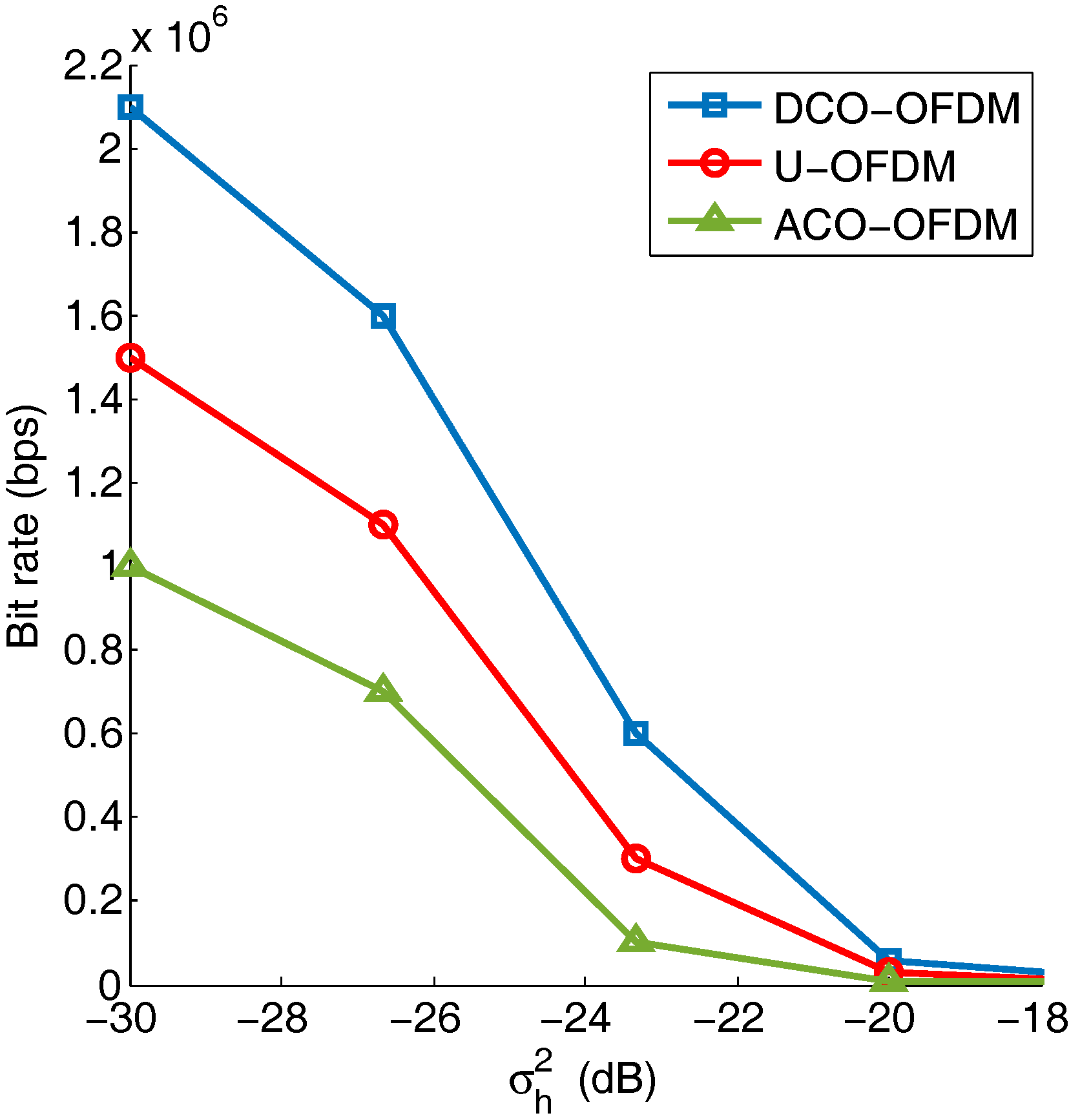
- Considering the turbulence fading underwater channel, the performances of ACO-, DCO-, and U-OFDM using the channels with different bandwidths are tested.
- For different transmitted bit rates, the achievable propagation distances of DCO-, ACO-, and U-OFDM with the band-limited channel are discussed.
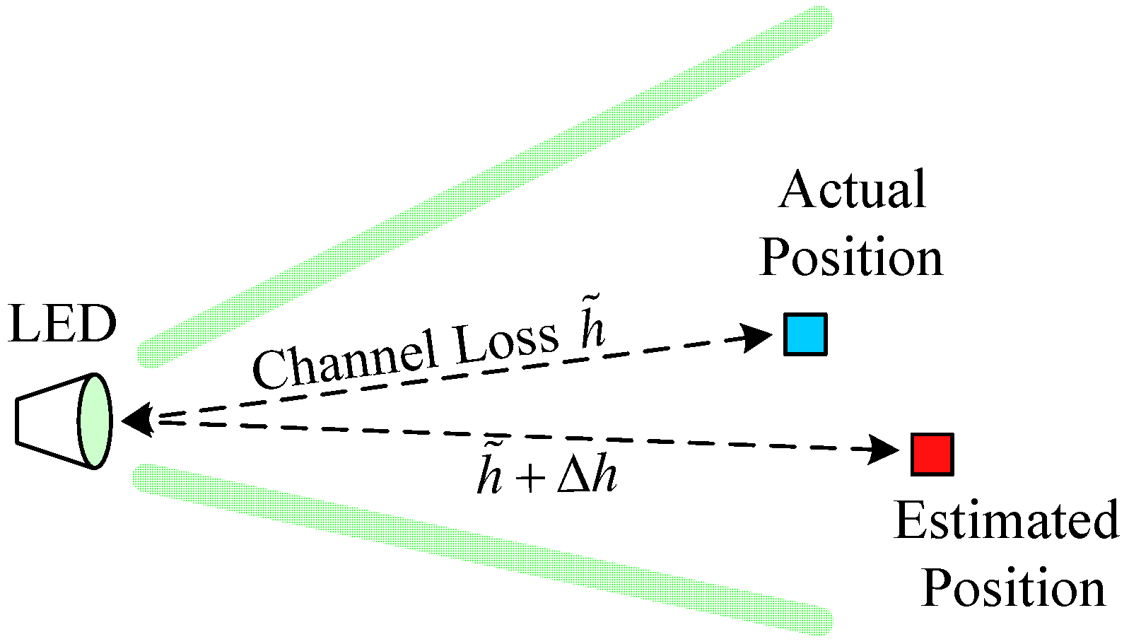
- The underwater channel uncertainty caused by the pointing error is modeled and tested.
2. Research Problem
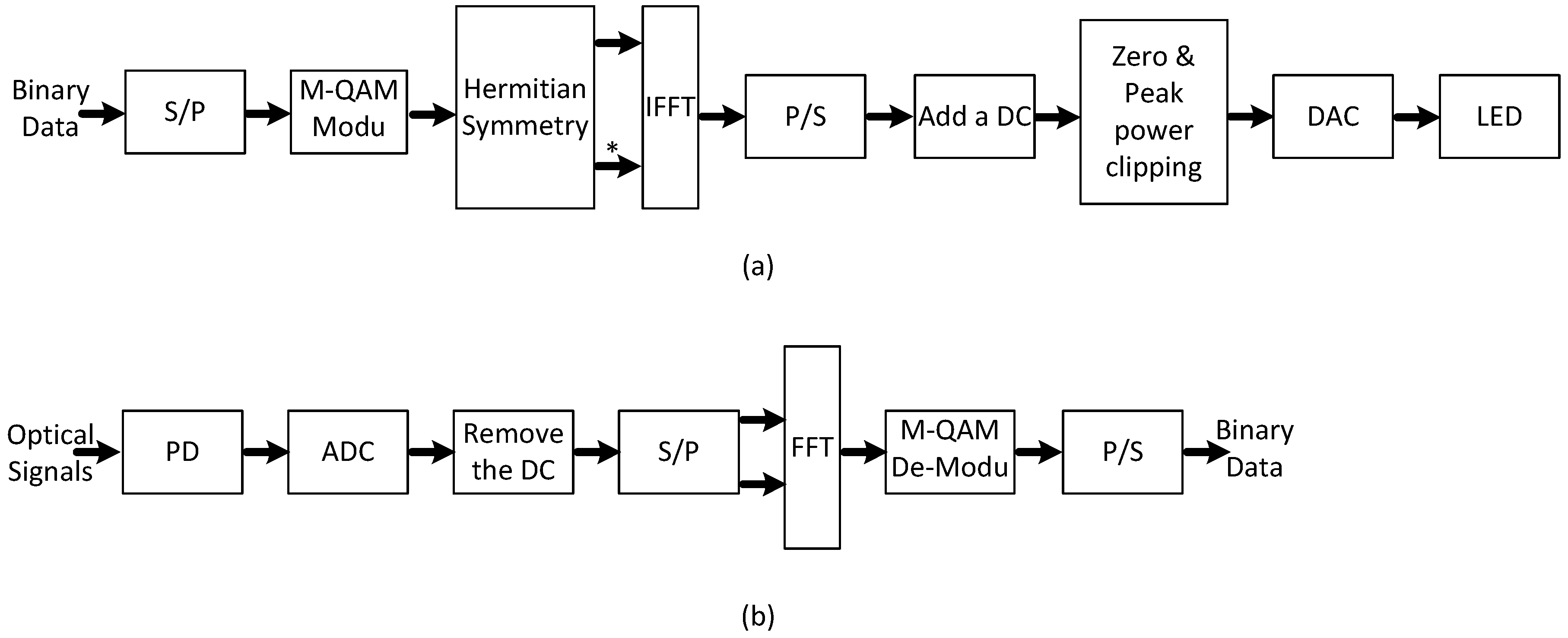
2.1. RF OFDM vs. Optical OFDM
2.2. Underwater Optical Channel Model
2.3. Channel Estimation Error and Pointing Error
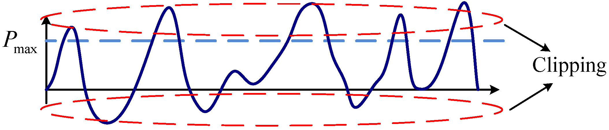
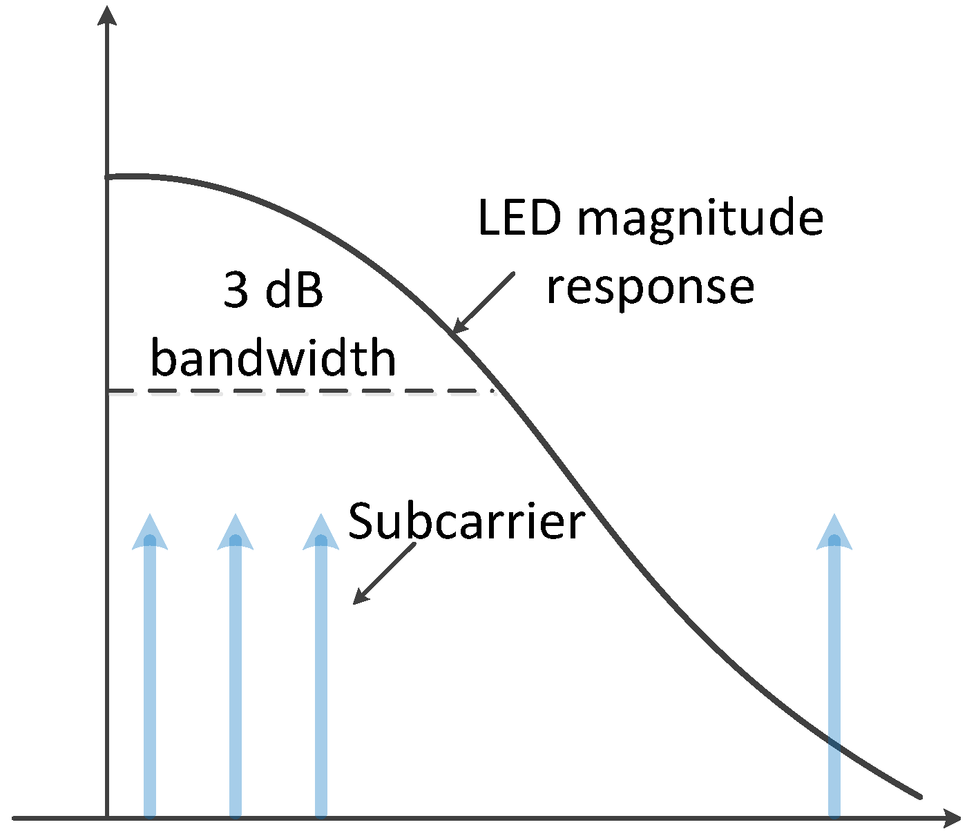
2.4. Power and Bandwidth Constraints of LEDs
3. Analysis of Optical OFDM for Underwater Communications
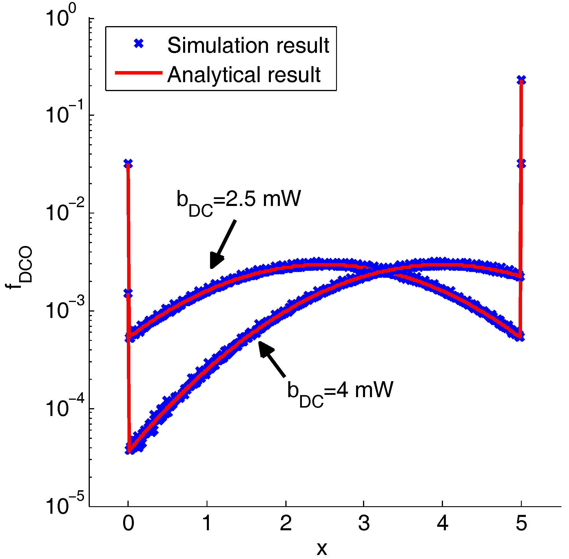
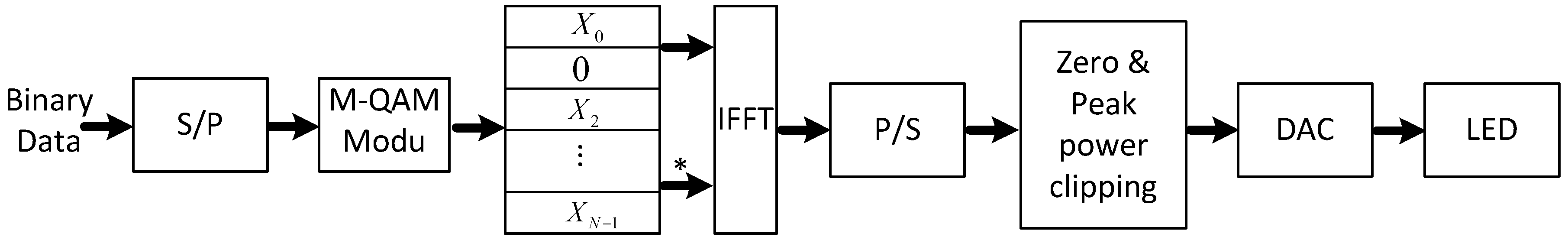
3.1. DCO-OFDM
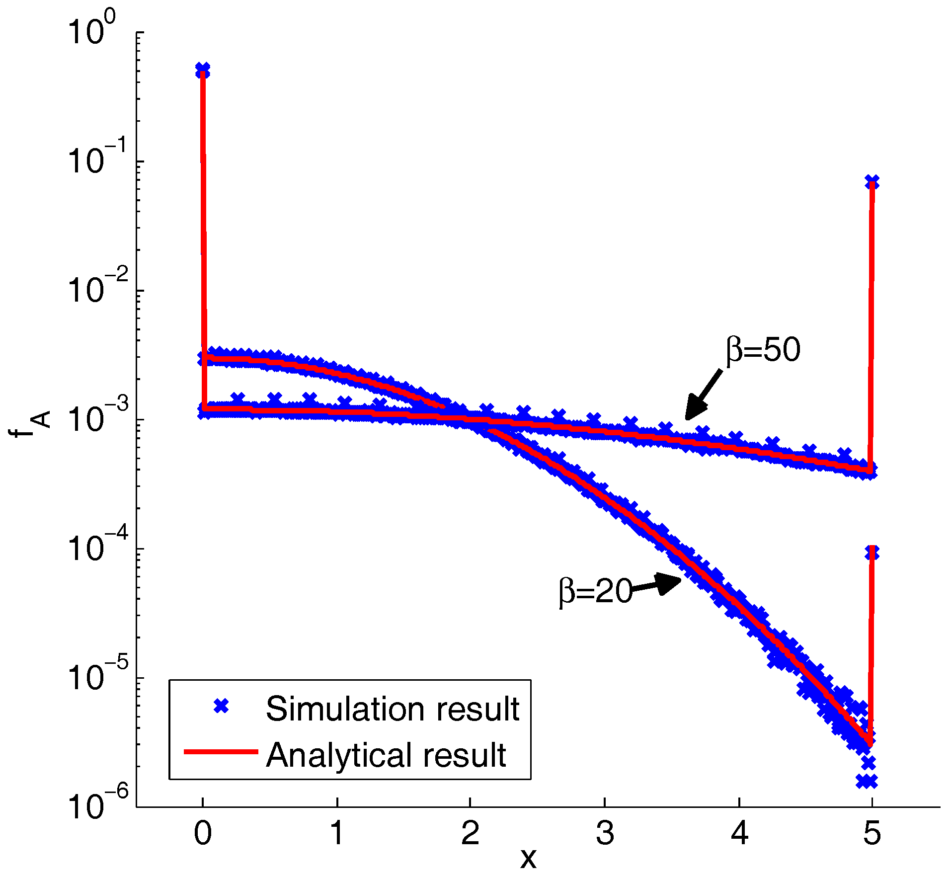
3.2. ACO-OFDM
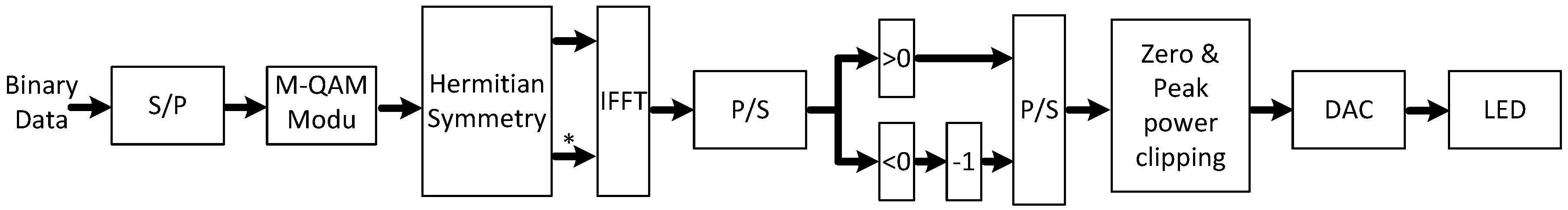
3.3. U-OFDM
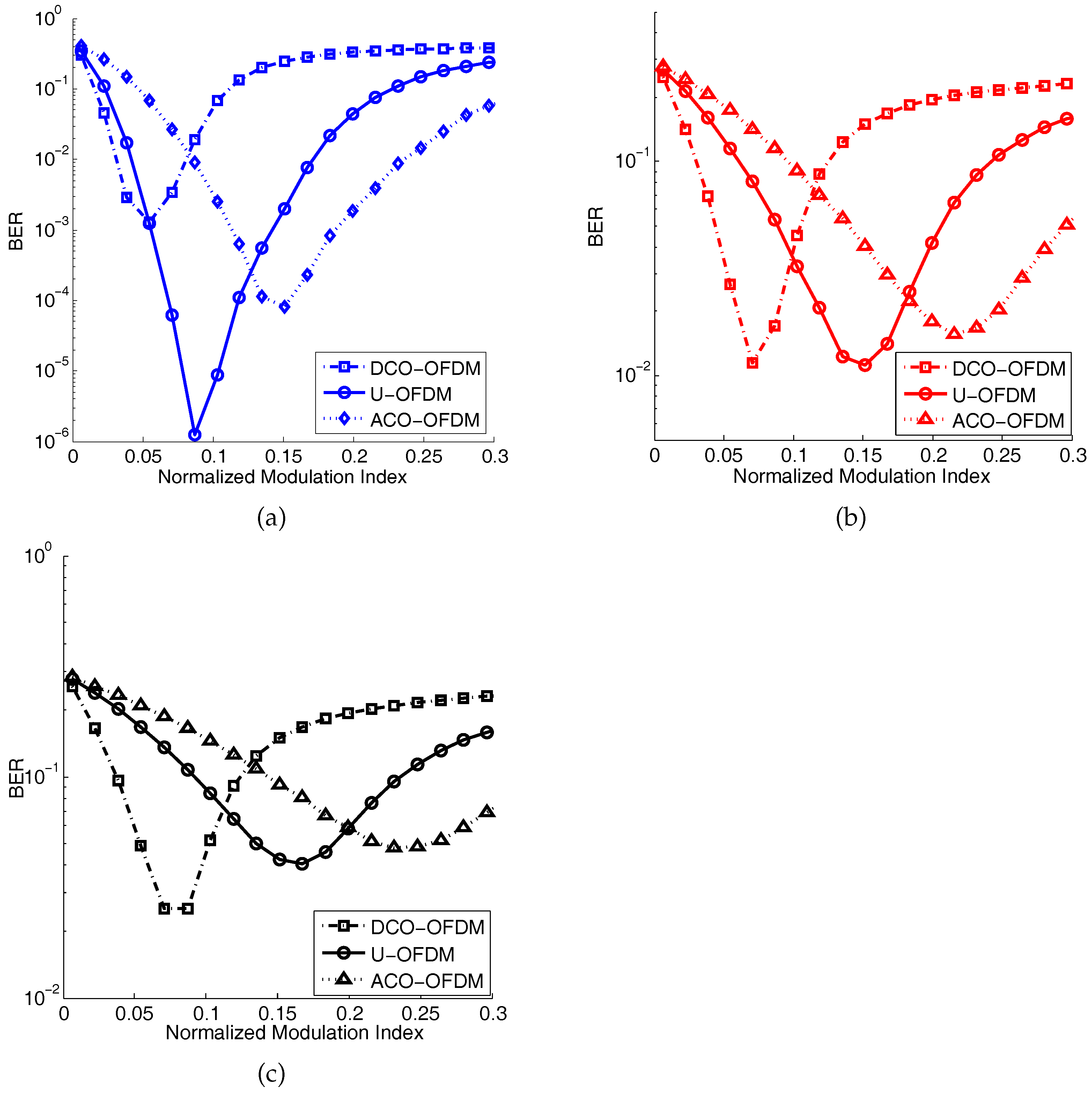
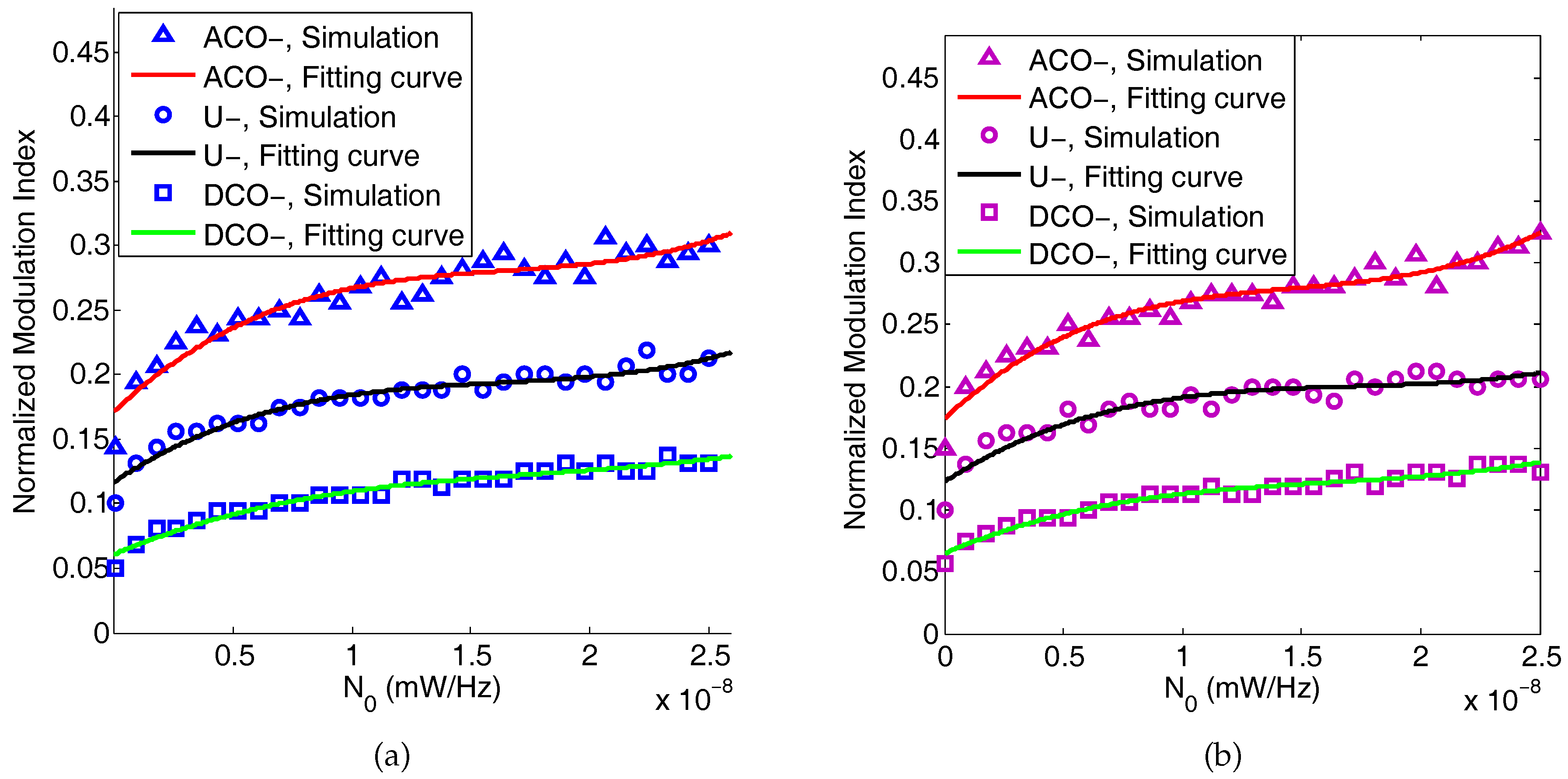
3.4. Modulation Index Optimization
4. Band-Limited Channel
5. Numerical Results
6. Conclusions
7. Future Work
Author Contributions
Funding
Conflicts of Interest
Appendix A
References
- Zeng, Z.; Fu, S.; Zhang, H.; Dong, Y.; Cheng, J. A Survey of Underwater Optical Wireless Communications. IEEE Commun. Surv. Tutor. 2017, 19, 204–238. [Google Scholar] [CrossRef]
- Kaushal, H.; Kaddoum, G. Underwater Optical Wireless Communication. IEEE Access 2016, 4, 1518–1547. [Google Scholar] [CrossRef]
- Cochenour, B.M.; Mullen, L.J.; Laux, A.E. Characterization of the Beam-Spread Function for Underwater Wireless Optical Communications Links. IEEE J. Ocean. Eng. 2008, 33, 513–521. [Google Scholar] [CrossRef]
- Zhang, H.; Dong, Y. General Stochastic Channel Model and Performance Evaluation for Underwater Wireless Optical Links. IEEE Trans. Wirel. Commun. 2016, 15, 1162–1173. [Google Scholar] [CrossRef]
- Shen, C.; Guo, Y.; Sun, X.; Liu, G.; Ho, K.; Ng, T.K.; Alouini, M.; Ooi, B.S. Going beyond 10-meter, Gbit/s underwater optical wireless communication links based on visible lasers. In Proceedings of the 2017 Opto-Electronics and Communications Conference (OECC) and Photonics Global Conference (PGC), Singapore, 31 July–4 August 2017; pp. 1–3. [Google Scholar]
- Wang, C.; Yu, H.Y.; Zhu, Y.J. A Long Distance Underwater Visible Light Communication System With Single Photon Avalanche Diode. IEEE Photonics J. 2016, 8, 7906311. [Google Scholar] [CrossRef]
- Alkhasraji, J.; Tsimenidis, C. Coded OFDM over short range underwater optical wireless channels using LED. In Proceedings of the OCEANS 2017, Aberdeen, UK, 19–22 June 2017; pp. 1–7. [Google Scholar]
- Tsonev, D.; Chun, H.; Rajbhandari, S.; McKendry, J.; Videv, S.; Gu, E.; Haji, M.; Watson, S.; Kelly, A.; Faulkner, G.; et al. A 3 Gb/s Single LED OFDM-Based Wireless VLC Link Using a Gallium Nitride μLED. IEEE Photonics Technol. Lett. 2014, 26, 637–640. [Google Scholar] [CrossRef]
- Akhoundi, F.; Salehi, J.A.; Tashakori, A. Cellular Underwater Wireless Optical CDMA Network: Performance Analysis and Implementation Concepts. IEEE Trans. Commun. 2015, 63, 882–891. [Google Scholar] [CrossRef]
- Tang, S.; Dong, Y.; Zhang, X. Impulse Response Modeling for Underwater Wireless Optical Communication Links. IEEE Trans. Commun. 2014, 62, 226–234. [Google Scholar] [CrossRef]
- Hessien, S.; Tokgoz, S.C.; Anous, N.; Boyacu, A.; Abdallah, M.; Qaraqe, K.A. Experimental Evaluation of OFDM-Based Underwater Visible Light Communication System. IEEE Photonics J. 2018, 10, 7907713. [Google Scholar] [CrossRef]
- Cicalo, S.; Tralli, V. Adaptive Resource Allocation With Proportional Rate Constraints for Uplink SC-FDMA Systems. IEEE Commun. Lett. 2014, 18, 1419–1422. [Google Scholar] [CrossRef]
- Tsiropoulou, E.E.; Kapoukakis, A.; Papavassiliou, S. Energy-efficient subcarrier allocation in SC-FDMA wireless networks based on multilateral model of bargaining. In Proceedings of the 2013 IFIP Networking Conference, Brooklyn, NY, USA, 22–24 May 2013; pp. 1–9. [Google Scholar]
- Ahani, G.; Yuan, D.; Ding, W. On SC-FDMA resource allocation with power control. In Proceedings of the 2016 IEEE 21st International Workshop on Computer Aided Modelling and Design of Communication Links and Networks (CAMAD), Toronto, ON, Canada, 23–25 October 2016; pp. 112–116. [Google Scholar] [CrossRef]
- Eleni Tsiropoulou, E.; Aggelos Kapoukakis, S.P. Uplink resource allocation in SC-FDMA wireless networks: A survey and taxonomy, Computer Networks. Comput. Netw. 2016, 96, 1–28. [Google Scholar] [CrossRef]
- Azhar, A.; Tran, T.; O’Brien, D. A Gigabit/s Indoor Wireless Transmission Using MIMO-OFDM Visible-Light Communications. IEEE Photonics Technol. Lett. 2013, 25, 171–174. [Google Scholar] [CrossRef]
- Wu, L.; Zhang, Z.; Dang, J.; Liu, H. Adaptive Modulation Schemes for Visible Light Communications. J. Lightwave Technol. 2015, 33, 117–125. [Google Scholar] [CrossRef]
- Elgala, H.; Mesleh, R.; Haas, H. Indoor optical wireless communication: Potential and state-of-the-art. IEEE Commun. Mag. 2011, 49, 56–62. [Google Scholar] [CrossRef]
- Dissanayake, S.D.; Armstrong, J. Comparison of ACO-OFDM, DCO-OFDM and ADO-OFDM in IM/DD Systems. J. Lightwave Technol. 2013, 31, 1063–1072. [Google Scholar] [CrossRef]
- Armstrong, J.; Schmidt, B.J.C. Comparison of Asymmetrically Clipped Optical OFDM and DC-Biased Optical OFDM in AWGN. IEEE Commun. Lett. 2008, 12, 343–345. [Google Scholar] [CrossRef]
- Tsonev, D.; Sinanovic, S.; Haas, H. Novel Unipolar Orthogonal Frequency Division Multiplexing (U-OFDM) for Optical Wireless. In Proceedings of the 2012 IEEE 75th Vehicular Technology Conference (VTC Spring), Yokohama, Japan, 6–9 May 2012; pp. 1–5. [Google Scholar]
- Armstrong, J.; Lowery, A.J. Power efficient optical OFDM. Electr. Lett. 2006, 42, 370–372. [Google Scholar] [CrossRef]
- Bai, J.; Li, Y.; Cheng, W.; Yang, Y.; Duan, Z.; Wang, Y. PAPR reduction for IM/DD-OFDM signals in underwater wireless optical communication system. In Proceedings of the 2018 13th IEEE Conference on Industrial Electronics and Applications (ICIEA), Wuhan, China, 31 May–2 June 2018; pp. 1837–1840. [Google Scholar]
- Lu, H.; Li, C.; Lin, H.; Tsai, W.; Chu, C.; Chen, B.; Wu, C. An 8 m/9.6 Gbps Underwater Wireless Optical Communication System. IEEE Photonics J. 2016, 8, 7906107. [Google Scholar] [CrossRef]
- Schmidl, T.M.; Cox, D.C. Robust frequency and timing synchronization for OFDM. IEEE Trans. Commun. 1997, 45, 1613–1621. [Google Scholar] [CrossRef]
- Armstrong, J. OFDM for Optical Communications. J. Lightwave Technol. 2009, 27, 189–204. [Google Scholar] [CrossRef]
- Gabriel, C.; Khalighi, M.; Bourennane, S.; Leon, P.; Rigaud, V. Channel modeling for underwater optical communication. In Proceedings of the 2011 IEEE GLOBECOM Workshops (GC Wkshps), Houston, TX, USA, 5–9 December 2011; pp. 833–837. [Google Scholar]
- Al-Kinani, A.; Wang, C.; Zhou, L.; Zhang, W. Optical Wireless Communication Channel Measurements and Models. IEEE Commun. Surv. Tutor. 2018, 20, 1939–1962. [Google Scholar] [CrossRef]
- Jamali, M.V.; Akhoundi, F.; Salehi, J.A. Performance Characterization of Relay-Assisted Wireless Optical CDMA Networks in Turbulent Underwater Channel. IEEE Trans. Wirel. Commun. 2016, 15, 4104–4116. [Google Scholar] [CrossRef]
- Akhoundi, F.; Jamali, M.V.; Hassan, N.B.; Beyranvand, H.; Minoofar, A.; Salehi, J.A. Cellular Underwater Wireless Optical CDMA Network: Potentials and Challenges. IEEE Access 2016, 4, 4254–4268. [Google Scholar] [CrossRef]
- Zhang, M.; Zhang, Z. An Optimum DC-Biasing for DCO-OFDM System. IEEE Commun. Lett. 2014, 18, 1351–1354. [Google Scholar] [CrossRef]
- Carruthers, J.B.; Kahn, J.M. Multiple-subcarrier modulation for nondirected wireless infrared communication. IEEE J. Sel. Areas Commun. 1996, 14, 538–546. [Google Scholar] [CrossRef]
- Dimitrov, S.; Sinanovic, S.; Haas, H. A comparison of OFDM-based modulation schemes for OWC with clipping distortion. In Proceedings of the 2011 IEEE GLOBECOM Workshops (GC Wkshps), Houston, TX, USA, 5–9 December 2011; pp. 787–791. [Google Scholar] [CrossRef]
- Price, R. A useful theorem for nonlinear devices having Gaussian inputs. IRE Trans. Inf. Theory 1958, 4, 69–72. [Google Scholar] [CrossRef]
- Dimitrov, S.; Sinanovic, S.; Haas, H. Double-Sided Signal Clipping in ACO-OFDM Wireless Communication Systems. In Proceedings of the 2011 IEEE International Conference on Communications (ICC), Kyoto, Japan, 5–9 June 2011; pp. 1–5. [Google Scholar]
- Zeng, L.; Minh, H.L.; O’Brien, D.; Faulkner, G.; Lee, K.; Jung, D.; Oh, Y. Equalisation for high-speed Visible Light Communications using white-LEDs. In Proceedings of the 2008 6th International Symposium on Communication Systems, Networks and Digital Signal Processing, Graz, Austria, 25 July 2008; pp. 170–173. [Google Scholar]
- Hu, S.; Gao, Q.; Gong, C.; Xu, Z. Efficient Visible Light Sensing in Eigenspace. IEEE Commun. Lett. 2018, 22, 994–997. [Google Scholar] [CrossRef]
- Fahs, B.; Chowdhury, A.J.; Hella, M.M. A 12-m 2.5-Gb/s Lighting Compatible Integrated Receiver for OOK Visible Light Communication Links. J. Lightwave Technol. 2016, 34, 3768–3775. [Google Scholar] [CrossRef]
- Popoola, W.O. Impact of VLC on Light Emission Quality of White LEDs. J. Lightwave Technol. 2016, 34, 2526–2532. [Google Scholar] [CrossRef]
- Zhang, L.; Zhang, W.; Sun, J. VLC system implementation with white LEDs. In Proceedings of the 2017 IEEE/CIC International Conference on Communications in China (ICCC), Qingdao, China, 22–24 October 2017; pp. 1–6. [Google Scholar]
- Zhang, Y.J.; Letaief, K.B. Multiuser adaptive subcarrier-and-bit allocation with adaptive cell selection for OFDM systems. IEEE Trans. Wirel. Commun. 2004, 3, 1566–1575. [Google Scholar] [CrossRef]


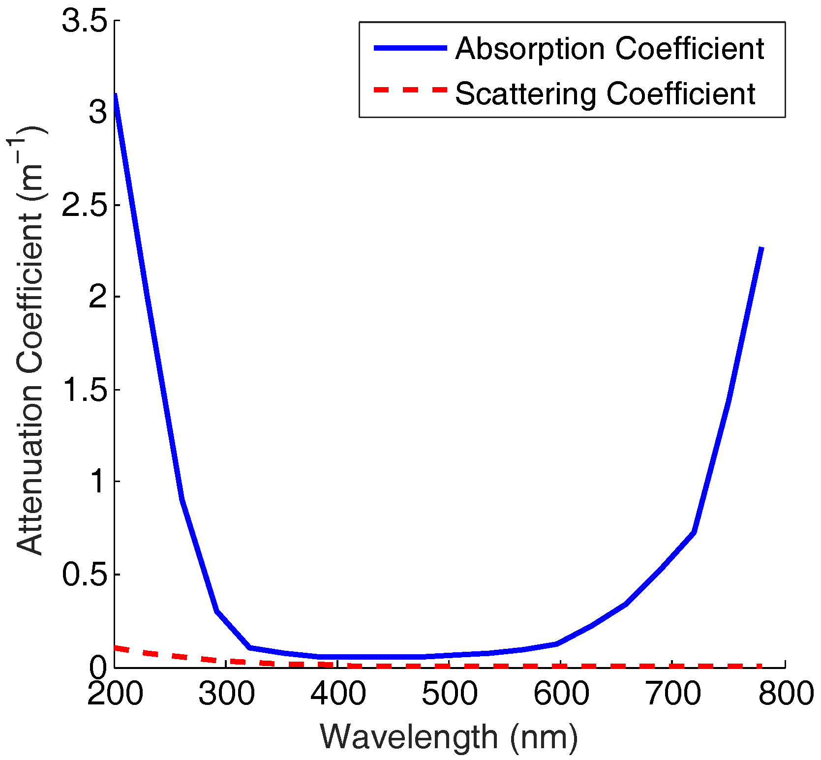
| : | absorption attenuation |
| : | scattering attenuation |
| : | clipping coefficient |
| : | modulation index |
| h: | channel loss |
| : | size of the photodetector |
| d: | propagation distance |
| N: | Number of subcarriers for OFDM |
| sample for the DCO-OFDM signal | |
| sample for the UCO-OFDM signal | |
| sample for the ACO-OFDM signal | |
| DC bias for DCO-OFDM | |
| probability density function of the DCO-OFDM signal | |
| probability density function of the UCO-OFDM signal | |
| probability density function of the ACO-OFDM signal | |
| average optical power | |
| peak transmitted power |
| Water Types | Absorption (m) | Scattering (m) |
|---|---|---|
| Pure Sea Water | 0.053 | 0.003 |
| Clear Ocean | 0.114 | 0.037 |
| Coastal Ocean | 0.179 | 0.219 |
| Turbid Harbor | 0.295 | 1.875 |
| Responsivity | 0.45 A/W |
| Equivalent area of the PD using a lens | |
| Thermal noise density, | mW/Hz |
| Radiation optical power of each lamp, | 10 W |
| LED semi-angle | 30° |
| 0.053 () | |
| 0.003 () | |
| 0.056 () | |
| Number of subcarriers, N | 128 |
© 2019 by the authors. Licensee MDPI, Basel, Switzerland. This article is an open access article distributed under the terms and conditions of the Creative Commons Attribution (CC BY) license (http://creativecommons.org/licenses/by/4.0/).
Share and Cite
Lian, J.; Gao, Y.; Wu, P.; Lian, D. Orthogonal Frequency Division Multiplexing Techniques Comparison for Underwater Optical Wireless Communication Systems. Sensors 2019, 19, 160. https://doi.org/10.3390/s19010160
Lian J, Gao Y, Wu P, Lian D. Orthogonal Frequency Division Multiplexing Techniques Comparison for Underwater Optical Wireless Communication Systems. Sensors. 2019; 19(1):160. https://doi.org/10.3390/s19010160
Chicago/Turabian StyleLian, Jie, Yan Gao, Peng Wu, and Dianbin Lian. 2019. "Orthogonal Frequency Division Multiplexing Techniques Comparison for Underwater Optical Wireless Communication Systems" Sensors 19, no. 1: 160. https://doi.org/10.3390/s19010160
APA StyleLian, J., Gao, Y., Wu, P., & Lian, D. (2019). Orthogonal Frequency Division Multiplexing Techniques Comparison for Underwater Optical Wireless Communication Systems. Sensors, 19(1), 160. https://doi.org/10.3390/s19010160