Radar Emitter Recognition Based on the Energy Cumulant of Short Time Fourier Transform and Reinforced Deep Belief Network


Abstract
1. Introduction
2. Problem Description and Hypothesis
- The intra-pulse signals stem from sorted signals, and the influence of false alarms and the missed detections are not considered.
- The five common parameters of radar emitter are known a priori. The intra-pulse signal is simplex, and the parameters of the signal remain invariable during the PW.
- This work aims to solve the problem based on the sample database by offline training, so the recognition of radar emitter without database information and the online learning are not considered.
3. Radar Emitter Intra-Pulse Signals
3.1. Frequency Modulated Signal
3.1.1. Discrete Frequency Modulated Signal
3.1.2. Continuous Frequency Modulated Signal
3.2. Phase Modulated Signal
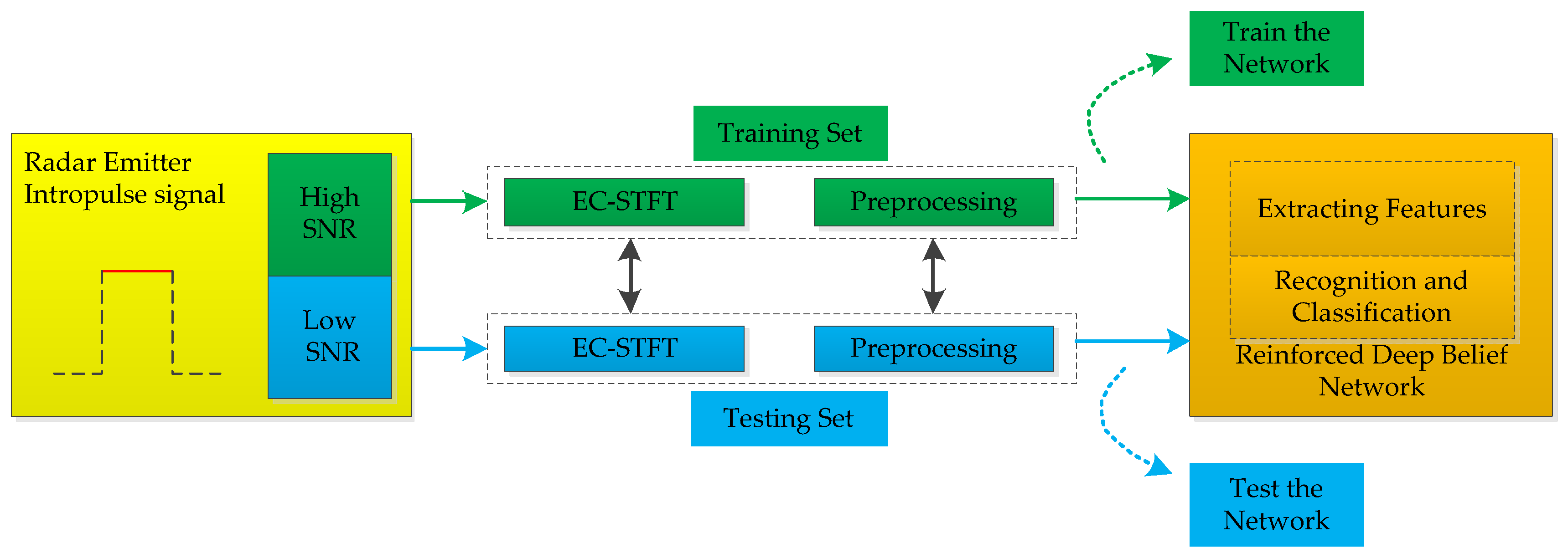
4. The Proposed Recognition Method Analysis
4.1. Feature Selection and Calculation
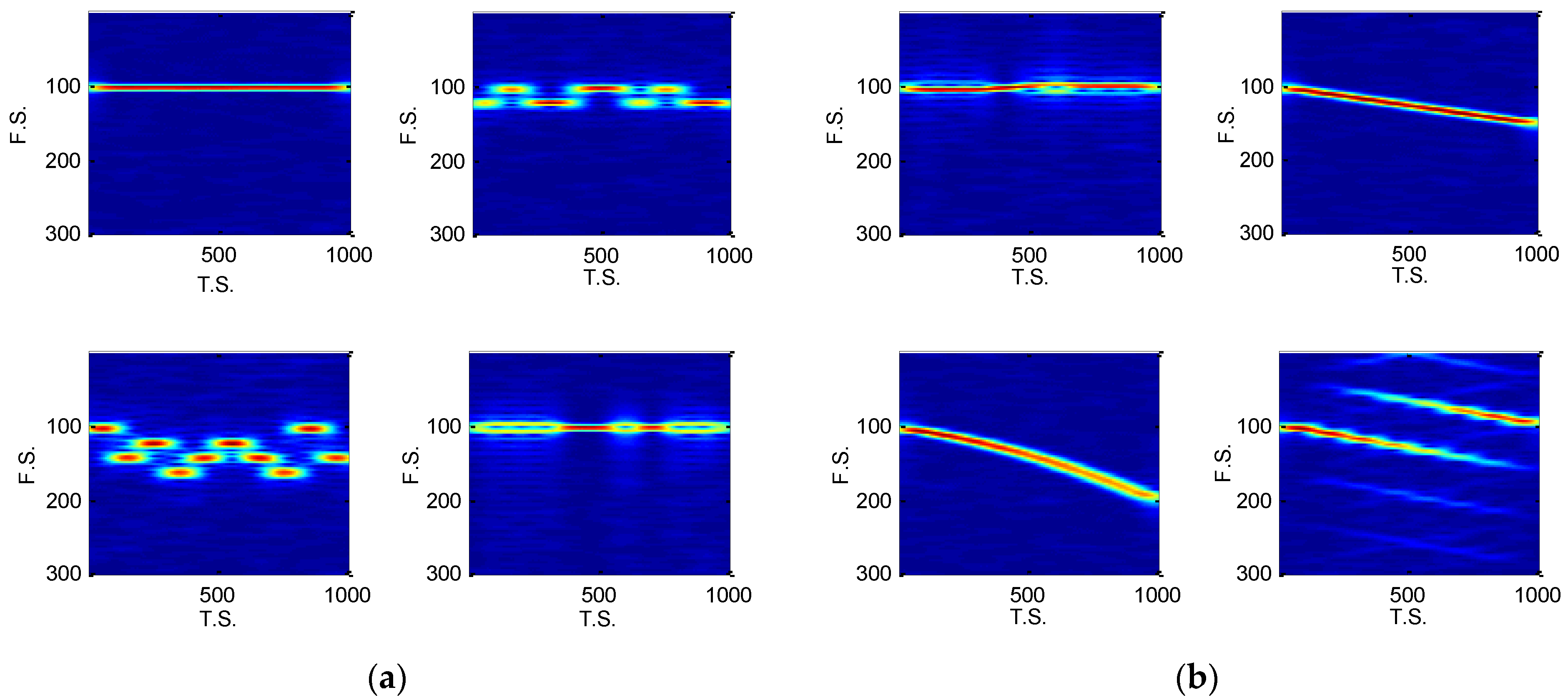
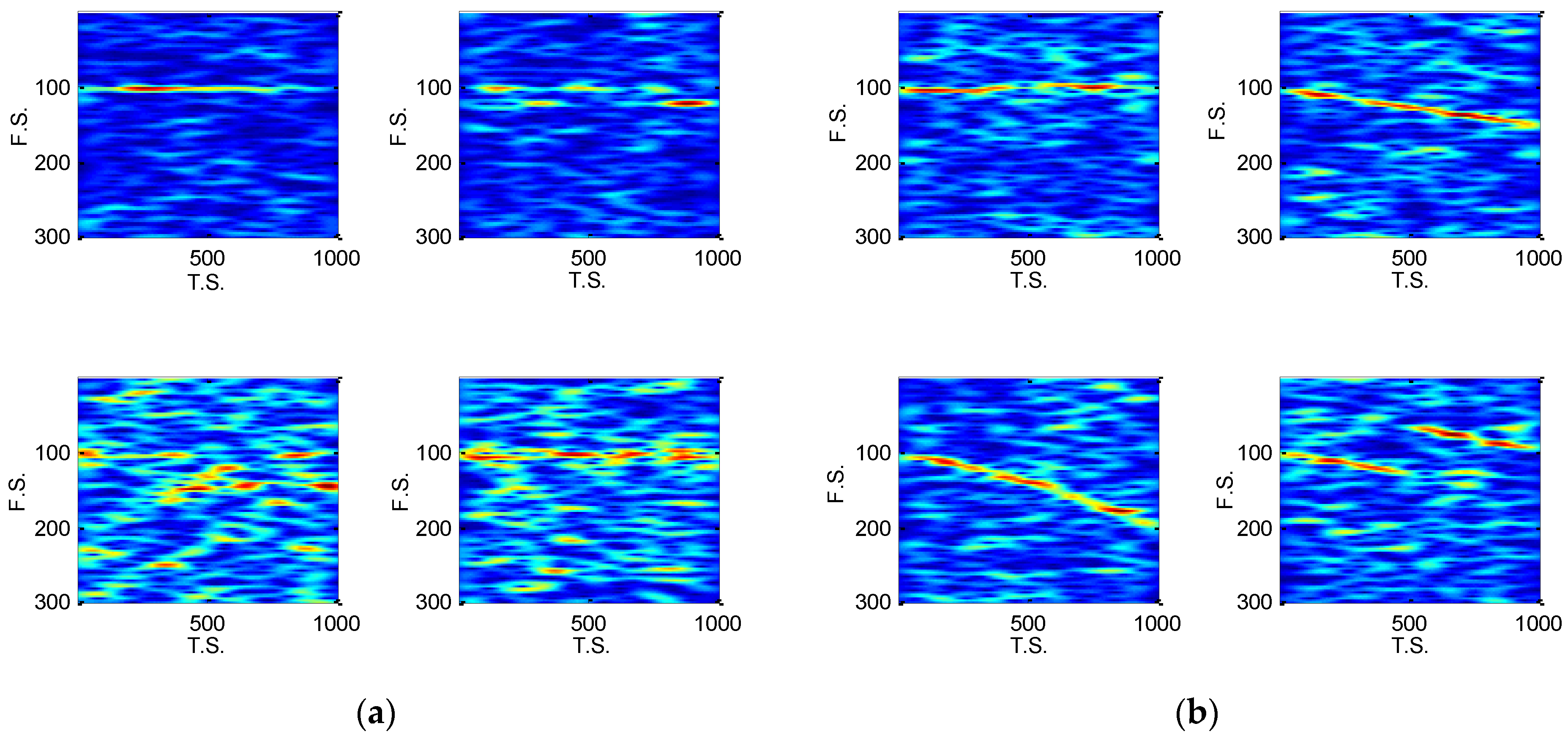
4.1.1. Short Time Fourier Transform
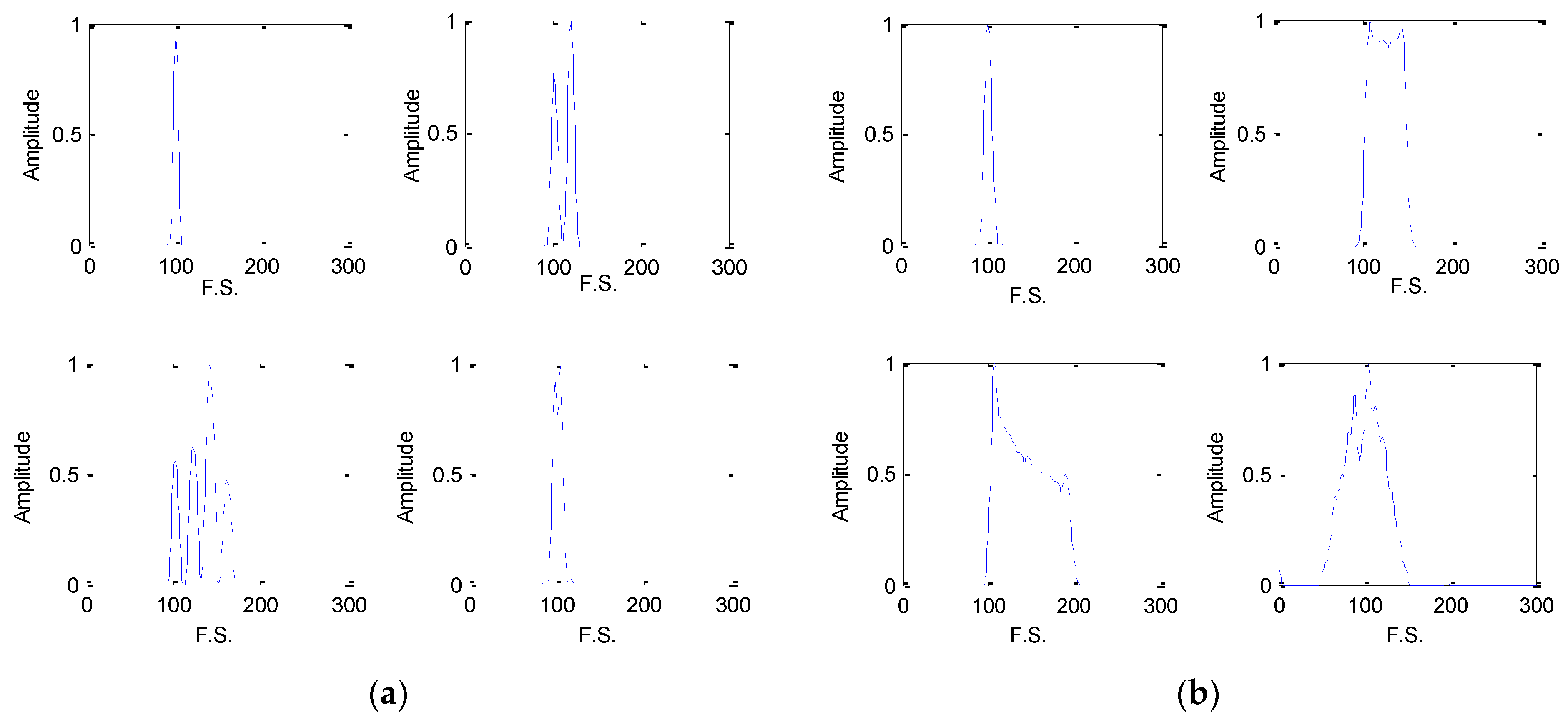
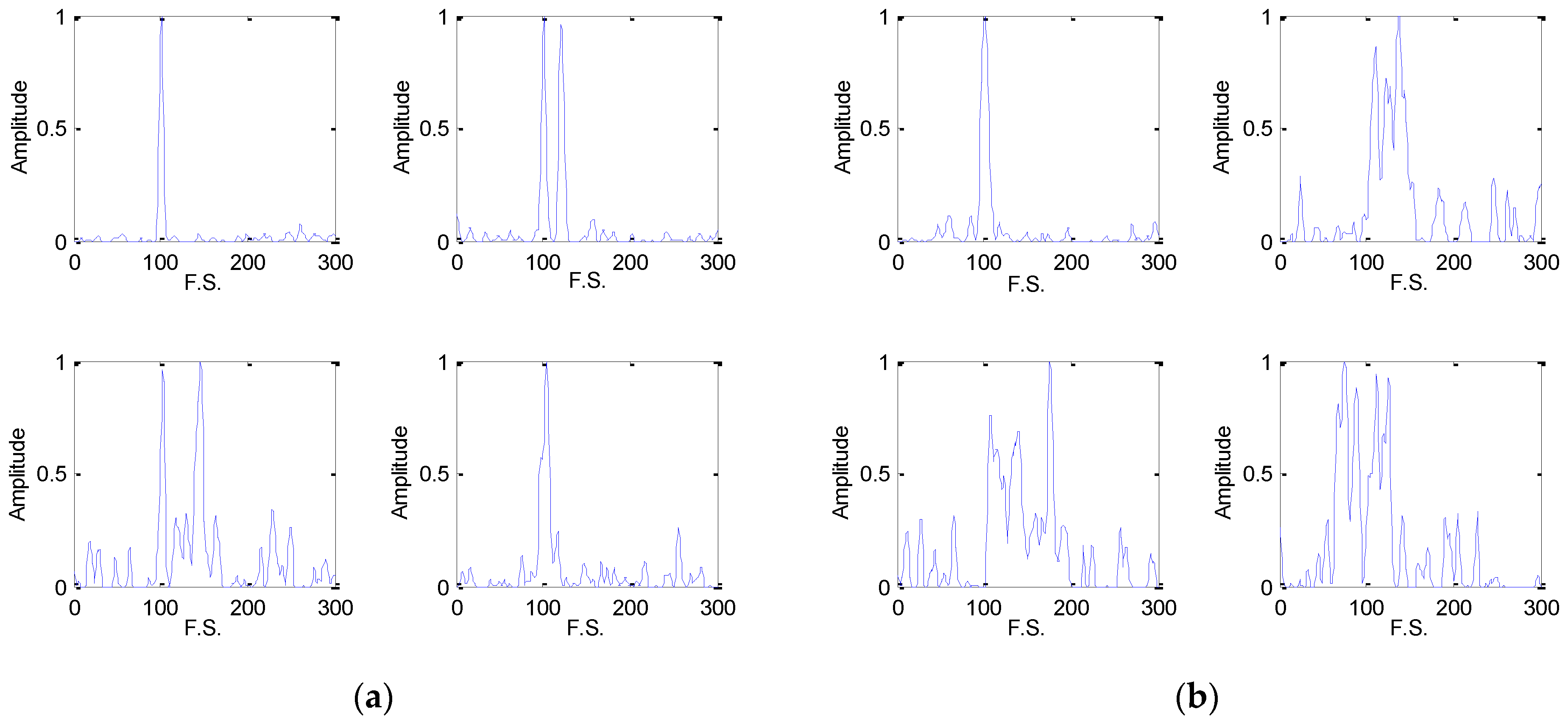
4.1.2. Energy Cumulant of Short Time Fourier Transform
4.2. Feature Preprocessing
- The carrier frequency of the intra-pulse signal is the intermediate frequency. When it is at other frequency points, it will be moved to .
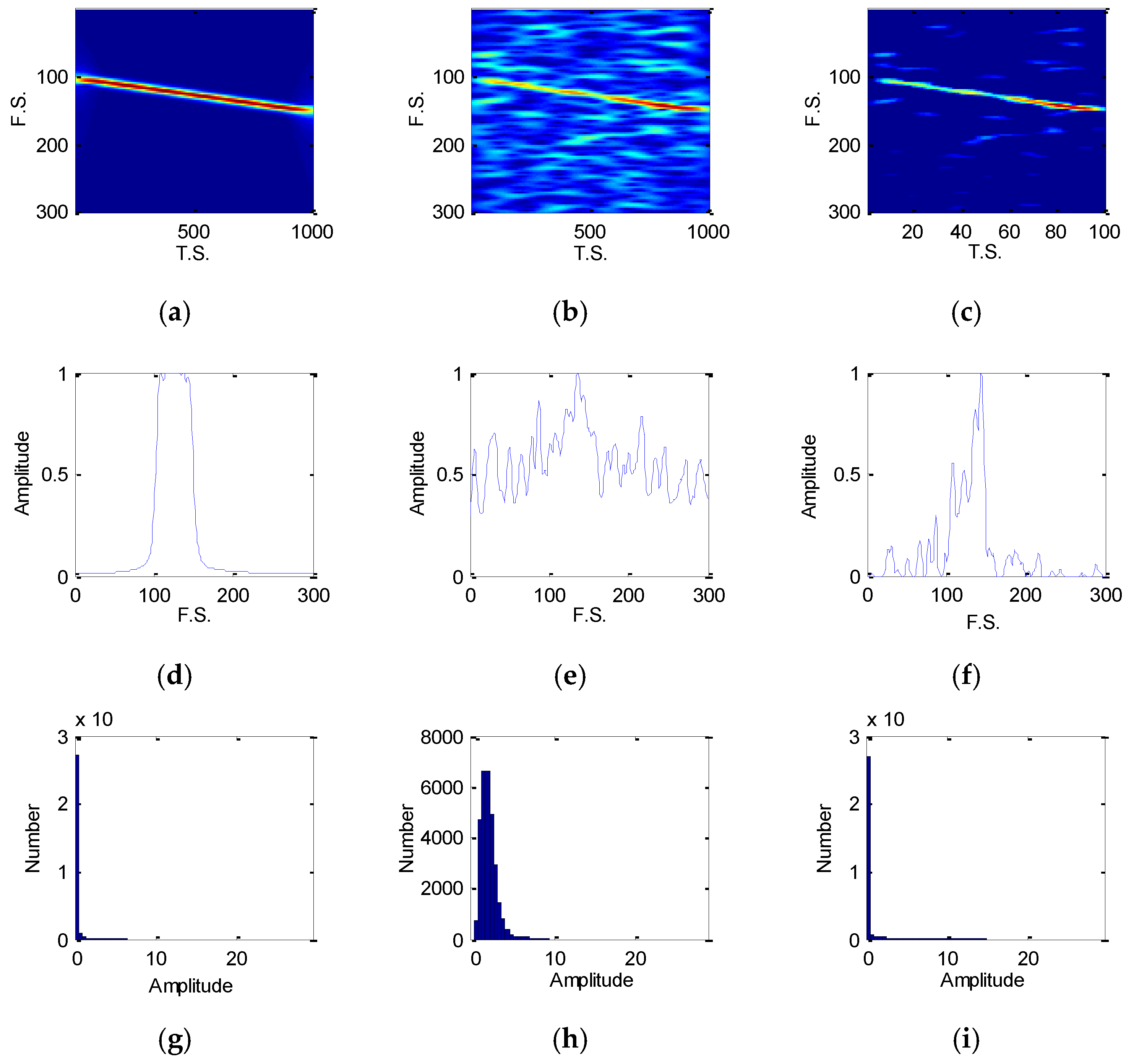
- Suppose is the TFD matrix of a noisy radar emitter intra-pulse signal via STFT in a large size. And a cutting and sampling on are conducted with the result of . To process the noise, is transformed into a vector, , in which is the raw vector of . For , a zero-mean scaling is completed by:where the is mean of all the elements of , and gets the variance of all elements of . Then the denoising is operated by:where and removes the weak noisy points. Apparently, the Equation (10) just removes a part of noise. In order to get better denoising performance, the Equations (9) and (10) are repeated six times [3].
4.3. Reinforced Deep Belief Networks
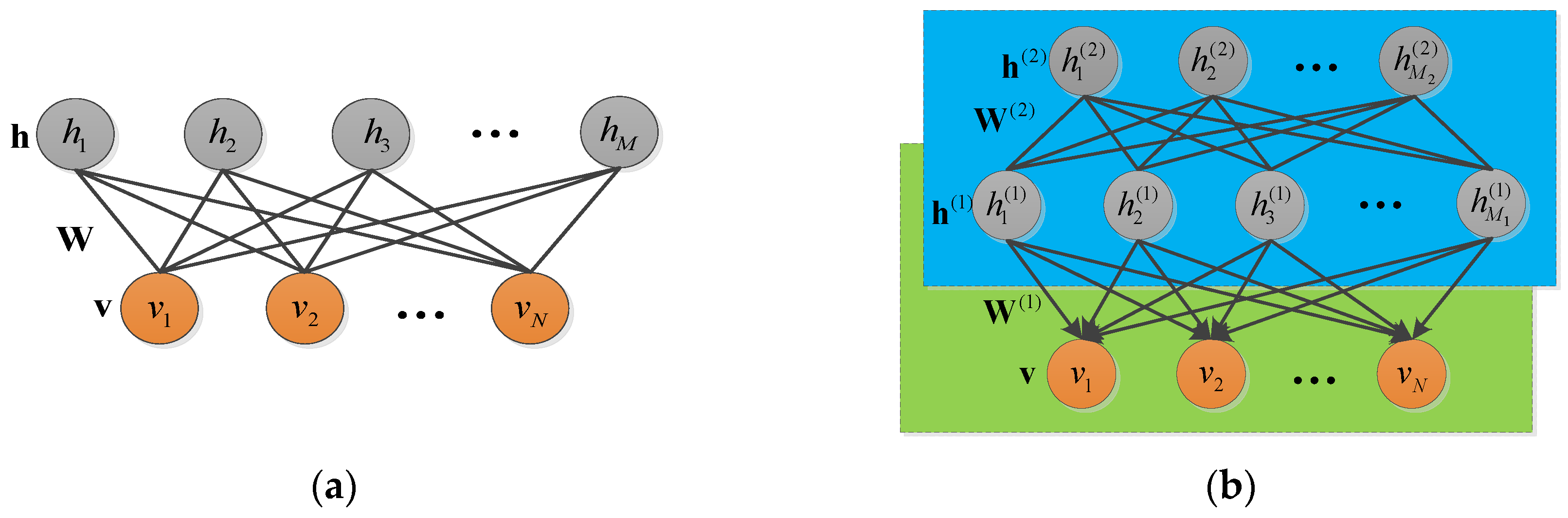
4.3.1. Restricted Boltzmann Machine and Deep Belief Network
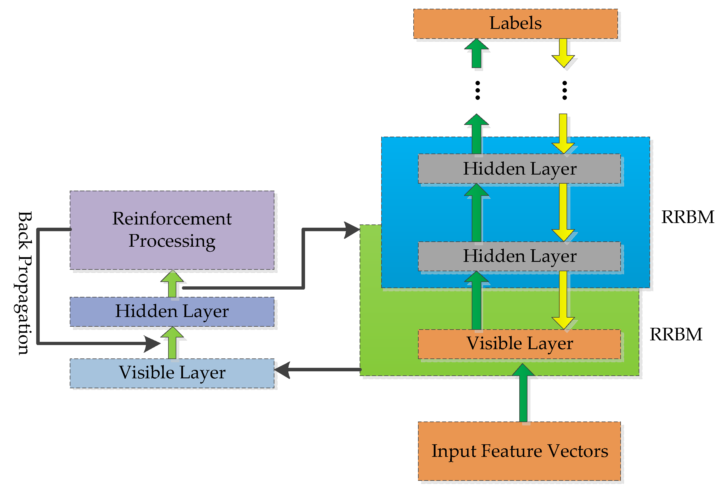
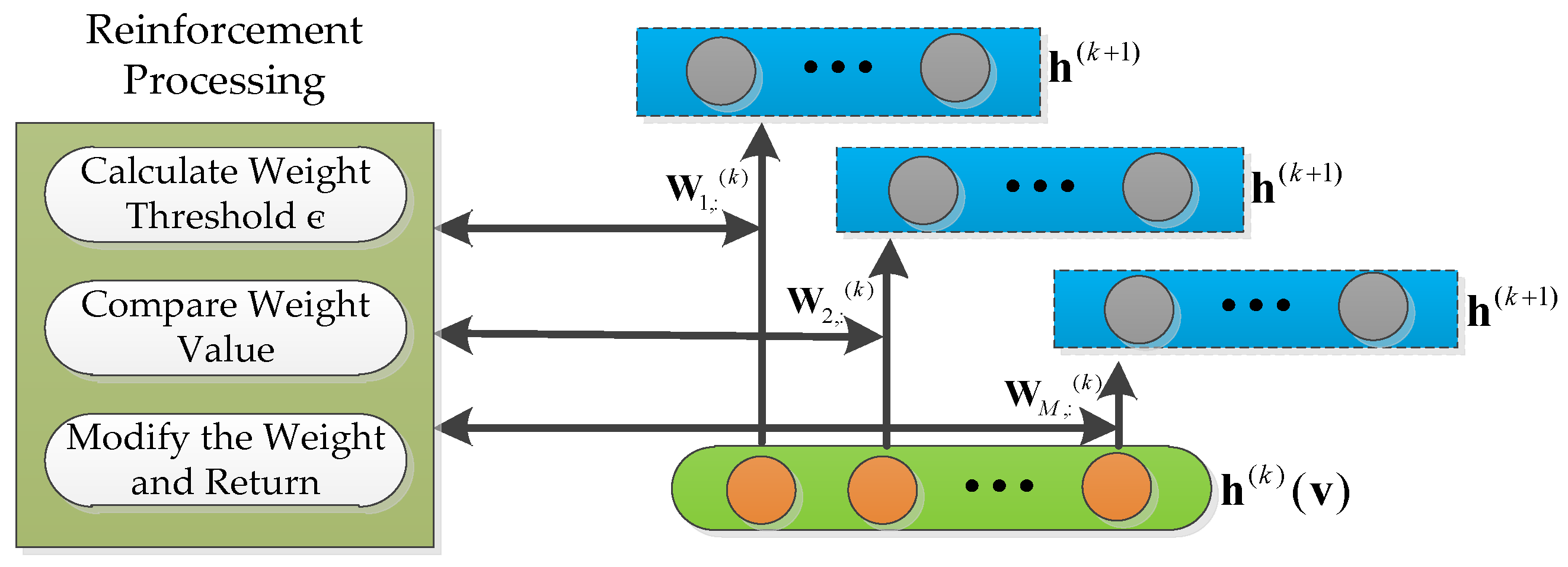
4.3.2. Reinforced Deep Belief Network
| Algorithm 1. The reinforcement algorithm on in RRBN. |
| Input: Weight matrix ; |
| Learning rate ; |
| Tuning factor . |
| Process: |
| 1. , , ; |
| 2. |
| 3. for do |
| 4. for do |
| 5. if do |
| 6. ; |
| 7. else |
| 8. ; |
| 9. end if |
| 10. end for |
| 11. end for |
| Output: Reinforced weight matrix . |
5. Simulations and Discussions
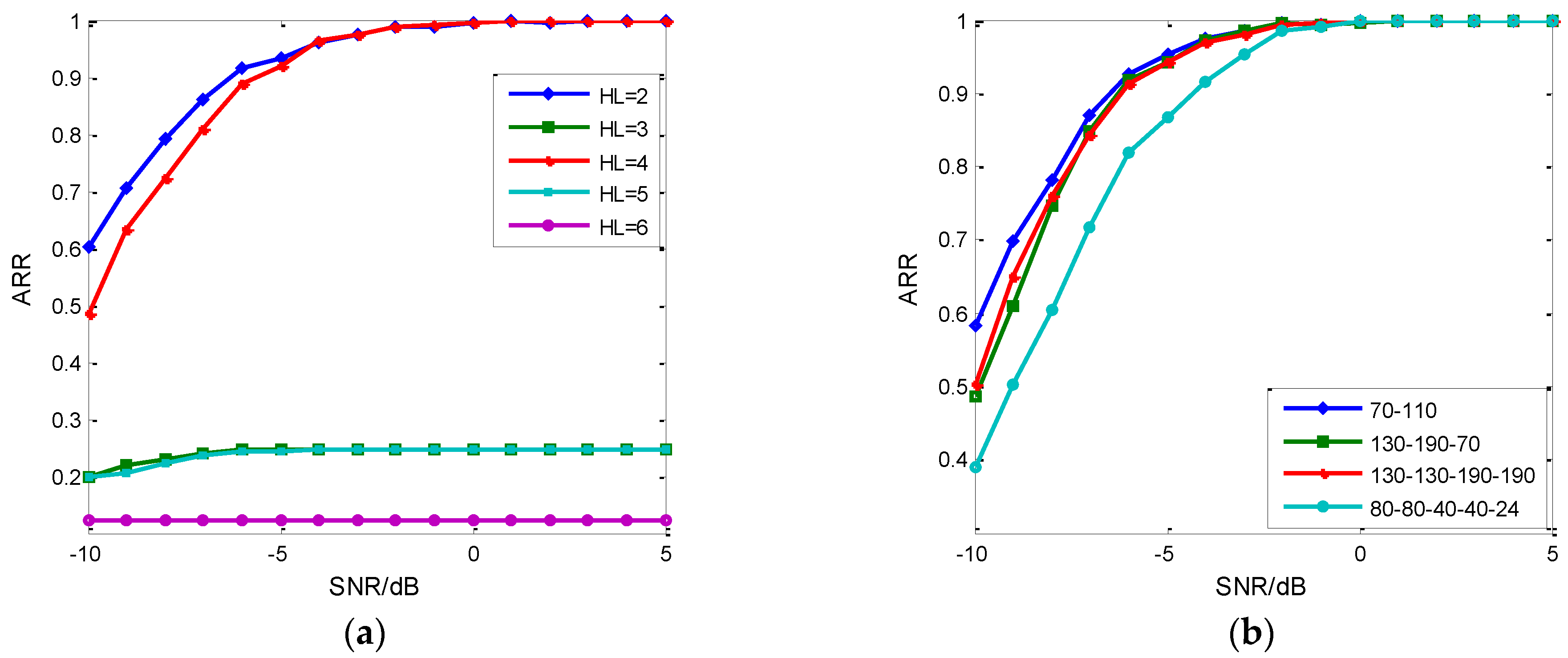
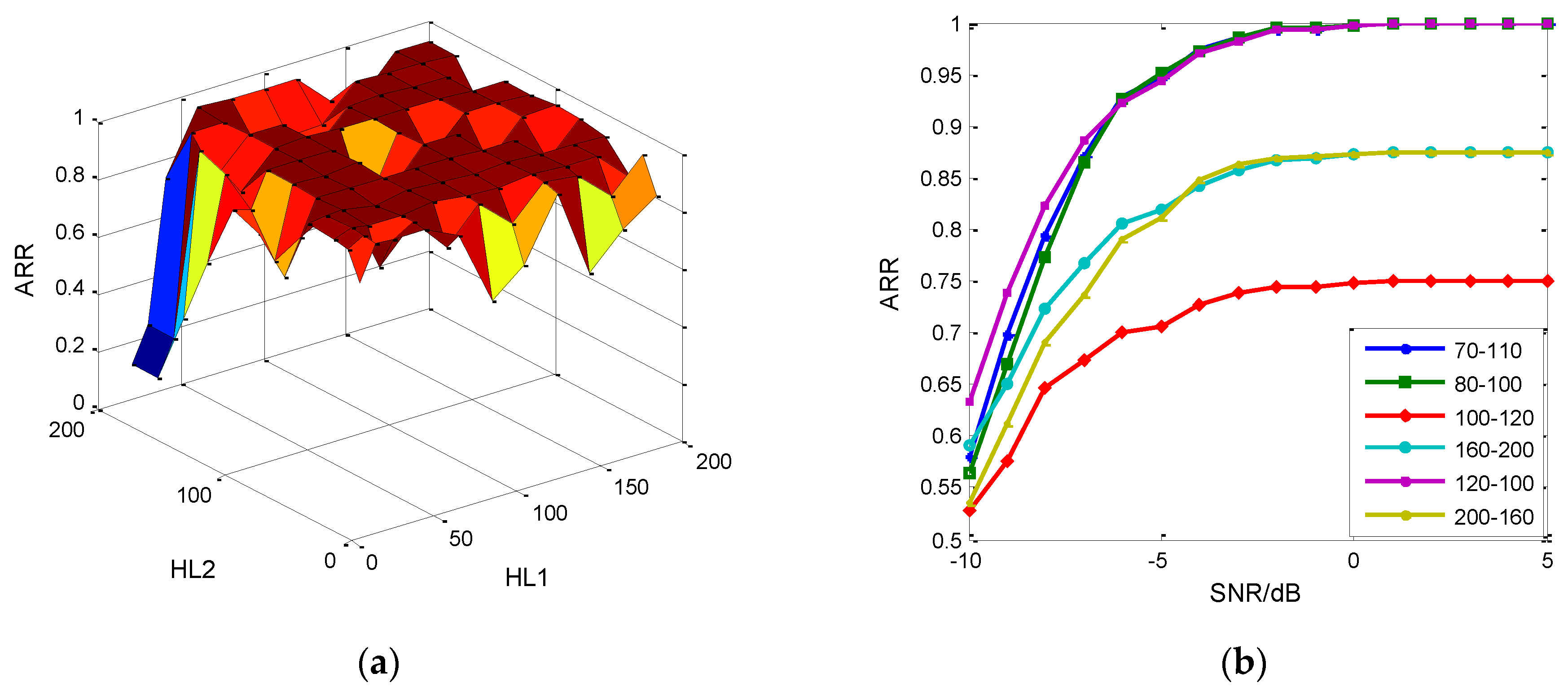
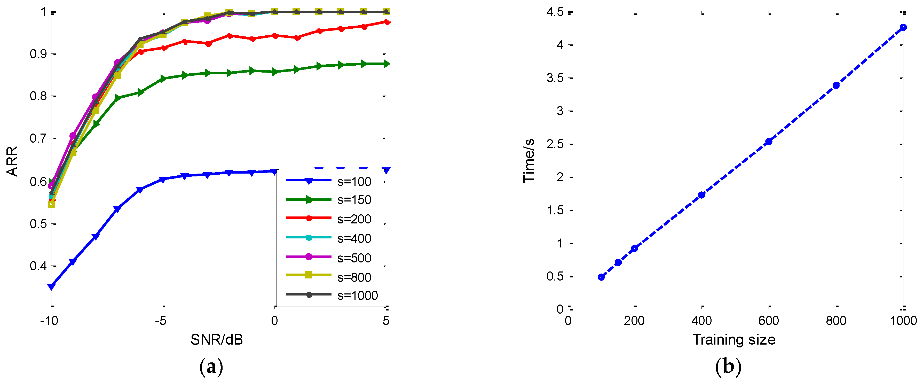
5.1. The Network Validation
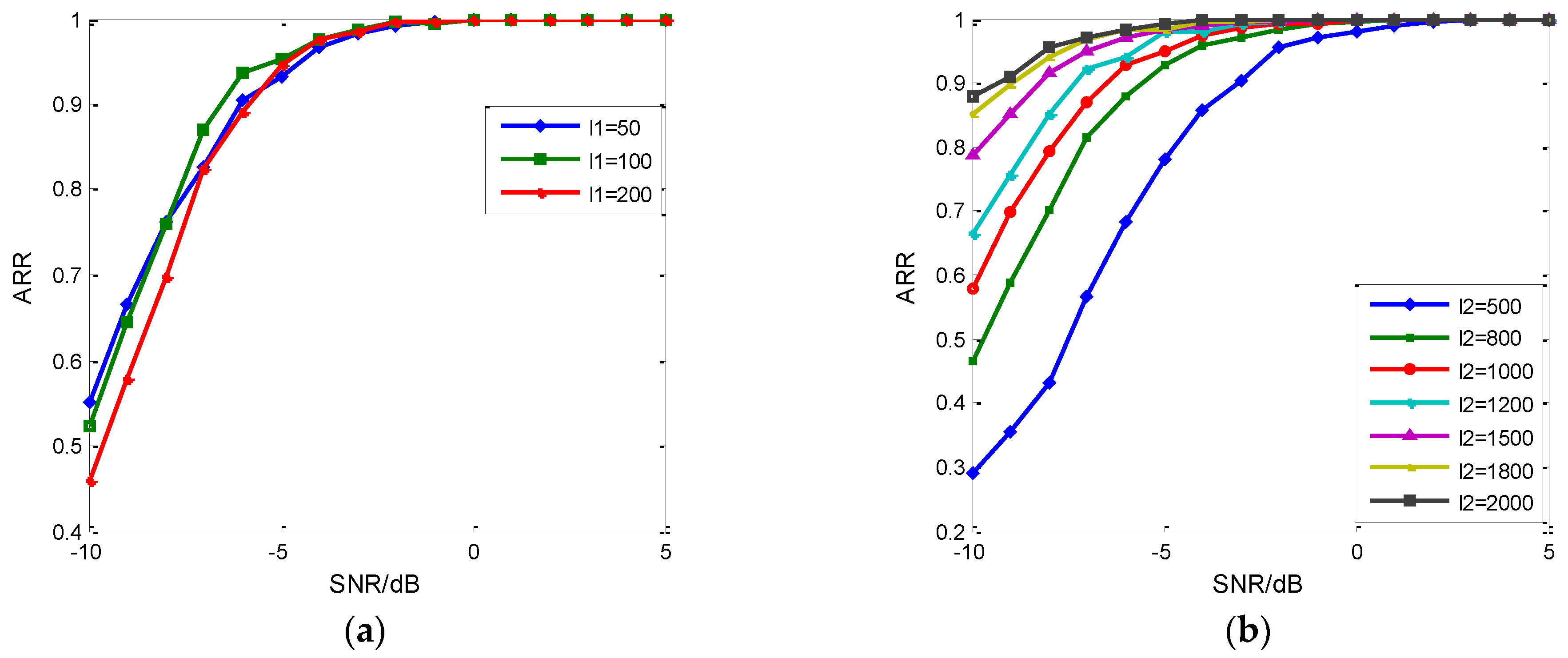
5.2. The Fearture Set Discussion
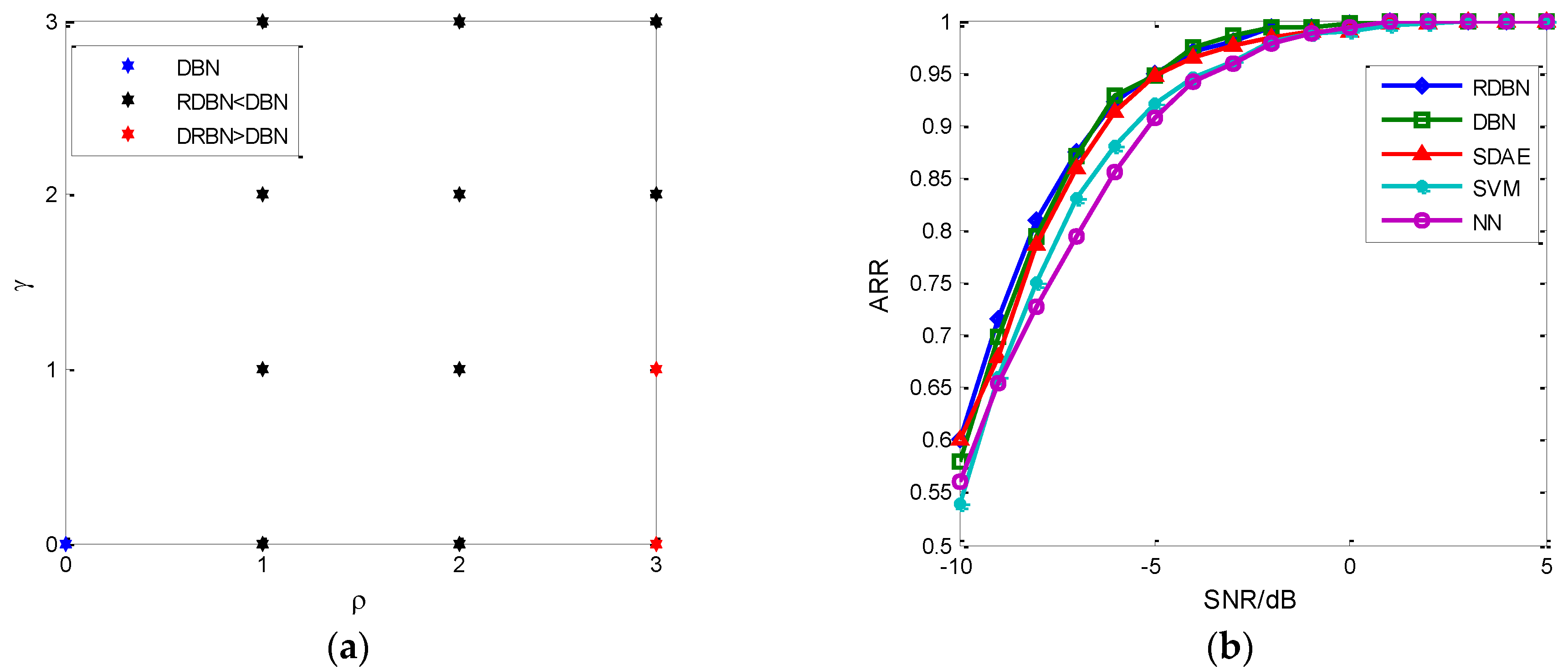
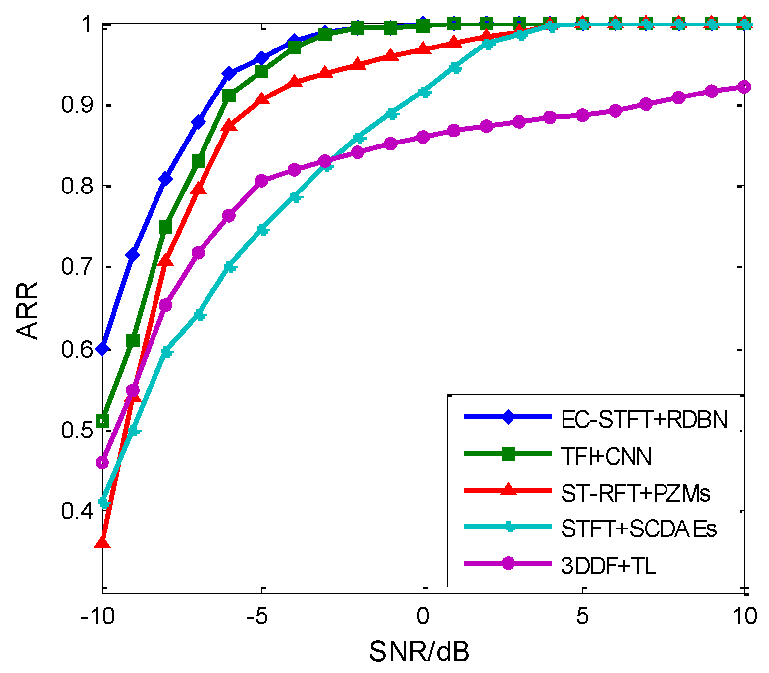
5.3. The Method Performance Comparison
6. Conclusions
Author Contributions
Funding
Conflicts of Interest
Nomenclature
| AOA | Angle of arrival |
| ARR | Average recognition rate |
| AWGN | Addictive white Gaussian noise |
| CD | Contrastive divergence |
| CFM | Continuous frequency modulation |
| CNN | Convolutional neural network |
| CWD | Choi-Williams distribution |
| DFM | Discrete frequency modulation |
| EC-STFT | Energy cumulant of short time Fourier transform |
| FT | Fourier transform |
| IF | Intermediate frequency |
| NN | Neural network |
| PA | Pulse amplitude |
| RBM | Restricted Boltzmann machine |
| RDBN | Reinforced deep belief network |
| RF | Radio frequency |
| RRBM | Reinforced restricted Boltzmann machine |
| SDAE | Stacked denoising autoencoder |
| SEI | Specific emitter identification |
| SRR | Single recognition rate |
| STFT | Short time Fourier transform |
| SVM | Support vector machine |
| TFD | Time-frequency distribution |
| TOA | Time of arrival |
| WVD | Wigner-Ville distribution |
Appendix A
| Algorithm A1. Matlab Code of Computation on EC-STFT. |
| function [ecq,n] = ecstft(x) |
| % ECSTFT: Energy cumulation of short time Fourier transform |
| % x: signal. |
| % n: frequency sequence. |
| % ecq: the sequence of energy cumulation of short time Fourier transform |
| [tfr,t,f] = tfrstft(x); % The computation of STFT on x is based on the method proposed by Auger F., 1995 |
| tfr_abs = abs(tfr); |
| q = length(t); |
| m = 1:q; |
| p = length(f)/2; |
| n = 1:p; |
| ecq = zeros(1,p); |
| for i = 1:p |
| ecq(i) = sum(tfr_abs(i,:)); |
| end; |
| end; |
References
- Whittall, N.J. Signal sorting in ESM system. IEE Proc. Commun. Radar Signal Process. 1985, 132, 226–228. [Google Scholar] [CrossRef]
- Zhou, Z.W.; Huang, G.M.; Chen, H.Y.; Gao, J. Automatic radar emitter waveform recognition based on deep convolutional denoising auto-encoders. Circuit Syst. Signal Process. 2018, 34, 1–15. [Google Scholar]
- Wang, X.B.; Huang, G.M.; Zhou, Z.W.; Gao, J. Radar emitter recognition based on the short time Fourier transform and convolutional neural networks. In Proceedings of the 10th International Congress on Image and Signal Processing, BioMedical Engineering and Informatics (CISP-BMEI), Shanghai, China, 14–16 October 2017. [Google Scholar]
- Zhou, C.; Huang, G.M.; Shan, H.C.; Gao, J. Bias compensation based on maximum likelihood estimation for passive location using TDOA and FDOA measurements. Acta Aeronaut. Astronaut. Sin. 2015, 36, 979–986. [Google Scholar]
- Qiu, H.; Huang, G.M.; Gao, J. Variational Bayesian labeled multi-Bernoulli filter with unknown sensor noise statistics. Chin. J. Aeronaut. 2016, 29, 1378–1384. [Google Scholar]
- Guo, Q.; Nan, P.L. Method for feature extraction of radar full pulses based on EMD and chaos detection. J. Commun. Netw. 2014, 16, 92–97. [Google Scholar] [CrossRef]
- Yang, Z.T.; Wu, Z.L.; Yin, Z.D.; Quan, T.; Sun, H. Hybrid radar emitter recognition based on rough k-means classifier and relevance vector machine. Sensors 2013, 13, 848–864. [Google Scholar] [CrossRef] [PubMed]
- Han, J.; He, M.H.; Tang, Z.K.; Wang, J. Estimating in-pulse characteristics of radar signal based on multi-index. Chin. J. Electron. 2011, 20, 187–191. [Google Scholar]
- Skolnik, M.I. Radar Handbook, 3rd ed.; The McGraw-Hill Companies Inc.: New York, NY, USA, 2008; ISBN 978-0-07-148547-0. [Google Scholar]
- Lundén, J.; Koivunen, V. Automatic radar waveform recognition. IEEE J. Sel. Top. Signal Process. 2007, 1, 124–136. [Google Scholar] [CrossRef]
- Guo, Q.; Nan, P.L.; Zhang, X.Y.; Zhao, Y.; Wan, J. Recognition of radar emitter signals based on SVD and AF main ridge slice. J. Commun. Netw. 2015, 17, 491–498. [Google Scholar]
- Kishore, T.R.; Rao, K.D. Automatic intra-pulse modulation classification of advanced LPI radar Waveforms. IEEE Trans. Aerosp. Electron. Syst. 2017, 53, 901–914. [Google Scholar] [CrossRef]
- Ru, X.H.; Liu, Z.; Jiang, W.L.; Huang, Z.T. Recognition performance analysis of instantaneous phase and its transformed features for radar emitter identification. IET Radar Sonar Navig. 2016, 10, 945–952. [Google Scholar] [CrossRef]
- Wang, X.Q.; Liu, J.Y.; Meng, H.D.; Liu, Y.M. A method for radar emitter signal recognition based on time-frequnency atom features. J. Infrared Millim. Waves 2011, 30, 566–570. [Google Scholar] [CrossRef]
- Kang, N.X.; He, M.H.; Han, J.; Wang, B.Q. Radar emitter fingerprint recognition based on bispectrum and SURF feature. In Proceedings of the CIE International Conference on Radar, Guangzhou, China, 10–13 October 2016. [Google Scholar]
- Zachepitskii, A.A.; Krichigin, A.V. Maximum radar range versus the statistical characteristics of fluctuating targets and detection quality indices. J. Commun. Technol. Electron. 2017, 62, 507–511. [Google Scholar] [CrossRef]
- Li, H.B.; Jing, W.; Bai, Y. Radar emitter recognition based on deep learning architecture. In Proceedings of the CIE International Conference on Radar, Guangzhou, China, 10–13 October 2016. [Google Scholar]
- Anderson, J.A.; Gately, M.T.; Penz, P.A.; Collins, D.R. Radar signal categorization using a neural network. Proc. IEEE 1990, 78, 1646–1657. [Google Scholar] [CrossRef]
- Zhu, W.G.; Li, M.; Zeng, C.Z. Research on online learning of radar emitter recognition based on Hull Vector. In Proceedings of the IEEE Second International Conference on Data Science in Cyberspace (DSC), Shenzhen, China, 26–29 June 2017. [Google Scholar]
- Mendis, G.J.; Wei, J.; Madanayake, A. Deep learning cognitive radar for micro UAS detection and classification. In Proceedings of the 2017 Cognitive Communications for Aerospace Applications Workshop (CCAA), Cleveland, OH, USA, 27–28 June 2017. [Google Scholar]
- Yang, Z.T.; Qiu, W.; Sun, H.J.; Nallanathan, A. Robust radar emitter recognition based on the three-dimensional distribution feature and transfer learning. Sensors 2016, 16, 289. [Google Scholar] [CrossRef] [PubMed]
- Wang, C.; Wang, J.; Zhang, X.D. Automatic radar waveform recognition based on time-frequency analysis and convolutional neural network. In Proceedings of the IEEE International Conference on Acoustics, Speech and Signal Processing, New Orleans, LA, USA, 5–9 March 2017. [Google Scholar]
- Ma, X.R.; Liu, D.; Shan, Y.L. Intra-pulse modulation recognition using short-time ramanujan Fourier transform spectrogram. EURASIP J. Adv. Signal Process. 2017, 42, 9–19. [Google Scholar] [CrossRef]
- Zhang, M.; Diao, M.; Guo, L.M. Convolutional neural networks for automatic cognitive radio waveform recognition. IEEE Access 2017, 5, 11074–11082. [Google Scholar] [CrossRef]
- Goodfellow, I.; Bengio, Y.; Courville, A. Deep Learning; MIT Press: Cambridge, MA, USA, 2017; Chapter 20; ISBN 978-0-262-03561-3. [Google Scholar]
- Husain, F.; Dellen, B.; Torras, C. Action recognition based on efficient deep feature learning in the Spatio-Temporal domain. IEEE Robot. Autom. Lett. 2016, 1, 984–991. [Google Scholar] [CrossRef]
- Hinton, G.E.; Osindero, S.; Teh, Y.W. A fast learning algorithm for deep belief nets. Neural Comput. 2006, 18, 1527–1542. [Google Scholar] [CrossRef] [PubMed]
- Hinton, G.E.; Salakhutdinov, R. Reducing the dimensionality of data with neural networks. Science 2006, 5786, 504–507. [Google Scholar] [CrossRef] [PubMed]
- Ling, Z.H.; Deng, L.; Yu, D. Modeling spectral envelopes using restricted Boltzmann machines and deep belief networks for statistical parametric speech synthesis. IEEE Trans. Audio Speech Lang. Process. 2013, 21, 2129–2139. [Google Scholar] [CrossRef]
- Yang, H.H.; Shen, S.; Yao, X.H.; Sheng, M.; Wang, C. Competitive deep belief network for underwater acoustic target recognition. Sensors 2018, 18, 952. [Google Scholar] [CrossRef] [PubMed]
- Zhang, X.D.; Bao, Z. Non-Stationary Signal Analysis and Processing, 1st ed.; National Defence Industry Press: Beijing, China, 1998; Chapter 2; ISBN 7-118-01941-0. [Google Scholar]
- Aubel, C.; Stotz, D.; Bölcskei, H. A theory of super-resolution from short-time Fourier transform measurements. J. Fourier Anal. Appl. 2018, 1, 45–107. [Google Scholar] [CrossRef]
- Mateo, C.; Talavera, J.A. Short-time Fourier transform with the window size fixed in the frequency domain. Digit. Signal Process. 2018, 77, 13–21. [Google Scholar] [CrossRef]
- Torres, L.; Jiménez-Cabas, J.; Gómez-Aguilar, J.F.; Pérez-Alcazar, P. A simple spectral observer. Math. Comput. Appl. 2018, 2, 23–36. [Google Scholar]
- Mateo, C.; Talavera, J.A. Short-time Fourier transform with the window size fixed in the frequency domain (STFT-FD): Implementation. SoftwareX 2018, 11, 5–9. [Google Scholar] [CrossRef]
- Auger, F.; Flandrin, F. Improving the readability of time-frequency and time-scale representations by the reassignment method. IEEE Trans. Signal Process. 1995, 43, 1068–1089. [Google Scholar] [CrossRef]
- Zhang, G.Z. Research on Emitter Identification. Ph.D. Thesis, National University of Defense Technology, Changsha, China, March 2005. [Google Scholar]
- Wang, X.B.; Huang, G.M.; Zhou, Z.W.; Tian, W.; Yao, J.L.; Gao, J. Radar emitter intra-pulse signal blind sorting under modified wavelet denoising. In Proceedings of the IET International Radar Conference, Nanjing, China, 17–19 October 2018. accepted. [Google Scholar]


| Layer | 2 | 3 | 4 | 5 | 6 |
|---|---|---|---|---|---|
| Time/s (a) | 4.585 | 7.237 | 10.175 | 12.512 | 14.352 |
| Time/s (b) | 2.365 | 5.174 | 8.396 | 3.689 | - |
| SRR (%) | NS | BFSK | QFSK | BPSK | QPSK | LFM1 | LFM2 | LFM3 | NLFM | FRANK | Total |
|---|---|---|---|---|---|---|---|---|---|---|---|
| NS | 100 | 0 | 0 | 0 | 0 | 0 | 0 | 0 | 0 | 0 | 100 |
| BFSK | 0 | 100 | 0 | 0 | 0 | 0 | 0 | 0 | 0 | 0 | 100 |
| QFSK | 0 | 0 | 100 | 0 | 0 | 0 | 0 | 0 | 0 | 0 | 100 |
| BPSK | 0 | 0 | 0 | 99 | 1 | 0 | 0 | 0 | 0 | 0 | 100 |
| QPSK | 0 | 0 | 0 | 5 | 95 | 0 | 0 | 0 | 0 | 0 | 100 |
| LFM1 | 0 | 0 | 0 | 0 | 0 | 100 | 0 | 0 | 0 | 0 | 100 |
| LFM2 | 0 | 0 | 0.5 | 0 | 0 | 0 | 79.5 | 1 | 19 | 0 | 100 |
| LFM3 | 0 | 0 | 0 | 0 | 0 | 0 | 0 | 100 | 0 | 0 | 100 |
| NLFM | 0 | 0 | 1 | 0 | 0 | 0.5 | 9 | 0 | 89.5 | 0 | 100 |
| FRANK | 0 | 0 | 0 | 0 | 0 | 0 | 0 | 0 | 0 | 100 | 100 |
© 2018 by the authors. Licensee MDPI, Basel, Switzerland. This article is an open access article distributed under the terms and conditions of the Creative Commons Attribution (CC BY) license (http://creativecommons.org/licenses/by/4.0/).
Share and Cite
Wang, X.; Huang, G.; Zhou, Z.; Tian, W.; Yao, J.; Gao, J. Radar Emitter Recognition Based on the Energy Cumulant of Short Time Fourier Transform and Reinforced Deep Belief Network. Sensors 2018, 18, 3103. https://doi.org/10.3390/s18093103
Wang X, Huang G, Zhou Z, Tian W, Yao J, Gao J. Radar Emitter Recognition Based on the Energy Cumulant of Short Time Fourier Transform and Reinforced Deep Belief Network. Sensors. 2018; 18(9):3103. https://doi.org/10.3390/s18093103
Chicago/Turabian StyleWang, Xuebao, Gaoming Huang, Zhiwen Zhou, Wei Tian, Jialun Yao, and Jun Gao. 2018. "Radar Emitter Recognition Based on the Energy Cumulant of Short Time Fourier Transform and Reinforced Deep Belief Network" Sensors 18, no. 9: 3103. https://doi.org/10.3390/s18093103
APA StyleWang, X., Huang, G., Zhou, Z., Tian, W., Yao, J., & Gao, J. (2018). Radar Emitter Recognition Based on the Energy Cumulant of Short Time Fourier Transform and Reinforced Deep Belief Network. Sensors, 18(9), 3103. https://doi.org/10.3390/s18093103