Dense RGB-D Semantic Mapping with Pixel-Voxel Neural Network


Abstract
1. Introduction
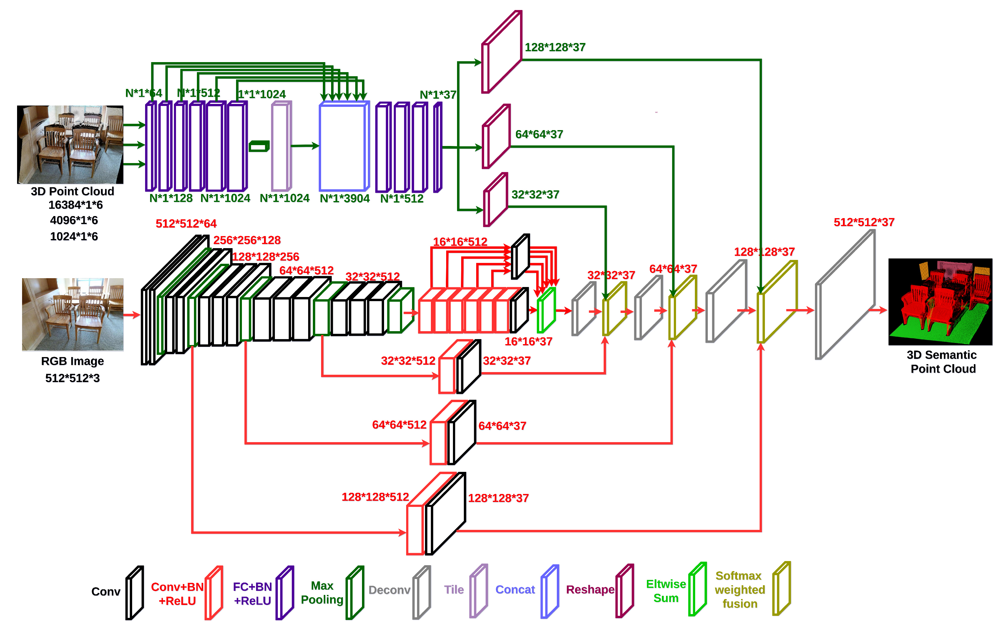
- A Pixel-Voxel network consuming the RGB image and point cloud is proposed, which can obtain global context information through PixelNet while preserving accurate local shape information through VoxelNet.
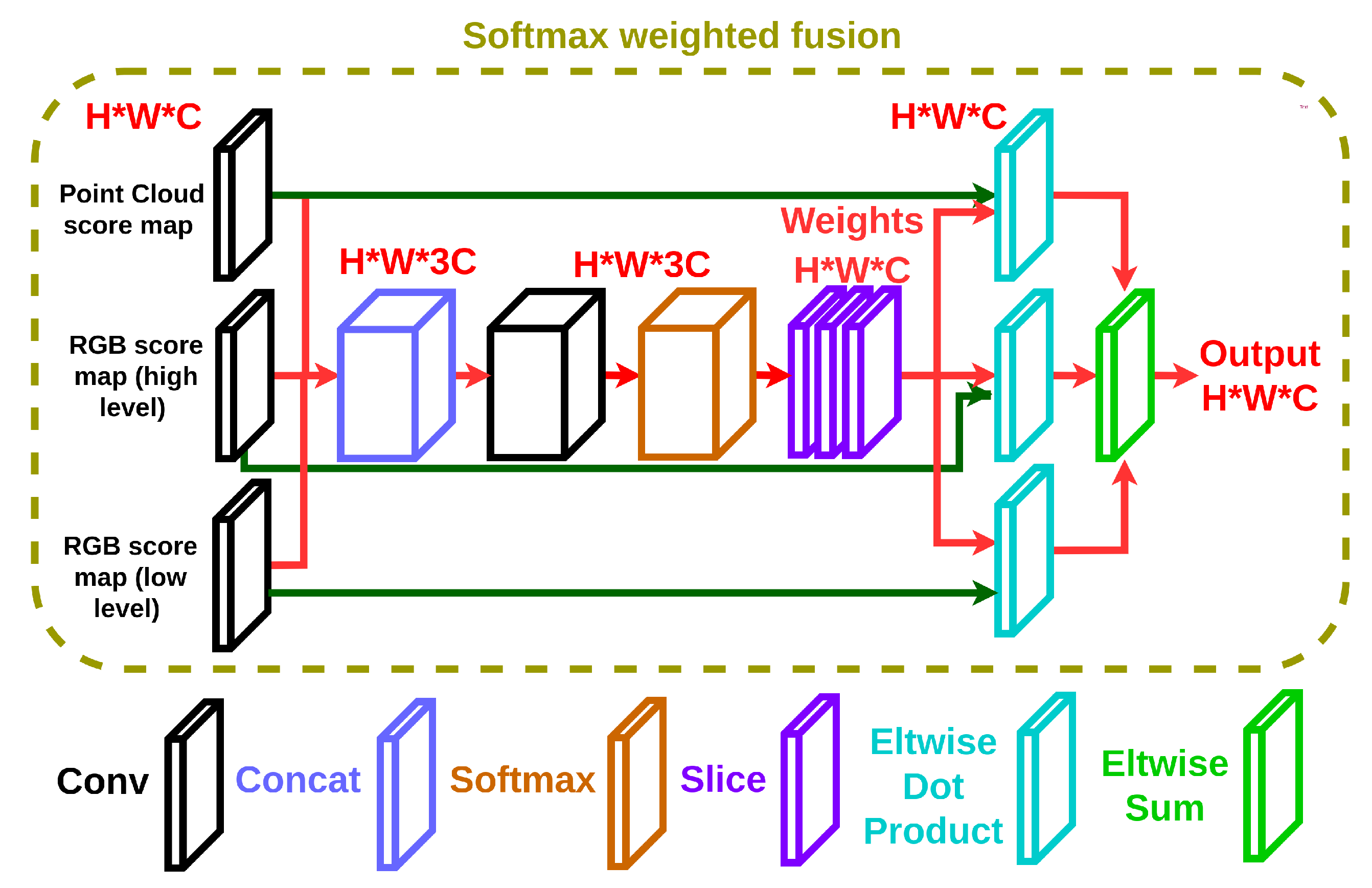
- A softmax weighted fusion stack is proposed to adaptively learn the varying contributions of different modalities. It can be inserted into a neural network to perform fusion-style end-to-end learning for arbitrary input modalities.
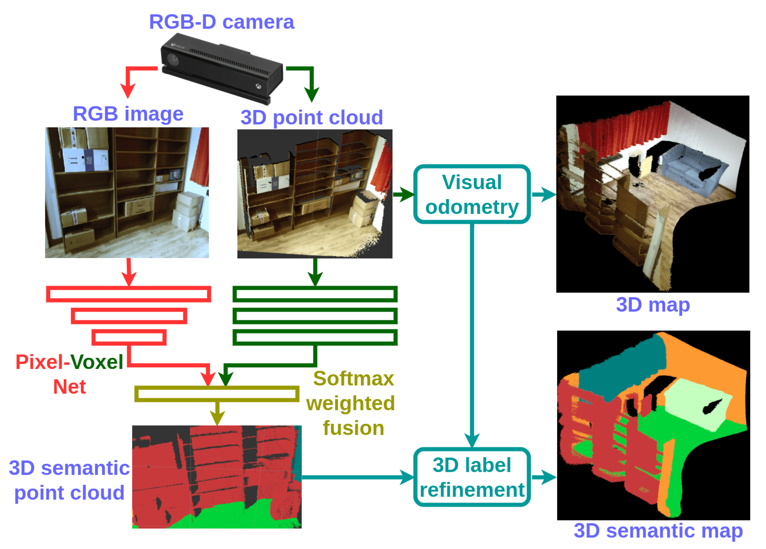
- A dense 3D semantic mapping system integrating a Pixel-Voxel network with RGB-D SLAM is developed. Its runtime can be boosted to around 13 Hz using an i7 eight-core PC with Titan X GPU, which is close to the requirements of real-time applications.
2. Related Work
2.1. Dense 3D Semantic Mapping
2.2. Fusion Style Semantic Segmentation
2.3. Discussion
3. Proposed Method
3.1. Overview
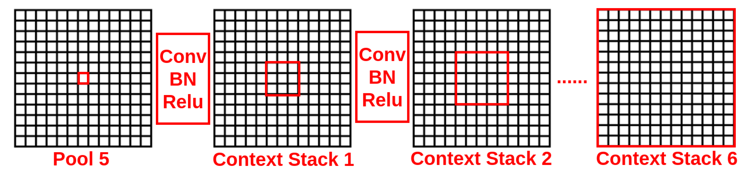
3.2. Pixel Neural Network
3.3. Voxel Neural Network
3.4. Softmax Weighed Fusion
3.5. Class-Weighted Loss Function
3.6. RGB-D Mapping and 3D Label Refinement
4. Experiments
4.1. Data Augmentation and Preprocessing
4.2. Network Training
4.3. Overall Performance
- Pixel accuracy:
- Mean accuracy:
- Mean IoU:
4.4. Dense RGB-D Semantic Mapping
5. Conclusions
Author Contributions
Funding
Acknowledgments
Conflicts of Interest
References
- Purkait, P.; Zhao, C.; Zach, C. SPP-Net: Deep Absolute Pose Regression with Synthetic Views. arXiv, 2018; arXiv:1712.03452. [Google Scholar]
- Zhao, C.; Sun, L.; Purkait, P.; Duckett, T.; Stolkin, R. Learning monocular visual odometry with dense 3D mapping from dense 3D flow. arXiv, 2018; arXiv:1803.02286. [Google Scholar]
- Zhao, C.; Mei, W.; Pan, W. Building a grid-semantic map for the navigation of service robots through human-robot interaction. Digit. Commun. Netw. 2015, 1, 253–266. [Google Scholar] [CrossRef]
- Zhao, C.; Hu, H.; Gu, D. Building a grid-point cloud-semantic map based on graph for the navigation of intelligent wheelchair. In Proceedings of the 2015 IEEE International Conference on Automation and Computing (ICAC), Glasgow, UK, 11–12 September 2015; pp. 1–7. [Google Scholar]
- Sun, L.; Yan, Z.; Molina, S.; Hanheide, M.; Duckett, T. 3DOF pedestrian trajectory prediction learned from long-term autonomous mobile robot deployment data. In Proceedings of the 2018 IEEE International Conference on Robotics and Automation (ICRA), Brisbane, Australia, 21–25 May 2018; pp. 5942–5948. [Google Scholar]
- Valiente, D.; Payá, L.; Jiménez, L.M.; Sebastián, J.M.; Reinoso, Ó. Visual Information Fusion through Bayesian Inference for Adaptive Probability-Oriented Feature Matching. Sensors 2018, 18, 2041. [Google Scholar] [CrossRef] [PubMed]
- Sun, L.; Zhao, C.; Duckett, T.; Stolkin, R. Weakly-supervised DCNN for RGB-D object recognition in real-world applications which lack large-scale annotated training data. arXiv, 2017; arXiv:1703.06370. [Google Scholar]
- Endres, F.; Hess, J.; Sturm, J.; Cremers, D.; Burgard, W. 3-D mapping with an RGB-D camera. Trans. Robot. 2014, 30, 177–187. [Google Scholar] [CrossRef]
- Newcombe, R.A.; Izadi, S.; Hilliges, O.; Molyneaux, D.; Kim, D.; Davison, A.J.; Kohi, P.; Shotton, J.; Hodges, S.; Fitzgibbon, A. KinectFusion: Real-time dense surface mapping and tracking. In Proceedings of the 2011 10th IEEE International Symposium on Mixed and Augmented Reality, Basel, Switzerland, 26–29 October 2011; pp. 127–136. [Google Scholar]
- Whelan, T.; Leutenegger, S.; Salas-Moreno, R.; Glocker, B.; Davison, A. ElasticFusion: Dense SLAM without a pose graph. In Proceedings of the Robotics: Scienceand Systems, Rome, Italy, 13–17 July 2015. [Google Scholar]
- Long, J.; Shelhamer, E.; Darrell, T. Fully convolutional networks for semantic segmentation. In Proceedings of the 2015 IEEE Conference on Computer Vision and Pattern Recognition (CVPR), Boston, MA, USA, 7–12 June 2015; pp. 3431–3440. [Google Scholar]
- Badrinarayanan, V.; Kendall, A.; Cipolla, R. Segnet: A deep convolutional encoder-decoder architecture for image segmentation. arXiv, 2015; arXiv:1511.00561. [Google Scholar]
- Chen, L.C.; Papandreou, G.; Kokkinos, I.; Murphy, K.; Yuille, A.L. Deeplab: Semantic image segmentation with deep convolutional nets, atrous convolution, and fully connected crfs. arXiv, 2016; arXiv:1606.00915. [Google Scholar]
- Hazirbas, C.; Ma, L.; Domokos, C.; Cremers, D. Fusenet: Incorporating depth into semantic segmentation via fusion-based cnn architecture. In Asian Conference on Computer Vision; Springer: Cham, Switzerland, 2016; pp. 213–228. [Google Scholar]
- Li, Z.; Gan, Y.; Liang, X.; Yu, Y.; Cheng, H.; Lin, L. LSTM-CF: Unifying context modeling and fusion with LSTMS for RGB-D scene labelling. In European Conference on Computer Vision; Springer: Cham, Switzerland, 2016; pp. 541–557. [Google Scholar]
- Cheng, Y.; Cai, R.; Li, Z.; Zhao, X.; Huang, K. Locality-Sensitive Deconvolution Networks with Gated Fusion for RGB-D Indoor Semantic Segmentation. In Proceedings of the 2017 IEEE Conference on Computer Vision and Pattern Recognition (CVPR), Honolulu, HI, USA, 21–26 July 2017; pp. 3029–3037. [Google Scholar]
- Lin, D.; Chen, G.; Cohen-Or, D.; Heng, P.A.; Huang, H. Cascaded Feature Network for Semantic Segmentation of RGB-D Images. In Proceedings of the 2017 IEEE International Conference on Computer Vision (ICCV), Venice, Italy, 22–29 October 2017; pp. 1311–1319. [Google Scholar]
- Qi, C.R.; Su, H.; Mo, K.; Guibas, L.J. Pointnet: Deep learning on point sets for 3d classification and segmentation. arXiv, 2016; arXiv:1612.00593. [Google Scholar]
- Qi, C.R.; Yi, L.; Su, H.; Guibas, L.J. PointNet++: Deep Hierarchical Feature Learning on Point Sets in a Metric Space. arXiv, 2017; arXiv:1706.02413. [Google Scholar]
- Salas-Moreno, R.F.; Newcombe, R.A.; Strasdat, H.; Kelly, P.H.; Davison, A.J. Slam++: Simultaneous localisation and mapping at the level of objects. In Proceedings of the 2013 IEEE Conference on Computer Vision and Pattern Recognition (CVPR), Sydney, Australia, 1–8 December 2013; pp. 1352–1359. [Google Scholar]
- Hermans, A.; Floros, G.; Leibe, B. Dense 3D semantic mapping of indoor scenes from RGB-D images. In Proceedings of the 2014 IEEE International Conference on Robotics and Automation (ICRA), Hong Kong, China, 31 May–7 June 2014; pp. 2631–2638. [Google Scholar]
- McCormac, J.; Handa, A.; Davison, A.; Leutenegger, S. Semanticfusion: Dense 3D semantic mapping with convolutional neural networks. In Proceedings of the 2017 IEEE International Conference on Robotics and Automation (ICRA), Singapore, 29 May–3 June 2017; pp. 4628–4635. [Google Scholar]
- Xiang, Y.; Fox, D. DA-RNN: Semantic Mapping with Data Associated Recurrent Neural Networks. arXiv, 2017; arXiv:1703.03098. [Google Scholar]
- Tateno, K.; Tombari, F.; Navab, N. When 2.5 D is not enough: Simultaneous reconstruction, segmentation and recognition on dense SLAM. In Proceedings of the 2016 IEEE International Conference on Robotics and Automation (ICRA), Stockholm, Sweden, 16–21 May 2016; pp. 2295–2302. [Google Scholar]
- Vineet, V.; Miksik, O.; Lidegaard, M.; Nießner, M.; Golodetz, S.; Prisacariu, V.A.; Kähler, O.; Murray, D.W.; Izadi, S.; Pérez, P.; et al. Incremental dense semantic stereo fusion for large-scale semantic scene reconstruction. In Proceedings of the 2015 IEEE International Conference on Robotics and Automation (ICRA), Seattle, WA, USA, 26–30 May 2015; pp. 75–82. [Google Scholar]
- Tateno, K.; Tombari, F.; Laina, I.; Navab, N. CNN-SLAM: Real-time dense monocular SLAM with learned depth prediction. arXiv, 2017; arXiv:1704.03489. [Google Scholar]
- Zhao, C.; Sun, L.; Stolkin, R. A fully end-to-end deep learning approach for real-time simultaneous 3D reconstruction and material recognition. In Proceedings of the 2017 IEEE International Conference on Advanced Robotics (ICAR), Hong Kong, China, 10–12 July 2017; pp. 75–82. [Google Scholar]
- Ma, L.; Stückler, J.; Kerl, C.; Cremers, D. Multi-view deep learning for consistent semantic mapping with RGB-D cameras. arXiv, 2017; arXiv:1703.08866. [Google Scholar]
- Mustafa, A.; Hilton, A. Semantically Coherent Co-segmentation and Reconstruction of Dynamic Scenes. In Proceedings of the 2017 Conference on Computer Vision and Pattern Recognition (CVPR), Honolulu, HI, USA, 21–26 July 2017. [Google Scholar]
- Noh, H.; Hong, S.; Han, B. Learning deconvolution network for semantic segmentation. In Proceedings of the 2015 IEEE International Conference on Computer Vision (ICCV), Las Condes, Chile, 11–18 December 2015; pp. 1520–1528. [Google Scholar]
- Krähenbühl, P.; Koltun, V. Efficient inference in fully connected crfs with gaussian edge potentials. In Advances in Neural Information Processing Systems; MIT Press: Cambridge, MA, USA, 2011; pp. 109–117. [Google Scholar]
- Zheng, S.; Jayasumana, S.; Romera-Paredes, B.; Vineet, V.; Su, Z.; Du, D.; Huang, C.; Torr, P.H. Conditional random fields as recurrent neural networks. In Proceedings of the 2015 IEEE International Conference on Computer Vision (ICCV), Las Condes, Chile, 11–18 December 2015; pp. 1529–1537. [Google Scholar]
- He, Y.; Chiu, W.C.; Keuper, M.; Fritz, M.; Campus, S.I. STD2P: RGBD Semantic Segmentation using Spatio-Temporal Data-Driven Pooling. In Proceedings of the 2017 Conference on Computer Vision and Pattern Recognition (CVPR), Honolulu, HI, USA, 21–26 July 2017. [Google Scholar]
- Shuai, B.; Liu, T.; Wang, G. Improving Fully Convolution Network for Semantic Segmentation. arXiv, 2016; arXiv:1611.08986. [Google Scholar]
- Shuai, B.; Zuo, Z.; Wang, B.; Wang, G. Dag-recurrent neural networks for scene labelling. In Proceedings of the 2016 Conference on Computer Vision and Pattern Recognition (CVPR), Las Vegas, NV, USA, 26 June–1 July 2016; pp. 3620–3629. [Google Scholar]
- Lin, G.; Shen, C.; Van Den Hengel, A.; Reid, I. Exploring context with deep structured models for semantic segmentation. IEEE Trans. Pattern Anal. Mach. Intell. 2017, 40, 1352–1366. [Google Scholar] [CrossRef] [PubMed]
- Lin, G.; Milan, A.; Shen, C.; Reid, I. Refinenet: Multi-path refinement networks for high-resolution semantic segmentation. In Proceedings of the 2017 Conference on Computer Vision and Pattern Recognition (CVPR), Honolulu, HI, USA, 21–26 July 2017. [Google Scholar]
- Handa, A.; Patraucean, V.; Badrinarayanan, V.; Stent, S.; Cipolla, R. Understanding real world indoor scenes with synthetic data. In Proceedings of the 2016 Conference on Computer Vision and Pattern Recognition (CVPR), Las Vegas, NV, USA, 26 June–1 July 2016; pp. 4077–4085. [Google Scholar]
- Eigen, D.; Fergus, R. Predicting depth, surface normals and semantic labels with a common multi-scale convolutional architecture. In Proceedings of the 2015 IEEE International Conference on Computer Vision (ICCV), Las Condes, Chile, 11–18 December 2015; pp. 2650–2658. [Google Scholar]
- Sun, L.; Yan, Z.; Zaganidis, A.; Zhao, C.; Duckett, T. Recurrent-OctoMap: Learning State-Based Map Refinement for Long-Term Semantic Mapping With 3-D-Lidar Data. IEEE Robot. Autom. Lett. 2018, 3, 3749–3756. [Google Scholar] [CrossRef]


| Methods | Pixel Acc. | Mean Acc. | Mean IoU |
|---|---|---|---|
| FCN [11] | 68.18% | 38.41% | 27.39% |
| DeconvNet [30] | 66.13% | 33.28% | 22.57% |
| SegNet [12] | 72.63% | 44.76% | 31.84% |
| DeepLab [13] | 71.90% | 42.21% | 32.08% |
| Context-CRF [36] | 78.4% | 53.4% | 42.3% |
| LSTM-CF [15] (RGB-D) | - | 48.1% | - |
| FuseNet [14] (RGB-D) | 76.27% | 48.30% | 37.29% |
| LS-DeconvNets (RGB-D) [16] | - | 58.00% | - |
| RefineNet-Res101 [37] | 80.4% | 57.8% | 45.7% |
| RefineNet-Res152 [37] | 80.6% | 58.5% | 45.9% |
| CFN (VGG-16, RGB-D) [17] | - | - | 42.5% |
| CFN (RefineNet-152, RGB-D) [17] | - | - | 48.1% |
| Pixel Net (VGG-16) | 77.25% | 49.33% | 38.26% |
| Pixel Net (ResNet101) | 78.30% | 54.22% | 41.73% |
| Pixel-Voxel Net (VGG-16, without fusion) | 77.82% | 53.86% | 41.33% |
| Pixel-Voxel Net (ResNet101, without fusion) | 78.76% | 56.81% | 43.59% |
| Pixel-Voxel Net (VGG-16) | 78.14% | 54.79% | 42.11% |
| Pixel-Voxel Net (ResNet101) | 79.04% | 57.65% | 44.24% |
| Methods | Pixel Acc. | Mean Acc. | Mean IoU |
|---|---|---|---|
| Hermans et al. [21] (RGB-D) † | 54.3% | 48.0% | - |
| SemanticFusion [22] † | 67.9% | 59.2% | - |
| SceneNet [38] | 67.2% | 52.5% | - |
| Eigen et al. [39] (RGB-D) | 75.4% | 66.9% | 52.6% |
| FuseNet [14] (RGB-D) | 75.8% | 66.2% | 54.2% |
| Ma et al. [28] (RGB-D) † | 79.13% | 70.59% | 59.07% |
| Pixel Net (VGG-16) † | 80.74% | 70.23% | 55.92% |
| Pixel Net (ResNet101) † | 81.63% | 72.18% | 57.78% |
| Pixel-Voxel Net (VGG-16, without fusion) † | 81.50% | 72.25% | 57.69% |
| Pixel-Voxel Net (ResNet101, without fusion) † | 82.22% | 73.64% | 58.71% |
| Pixel-Voxel Net (VGG-16) † | 81.85% | 73.21% | 58.54% |
| Pixel-Voxel Net (ResNet101) † | 82.53% | 74.43% | 59.30% |
| Category | Wall | Floor | Cabinet | Bed | Chair | Sofa | Table | Door | Window | Bookshelf | Picture | Counter | Blinds |
| SegNet [12] | 83.42% | 93.43% | 63.37% | 73.18% | 75.92% | 59.57% | 64.18% | 52.50% | 57.51% | 42.05% | 56.17% | 37.66% | 40.29% |
| LSTM-CF [15] | 74.9% | 82.3% | 47.3% | 62.1% | 67.7% | 55.5% | 57.8% | 45.6% | 52.8% | 43.1% | 56.7% | 39.4% | 48.6% |
| FuseNet [14] | 90.20% | 94.91% | 61.81% | 77.10% | 78.62% | 66.49% | 65.44% | 46.51% | 62.44% | 34.94% | 67.39% | 40.37% | 43.48% |
| LS-DeconvNets [16] | 91.9% | 94.7% | 61.6% | 82.2% | 87.5% | 62.8% | 68.3% | 47.9% | 68.0% | 48.4% | 69.1% | 49.4% | 51.3% |
| PVNet (VGG16) | 90.28% | 93.21% | 66.87% | 75.31% | 85.45% | 67.37% | 64.81% | 58.62% | 63.58% | 54.54% | 64.76% | 51.87% | 59.23% |
| PVNet (ResNet101) | 89.19% | 94.94% | 69.36% | 79.11% | 85.70% | 66.09% | 60.59% | 62.22% | 66.59% | 58.34% | 66.39% | 50.56% | 53.65% |
| PVNet (VGG16) | 76.07% | 87.20% | 50.66% | 68.23% | 64.98% | 54.17% | 46.07% | 44.83% | 46.50% | 41.31% | 48.94% | 41.19% | 39.95% |
| PVNet (ResNet101) | 77.41% | 87.78% | 53.44% | 71.16% | 66.76% | 54.61% | 44.46% | 45.19% | 48.23% | 41.79% | 46.78% | 41.39% | 35.95% |
| Category | Desk | Shelves | Curtain | Dresser | Pillow | Mirror | Floor_Mat | Clothes | Ceiling | Books | Fridge | TV | Paper |
| SegNet [12] | 11.92% | 11.45% | 66.56% | 52.73% | 43.80% | 26.30% | 0.00% | 34.31% | 74.11% | 53.77% | 29.85% | 33.76% | 22.73% |
| LSTM-CF [15] | 37.3% | 9.6% | 63.4% | 35.0% | 45.8% | 44.5% | 0.0% | 28.4% | 68.0% | 47.9% | 61.5% | 52.1% | 36.4% |
| FuseNet [14] | 25.63% | 20.28% | 65.94% | 44.03% | 54.28% | 52.47% | 0.00% | 25.89% | 84.77% | 45.23% | 34.52% | 34.83% | 24.08% |
| LS-DeconvNets [16] | 35.0% | 24.0% | 68.7% | 60.5% | 66.5% | 57.6% | 0.00% | 44.4% | 88.8% | 61.5% | 51.4% | 71.7% | 37.3% |
| PVNet (VGG16) | 32.05% | 23.09% | 62.49% | 62.13% | 54.97% | 50.60% | 0.59% | 35.35% | 57.78% | 41.75% | 55.43% | 67.60% | 35.34% |
| PVNet (ResNet101) | 32.49% | 27.37% | 68.33% | 69.41% | 56.96% | 57.94% | 0.00% | 36.45% | 68.77% | 42.02% | 63.05% | 72.47% | 38.11% |
| PVNet (VGG16) | 26.05% | 12.05% | 50.52% | 47.43% | 36.35% | 36.44% | 0.59% | 20.56% | 53.61% | 28.04% | 41.23% | 57.36% | 24.13% |
| PVNet (ResNet101) | 25.30% | 16.86% | 53.09% | 50.83% | 38.16% | 42.29% | 0.00% | 22.28% | 63.39% | 29.21% | 48.47% | 60.46% | 25.20% |
| Category | Towel | Shower_Curtain | Box | Whiteboard | Person | Night_Stand | Toilet | Sink | Lamp | Bathtub | Bag | Mean | - |
| SegNet [12] | 19.83% | 0.03% | 23.14% | 60.25% | 27.27% | 29.88% | 76.00% | 58.10% | 35.27% | 48.86% | 16.76% | 31.84% | - |
| LSTM-CF [15] | 36.7% | 0.0% | 38.1% | 48.1% | 72.6% | 36.4% | 68.8% | 67.9% | 58.0% | 65.6% | 23.6% | 48.1% | - |
| FuseNet [14] | 21.05% | 8.82% | 21.94% | 57.45% | 19.06% | 37.15% | 76.77% | 68.11% | 49.31% | 73.23% | 12.62% | 48.30% | - |
| LS-DeconvNets [16] | 51.4% | 2.9% | 46.0% | 54.2% | 49.1% | 44.6% | 82.2% | 74.2% | 64.7% | 77.0% | 47.6% | 58.0% | - |
| PVNet (VGG16) | 41.12% | 4.59% | 40.33% | 66.56% | 60.51% | 33.21% | 80.62% | 69.07% | 60.35% | 67.78% | 28.17% | 54.79% | - |
| PVNet (ResNet101) | 48.81% | 0.00% | 42.15% | 74.22% | 69.40% | 38.16% | 80.23% | 68.20% | 61.80% | 76.16% | 37.63% | 57.65% | - |
| PVNet (VGG16) | 30.53% | 4.00% | 24.81% | 51.10% | 48.57% | 20.89% | 66.31% | 48.82% | 43.50% | 55.90% | 19.37% | 42.11% | - |
| PVNet (ResNet101) | 36.85% | 0.00% | 26.77% | 54.88% | 54.77% | 21.52% | 66.43% | 53.15% | 43.00% | 65.00% | 23.90% | 44.24% | - |
| Category | Bed | Books | Ceiling | Chair | Floor | Furniture | Objects | Painting | Sofa | Table | TV | Wall | Window | Mean |
|---|---|---|---|---|---|---|---|---|---|---|---|---|---|---|
| Hermans et al. [21] † | 68.4% | 45.4% | 83.4% | 41.9% | 91.5% | 37.1% | 8.6% | 35.8% | 28.5% | 27.7% | 38.4% | 71.8% | 46.1% | 48.0% |
| SemanticFusion [22] † | 62.0% | 58.4% | 43.3% | 59.5% | 92.7% | 64.4% | 58.3% | 65.8% | 48.7% | 34.3% | 34.3% | 86.3% | 62.3% | 59.2% |
| PVNet (VGG16) † | 74.85% | 49.93% | 82.18% | 78.67% | 98.82% | 63.43% | 52.57% | 63.06% | 70.41% | 74.48% | 73.48% | 94.85% | 74.98% | 73.21% |
| PVNet (ResNet101) † | 73.85% | 59.60% | 76.14% | 81.99% | 98.33% | 58.82% | 59.19% | 66.27% | 64.07% | 78.41% | 79.67% | 94.53% | 76.66% | 74.43% |
| PVNet (VGG16) † | 64.17% | 33.34% | 64.05% | 64.25% | 90.39% | 49.27% | 40.95% | 45.17% | 54.78% | 62.83% | 52.31% | 80.62% | 58.87% | 58.54% |
| PVNet (ResNet101) † | 63.09% | 38.35% | 61.16% | 68.58% | 89.66% | 48.07% | 44.34% | 50.39% | 50.89% | 63.48% | 49.97% | 81.51% | 61.40% | 59.30% |
| Network on the Different Sizes of Data | Inference Runtime | |
|---|---|---|
| Full Size | Half Size | |
| PVNet (VGG-16) | 0.176s | 0.075s |
| PVNet (ResNet101) | 0.310s | 0.111s |
| Network on the Half Size Data | SUN RGB-D | NYU V2 | ||||
|---|---|---|---|---|---|---|
| △ Pixel acc. | △ Mean acc. | △ Mean IoU | △ Pixel acc. | △ Mean acc. | △ Mean IoU | |
| PVNet (VGG-16) | −1.35% | −1.87% | −1.59% | −1.08% | −0.62% | −1.53% |
| PVNet (ResNet101) | −1.16% | −2.34% | −1.94% | −1.41% | −0.84% | −1.96% |
© 2018 by the authors. Licensee MDPI, Basel, Switzerland. This article is an open access article distributed under the terms and conditions of the Creative Commons Attribution (CC BY) license (http://creativecommons.org/licenses/by/4.0/).
Share and Cite
Zhao, C.; Sun, L.; Purkait, P.; Duckett, T.; Stolkin, R. Dense RGB-D Semantic Mapping with Pixel-Voxel Neural Network. Sensors 2018, 18, 3099. https://doi.org/10.3390/s18093099
Zhao C, Sun L, Purkait P, Duckett T, Stolkin R. Dense RGB-D Semantic Mapping with Pixel-Voxel Neural Network. Sensors. 2018; 18(9):3099. https://doi.org/10.3390/s18093099
Chicago/Turabian StyleZhao, Cheng, Li Sun, Pulak Purkait, Tom Duckett, and Rustam Stolkin. 2018. "Dense RGB-D Semantic Mapping with Pixel-Voxel Neural Network" Sensors 18, no. 9: 3099. https://doi.org/10.3390/s18093099
APA StyleZhao, C., Sun, L., Purkait, P., Duckett, T., & Stolkin, R. (2018). Dense RGB-D Semantic Mapping with Pixel-Voxel Neural Network. Sensors, 18(9), 3099. https://doi.org/10.3390/s18093099