WiFi Indoor Localization with CSI Fingerprinting-Based Random Forest

Abstract
1. Introduction
2. CSI Data Analysis
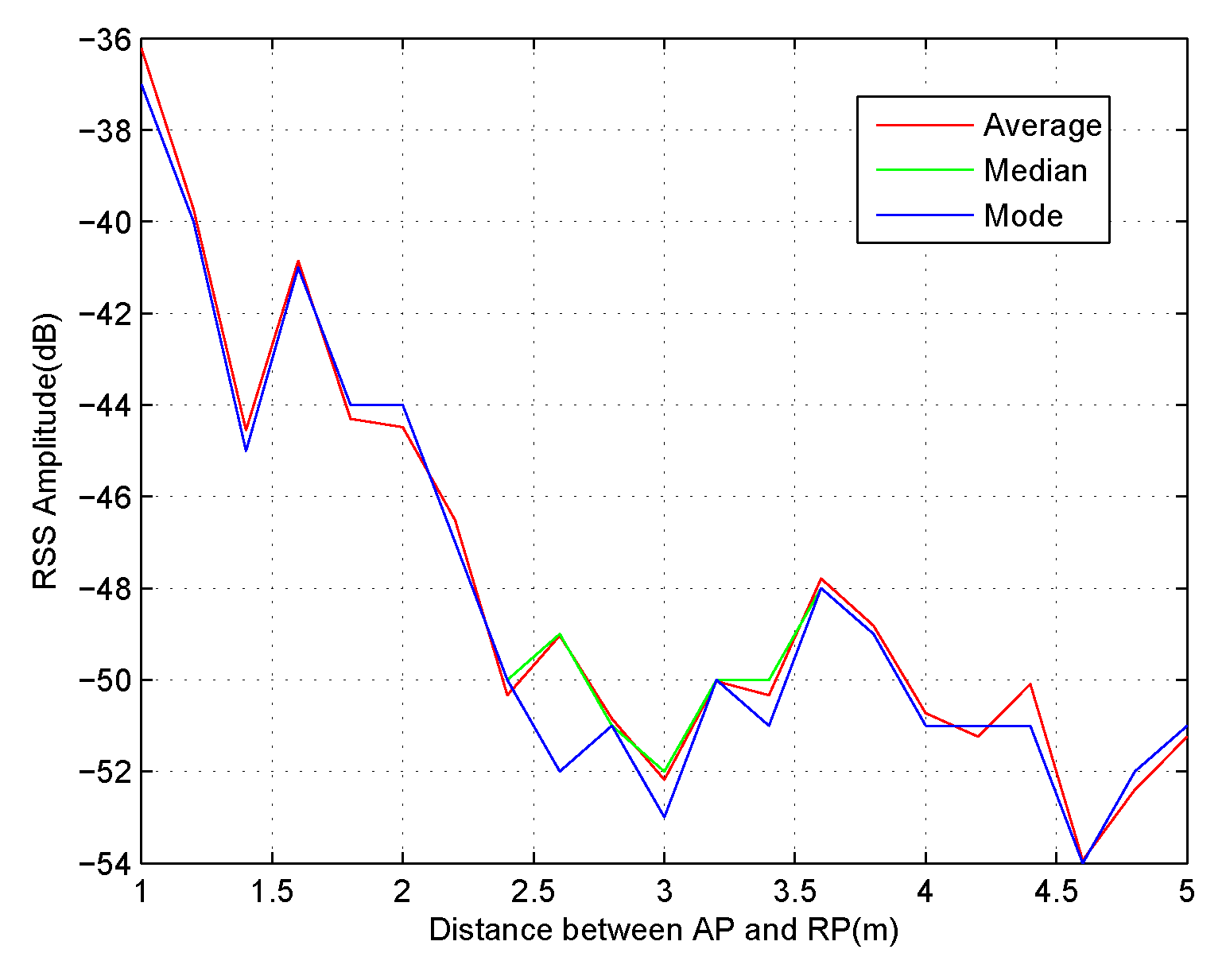
2.1. Location Correlation
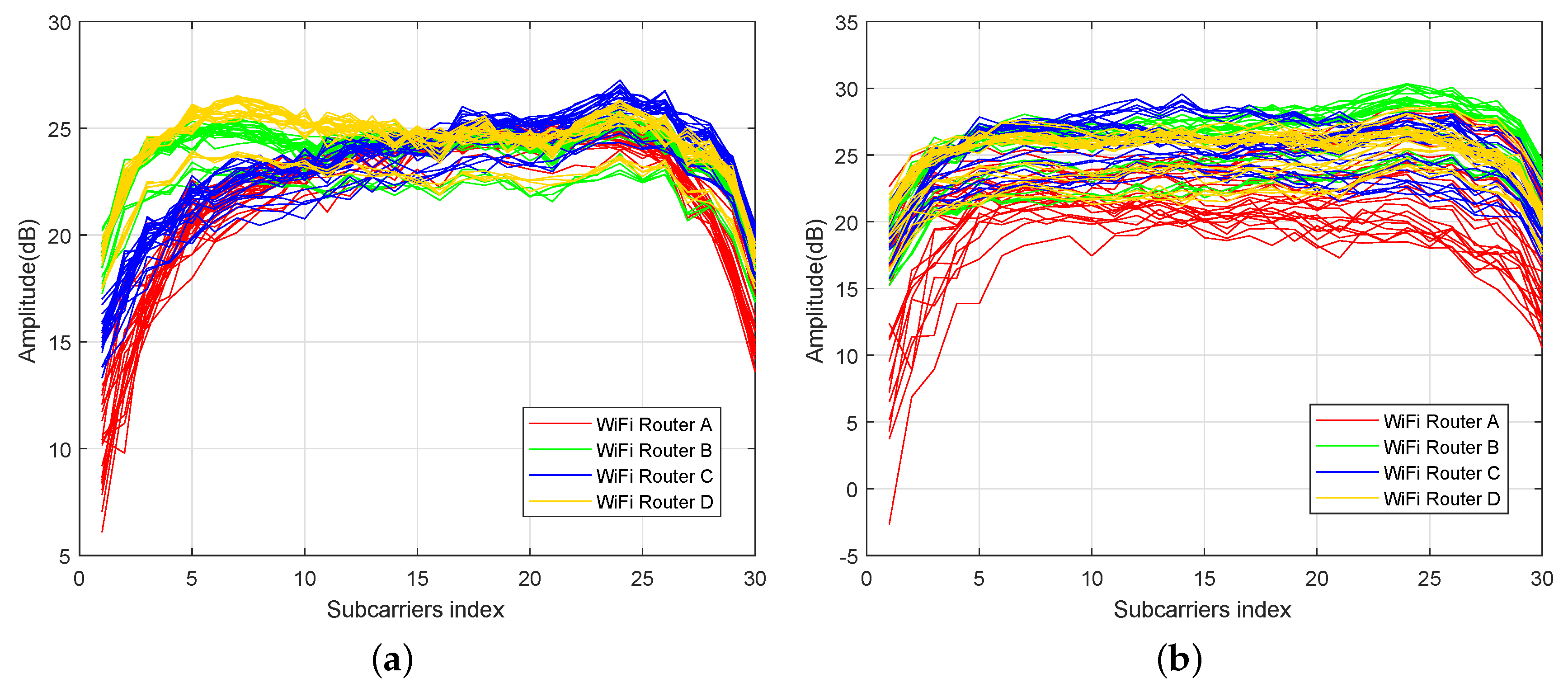
2.2. Time-Varying
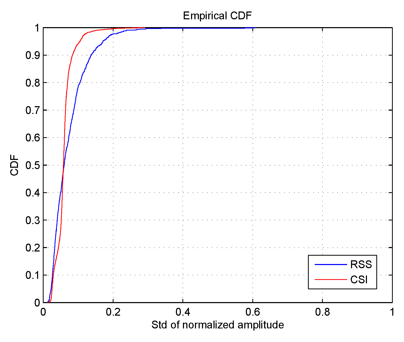
2.3. Incompleteness
3. RFFP System
3.1. Proposed Algorithm
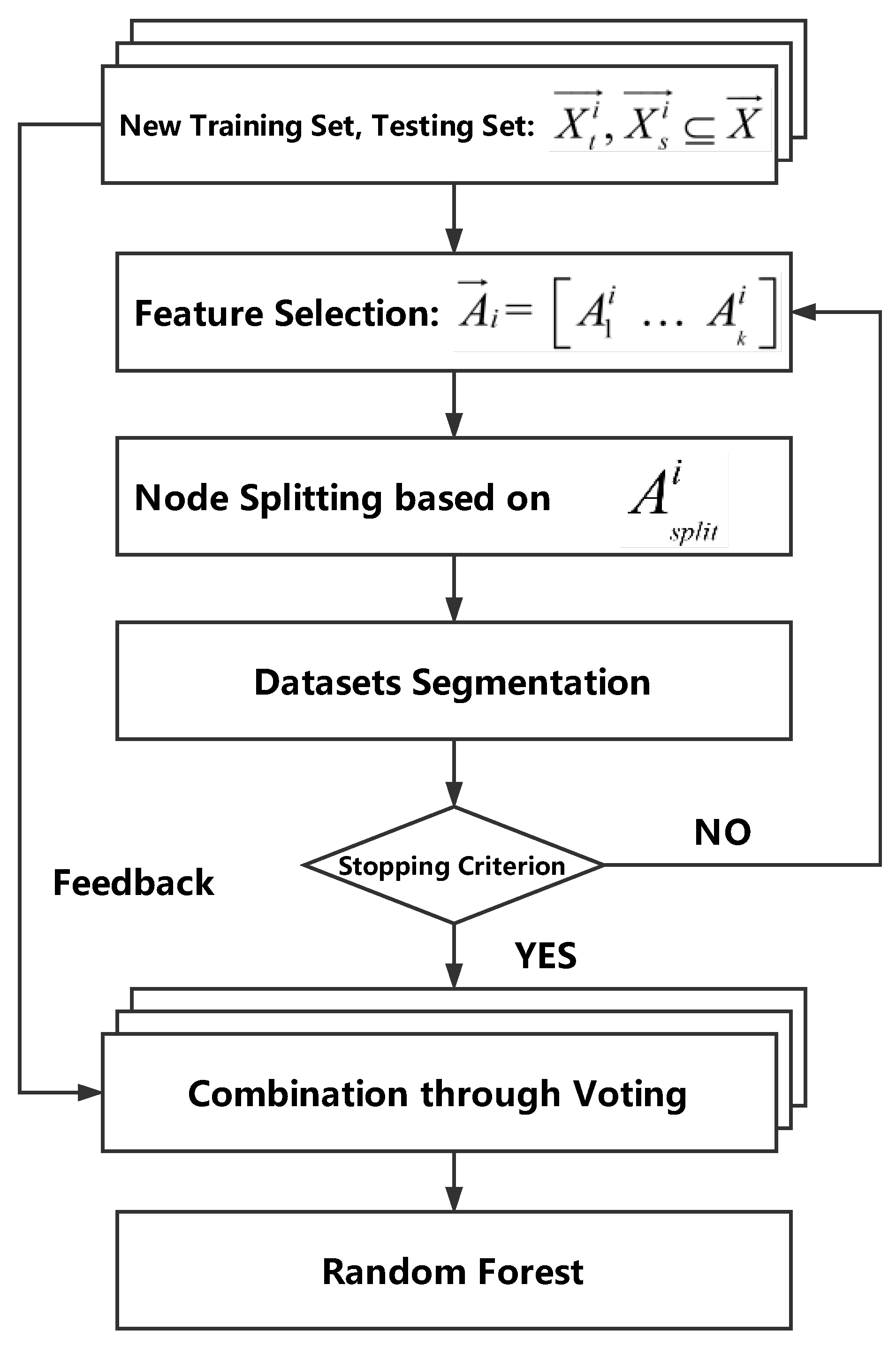
3.1.1. Feedback Decision Tree
| Algorithm 1. Building phase of the Feedback Decision Tree |
 |
3.1.2. Random Forest
| Algorithm 2. Random Forest construction with Feedback Decision Tree |
 |
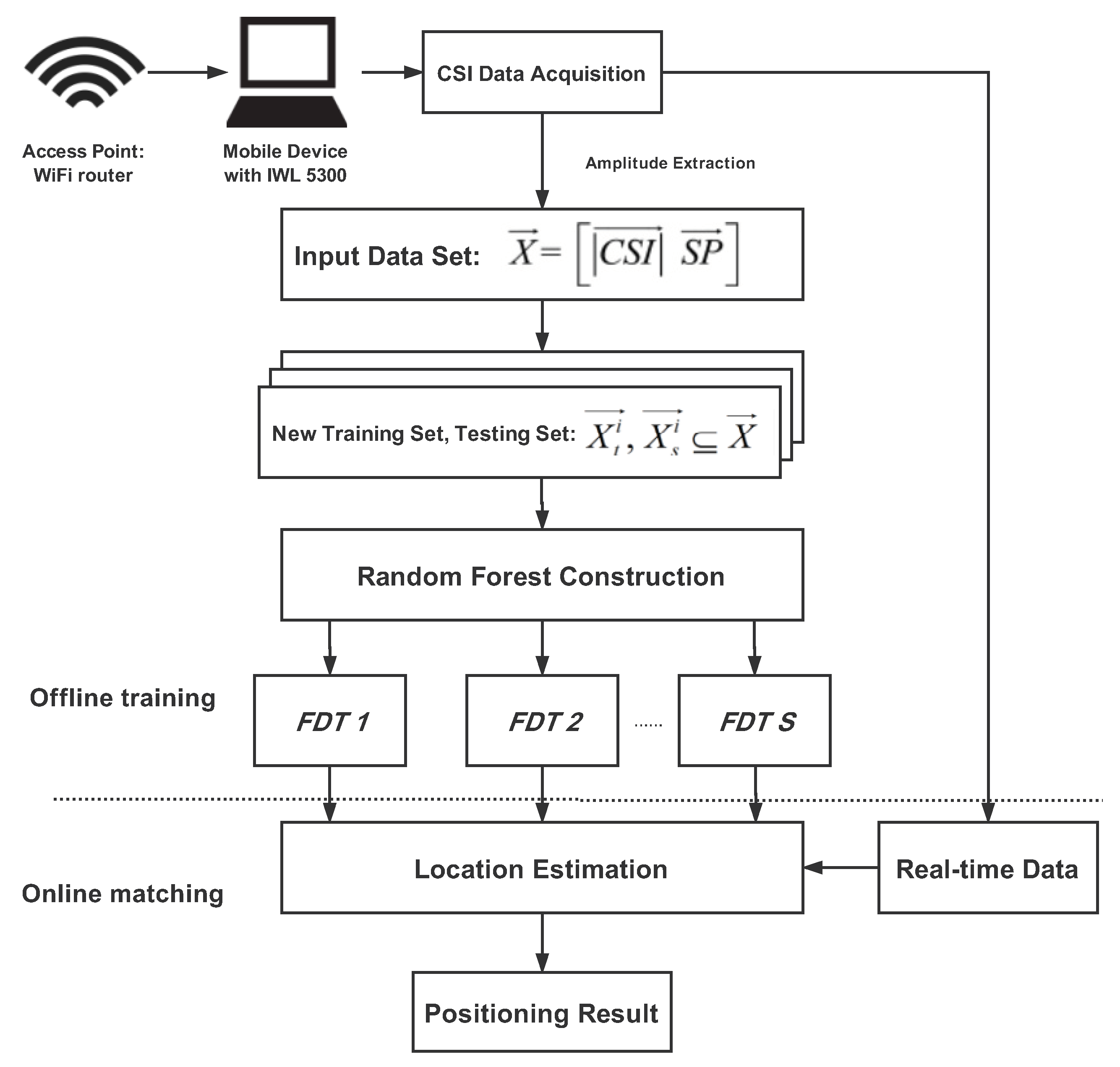
3.2. RFFP System Architecture
4. Experiments and Discussion
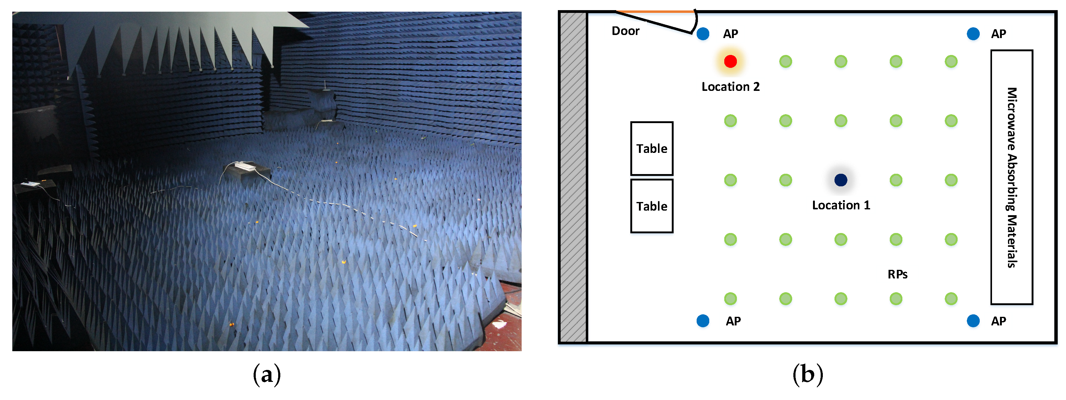
4.1. Experiment Setting
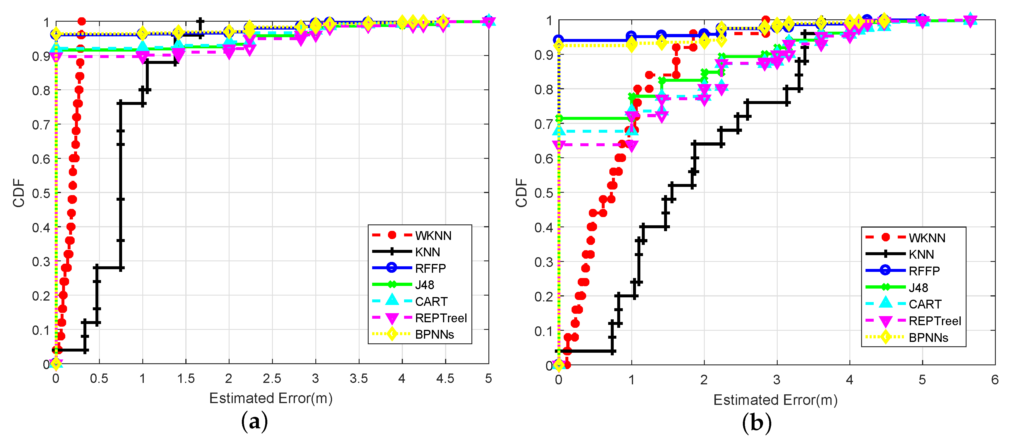
4.2. Localization Precision
4.2.1. Impact of Wireless Channel Circumstances
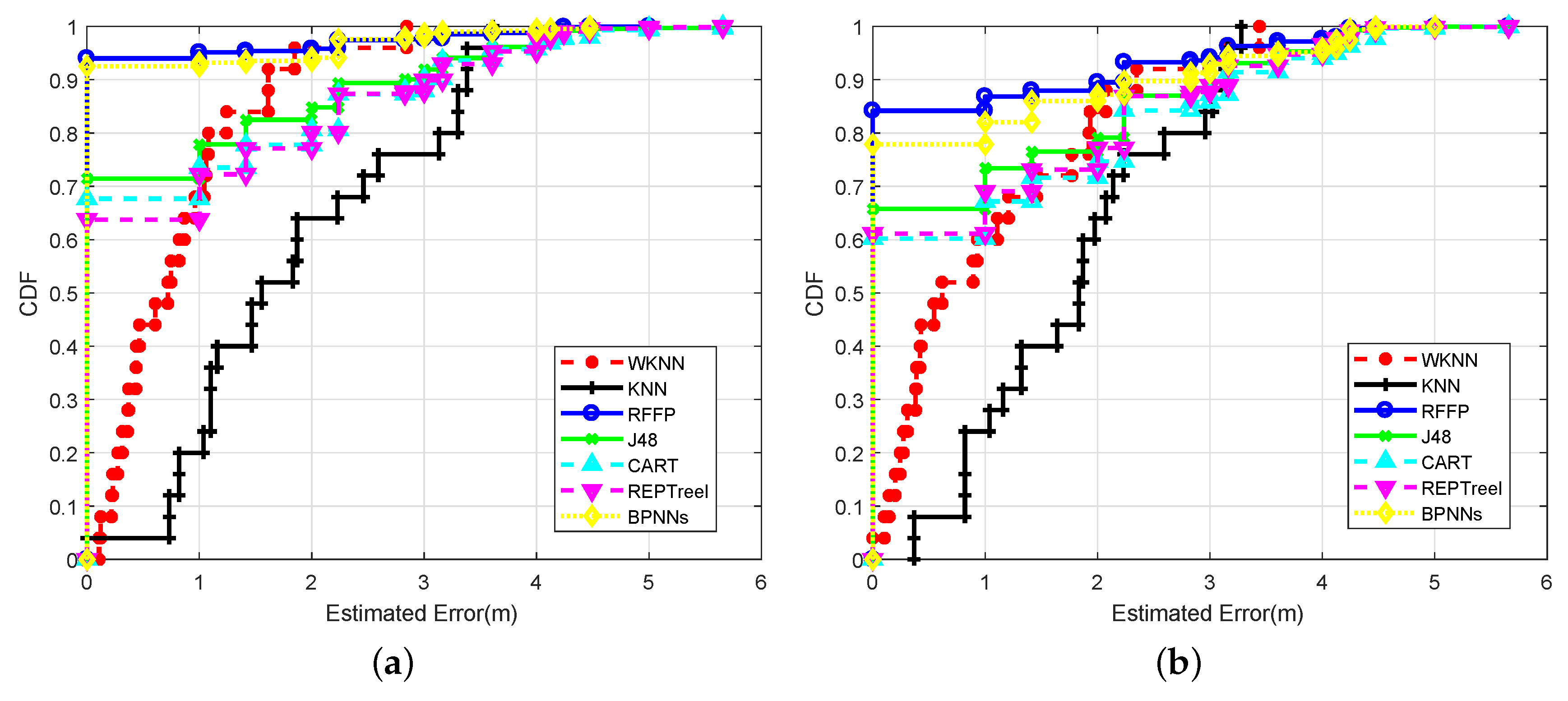
4.2.2. Impact of Channel Environment
4.2.3. Impact of Input Datasets
4.3. Effects of Different Hyperparameters
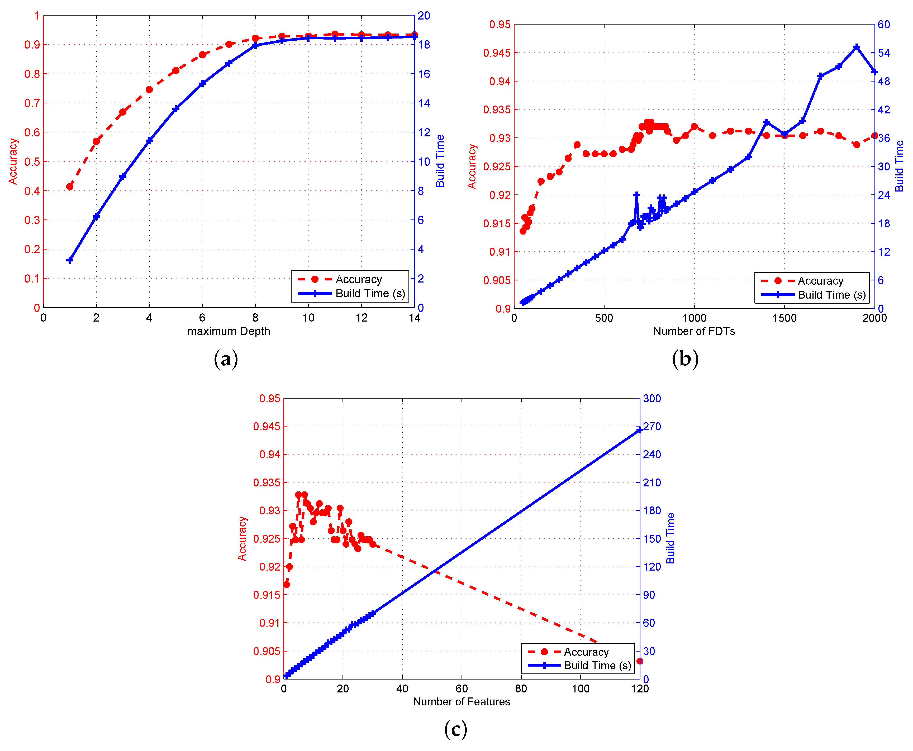
4.3.1. Impact of Maximum Depths of FDT
4.3.2. Impact of the Number of FDTs in RFFP
4.3.3. Impact of the Number of Features
5. Conclusions
Author Contributions
Funding
Conflicts of Interest
References
- Buchli, B.; Sutton, F.; Beutel, J. GPS-Equipped Wireless Sensor Network Node for High-Accuracy Positioning Applications. In European Conference on Wireless Sensor Networks; Springer: New York, NY, USA, 2012; pp. 179–195. [Google Scholar]
- Zou, H.; Lu, X.; Jiang, H.; Xie, L. A fast and precise indoor localization algorithm based on an online sequential extreme learning machine. Sensors 2015, 15, 1804–1824. [Google Scholar] [CrossRef] [PubMed]
- Liu, H.; Darabi, H.; Banerjee, P.; Liu, J. Survey of wireless indoor positioning techniques and systems. IEEE Trans. Syst. Man Cybern. C Appl. Rev. 2007, 37, 1067–1080. [Google Scholar] [CrossRef]
- Gu, Y.; Lo, A.; Niemegeers, I. A survey of indoor positioning systems for wireless personal networks. IEEE Commun. Surv. Tutor. 2009, 11, 13–32. [Google Scholar] [CrossRef]
- Deak, G.; Curran, K.; Condell, J. A survey of active and passive indoor localisation systems. Comput. Commun. 2012, 35, 1939–1954. [Google Scholar] [CrossRef]
- Zhang, D.; Yang, L.T.; Chen, M.; Zhao, S.; Guo, M.; Zhang, Y. Real-time locating systems using active rfid for internet of things. IEEE Syst. J. 2017, 10, 1226–1235. [Google Scholar] [CrossRef]
- Ni, L.M.; Liu, Y.; Lau, Y.C.; Patil, A.P. Landmarc: Indoor location sensing using active rfid. Wirel. Netw. 2004, 10, 701–710. [Google Scholar] [CrossRef]
- Pahlavan, K.; Li, X.; Makela, J.P. Indoor geolocation science and technology. IEEE Commun. Mag. 2002, 40, 112–118. [Google Scholar] [CrossRef]
- Yuan, Z.; Yang, J.; You, L.; Qi, L.; Naser, E.S. Smartphone-based indoor localization with bluetooth low energy beacons. Sensors 2016, 16, 596. [Google Scholar] [CrossRef]
- Senger, C. Modeling and simulation of ultra wideband indoor localization systems in soft non-line-of-sight. J. Am. Chem. Soc. 2012, 117, 474–477. [Google Scholar]
- Yoon, P.K.; Zihajehzadeh, S.; Kang, B.S.; Park, E.J. Robust biomechanical model-based 3D indoor localization and tracking method using UWB and IMU. IEEE Sens. J. 2017, 17, 1084–1096. [Google Scholar] [CrossRef]
- Li, Z.; Yang, T.; Li, G.; Li, J.; Zhang, Y. Geodetic coordinate calculation based on monocular vision on UAV platform. In Proceedings of the International Conference on Signal Processing (ICSP), Chengdu, China, 6–10 November 2016. [Google Scholar]
- Li, D.; Zhang, B.; Li, C. A Feature-Scaling-Based k-Nearest Neighbor Algorithm for Indoor Positioning Systems. IEEE Internet Things J. 2016, 3, 590–597. [Google Scholar] [CrossRef]
- Farjow, W.; Chehri, A.; Hussein, M.; Fernando, X. Support Vector Machines for indoor sensor localization. In Proceedings of the Wireless Communications and NETWORKING Conference, Cancun, Mexico, 28–31 March 2011. [Google Scholar]
- Wu, Z.L.; Li, C.H.; Ng, J.K.Y.; Leung, K.R.P.H. Location Estimation via Support Vector Regression. IEEE Trans. Mob. Comput. 2007, 6, 311–321. [Google Scholar] [CrossRef]
- Hansen, L.K.; Salamon, P. Neural network ensembles. IEEE Trans. Pattern Anal. Mach. Intell. 1990, 12, 993–1001. [Google Scholar] [CrossRef]
- Breiman, L. Random forests. Mach. Learn. 2001, 45, 5–32. [Google Scholar] [CrossRef]
- Zhang, P.B.; Yang, Z.H. A novel AdaBoost framework with robust threshold and structural optimization. IEEE Trans. Cybern. 2018, 48, 64–76. [Google Scholar] [CrossRef] [PubMed]
- Song, C.J.; Wang, J. WLAN Fingerprint Indoor Positioning Strategy Based on Implicit Crowdsourcing and Semi-Supervised Learning. ISPRS Int. J. Geo-Inf. 2017, 6, 356. [Google Scholar] [CrossRef]
- Bernas, M.; Placzek, B. Fully Connected Neural Networks Ensemble with Signal Strength Clustering for Indoor Localization in Wireless Sensor Networks. Int. J. Distrib. Sens. Netw. 2015, 11, 403242. [Google Scholar] [CrossRef]
- Ding, W.; Yang, F.; Liu, S.; Wang, X.; Song, J. Nonorthogonal Time-Frequency Training-Sequence-Based CSI Acquisition for MIMO Systems. IEEE Trans. Veh. Technol. 2016, 65, 5714–5719. [Google Scholar] [CrossRef]
- Drakshayini, M.N.; Singh, A.V. A review on reconfigurable orthogonal frequency division multiplexing (OFDM) system for wireless communication. In Proceedings of the International Conference on Applied and Theoretical Computing and Communication Technology, Bangalore, India, 21–23 July 2016. [Google Scholar]
- Wu, K.; Xiao, J.; Yi, Y.; Chen, D.; Luo, X.; Ni, L.M. Csi-based indoor localization. IEEE Trans. Parallel Distrib. Syst. 2013, 24, 1300–1309. [Google Scholar] [CrossRef]
- Fang, S.H.; Chang, W.H.; Yu, T.; Shih, H.C.; Wang, C. Channel State Reconstruction Using Multilevel Discrete Wavelet Transform for Improved Fingerprinting-Based Indoor Localization. IEEE Sens. J. 2016, 16, 7787–7791. [Google Scholar] [CrossRef]
- Li, J.; Li, Y.; Ji, X. A novel method of Wi-Fi indoor localization based on channel state information. In Proceedings of the International Conference on Wireless Communications & Signal Processing, Yangzhou, China, 13–15 October 2016. [Google Scholar]
- Li, X.; Cai, X.; Hei, Y.; Yuan, R. NLOS identification and mitigation based on channel state information for indoor WiFi localisation. IET Commun. 2017, 11, 531–537. [Google Scholar] [CrossRef]
- Berkvens, R.; Peremans, H.; Weyn, M. Conditional Entropy and Location Error in Indoor Localization Using Probabilistic Wi-Fi Fingerprinting. Sensors 2016, 16, 1636. [Google Scholar] [CrossRef] [PubMed]
- Torressospedra, J.; Moreira, A. Analysis of Sources of Large Positioning Errors in Deterministic Fingerprinting. Sensors 2017, 17, 2736. [Google Scholar] [CrossRef] [PubMed]
- Lindner, C.; Bromiley, P.A.; Ionita, M.C.; Cootes, T.F. Robust and Accurate Shape Model Matching Using Random Forest Regression-Voting. IEEE Trans. Pattern Anal. Mach. Intell. 2015, 37, 1862–1874. [Google Scholar] [CrossRef] [PubMed]
- Ni, B.; Yan, S.; Wang, M.; Kassim, A.A.; Tian, Q. High-Order Local Spatial Context Modeling by Spatialized Random Forest. IEEE Trans. Image Process. 2013, 22, 739–751. [Google Scholar] [PubMed]
- Wang, X.; Gao, L.; Mao, S.; Pandey, S. Csi-based fingerprinting for indoor localization: A deep learning approach. IEEE Trans. Veh. Technol. 2017, 66, 763–776. [Google Scholar] [CrossRef]
- Yang, Y.; Chen, W. Taiga: Performance Optimization of the C4.5 Decision Tree Construction Algorithm. Tsinghua Sci. Technol. 2016, 21, 415–425. [Google Scholar] [CrossRef]
- Sun, J.; Zhong, G.; Dong, J.; Saeeda, H.; Zhang, Q. Cooperative profit random forests with application in ocean front recognition. IEEE Access 2017, 5, 1398–1408. [Google Scholar] [CrossRef]
- Liu, X.; Song, M.; Tao, D.; Liu, Z.; Zhang, L.; Chen, C.; Bu, J. Random forest construction with robust semisupervised node splitting. IEEE Trans. Image Process. 2015, 24, 471–483. [Google Scholar] [CrossRef] [PubMed]
- Quinlan, J.R. Induction of decision trees. Mach. Learn. 1986, 1, 81–106. [Google Scholar] [CrossRef]
- Gaddam, S.R.; Phoha, V.V.; Balagani, K.S. K-Means+ID3: A Novel Method for Supervised Anomaly Detection by Cascading K-Means Clustering and ID3 Decision Tree Learning Methods. IEEE Trans. Knowl. Data Eng. 2007, 19, 345–354. [Google Scholar] [CrossRef]
- Breiman, L.; Friedman, J.H.; Olshen, R.A.; Stone, C.J. Classification and Regression Trees; Routledge: Abingdon-on-Thames, UK, 1984. [Google Scholar]
- Zhao, S.; Liu, Y.; Jiang, J.; Cheng, W.; Zhou, M.; Li, M.; Yuan, R. Extraction of mangrove in Hainan Dongzhai Harbor based on CART decision tree. In Proceedings of the 2014 22nd International Conference on Geoinformatics, Kaohsiung, Taiwan, 25–27 June 2014. [Google Scholar]
- Zhao, P.; Fu, Y.F.; Zheng, L.G.; Feng, X.Z.; Satyanarayana, B. Cart-based Land Use/cover Classification of Remote Sensing Images. J. Remote Sens. 2005, 9, 708–716. [Google Scholar]
- Deng, H.W.; Zhang, J.G. Gene selection for classification of microarray data based on the Bayes error. BMC Bioinform. 2007, 8, 370. [Google Scholar]
- Shah, S.A.A.; Aziz, W.; Arif, M.; Nadeem, M.S.A. Decision Trees Based Classification of Cardiotocograms Using Bagging Approach. In Proceedings of the Frontiers of Information Technology, Islamabad, Pakistan, 14–16 December 2015. [Google Scholar]
- Breiman, L. The Little Bootstrap and other Methods for Dimensionality Selection in Regression: X-Fixed Prediction Error. J. Am. Stat. Assoc. 1992, 87, 738–754. [Google Scholar] [CrossRef]
- Heath, D.; Kasif, S.; Salzberg, S. Induction of Oblique Decision Trees. J. Artif. Intell. Res. 1993, 2, 1–32. [Google Scholar]
- Dinh-Van, N.; Nashashibi, F.; Thanh-Huong, N.; Castelli, E. Indoor Intelligent Vehicle localization using WiFi received signal strength indicator. In Proceedings of the IEEE Mtt-S International Conference on Microwaves for Intelligent Mobility, Nagoya, Japan, 19–21 March 2017; pp. 33–36. [Google Scholar]


| Algorithm | KNN | WKNN | RFFP | ||
|---|---|---|---|---|---|
| InPut Data | RSSI | CSI | RSSI | CSI | CSI |
| MAE in chamber (m) | 1.7085 | 0.7608 | 1.1255 | 0.1767 | 0.1033 |
| MAE in office, LOS (m) | 2.8724 | 1.8421 | 2.1812 | 0.8164 | 0.1708 |
| MAE in office, NLOS (m) | 2.9463 | 1.7782 | 2.3071 | 1.0517 | 0.4033 |
| Algorithm | J48 | CART | REPTree | Ensemble of BPNNs | RFFP |
|---|---|---|---|---|---|
| Accuracy (chamber) | 91.64% | 92.08% | 89.68% | 96.36% | 96.04% |
| Accuracy (office, LOS) | 71.44% | 67.68% | 63.76% | 92.52% | 93.12% |
| Accuracy (office, NLOS) | 65.74% | 60.20% | 61.13% | 77.88% | 84.18% |
| Number of APs | Accuracy | OOBE | MAE (m) | TP Rate | FP Rate | Precision | F-Measure | Build Time (s) |
|---|---|---|---|---|---|---|---|---|
| 1 | 75.28% | 13.44% | 0.5864 | 0.753 | 0.01 | 0.758 | 0.751 | 27.42 |
| 2 | 89.92% | 9.76% | 0.2548 | 0.899 | 0.004 | 0.902 | 0.899 | 28.63 |
| 3 | 92.48% | 7.2% | 0.1930 | 0.925 | 0.03 | 0.927 | 0.925 | 29.5 |
| 4 | 93.12% | 6.56% | 0.1708 | 0.931 | 0.03 | 0.934 | 0.931 | 30.3 |
© 2018 by the authors. Licensee MDPI, Basel, Switzerland. This article is an open access article distributed under the terms and conditions of the Creative Commons Attribution (CC BY) license (http://creativecommons.org/licenses/by/4.0/).
Share and Cite
Wang, Y.; Xiu, C.; Zhang, X.; Yang, D. WiFi Indoor Localization with CSI Fingerprinting-Based Random Forest. Sensors 2018, 18, 2869. https://doi.org/10.3390/s18092869
Wang Y, Xiu C, Zhang X, Yang D. WiFi Indoor Localization with CSI Fingerprinting-Based Random Forest. Sensors. 2018; 18(9):2869. https://doi.org/10.3390/s18092869
Chicago/Turabian StyleWang, Yanzhao, Chundi Xiu, Xuanli Zhang, and Dongkai Yang. 2018. "WiFi Indoor Localization with CSI Fingerprinting-Based Random Forest" Sensors 18, no. 9: 2869. https://doi.org/10.3390/s18092869
APA StyleWang, Y., Xiu, C., Zhang, X., & Yang, D. (2018). WiFi Indoor Localization with CSI Fingerprinting-Based Random Forest. Sensors, 18(9), 2869. https://doi.org/10.3390/s18092869