Three-Dimensional Terahertz Coded-Aperture Imaging Based on Back Projection

 ,
,
Abstract
:1. Introduction
2. Imaging Method
2.1. Traditional TCAI
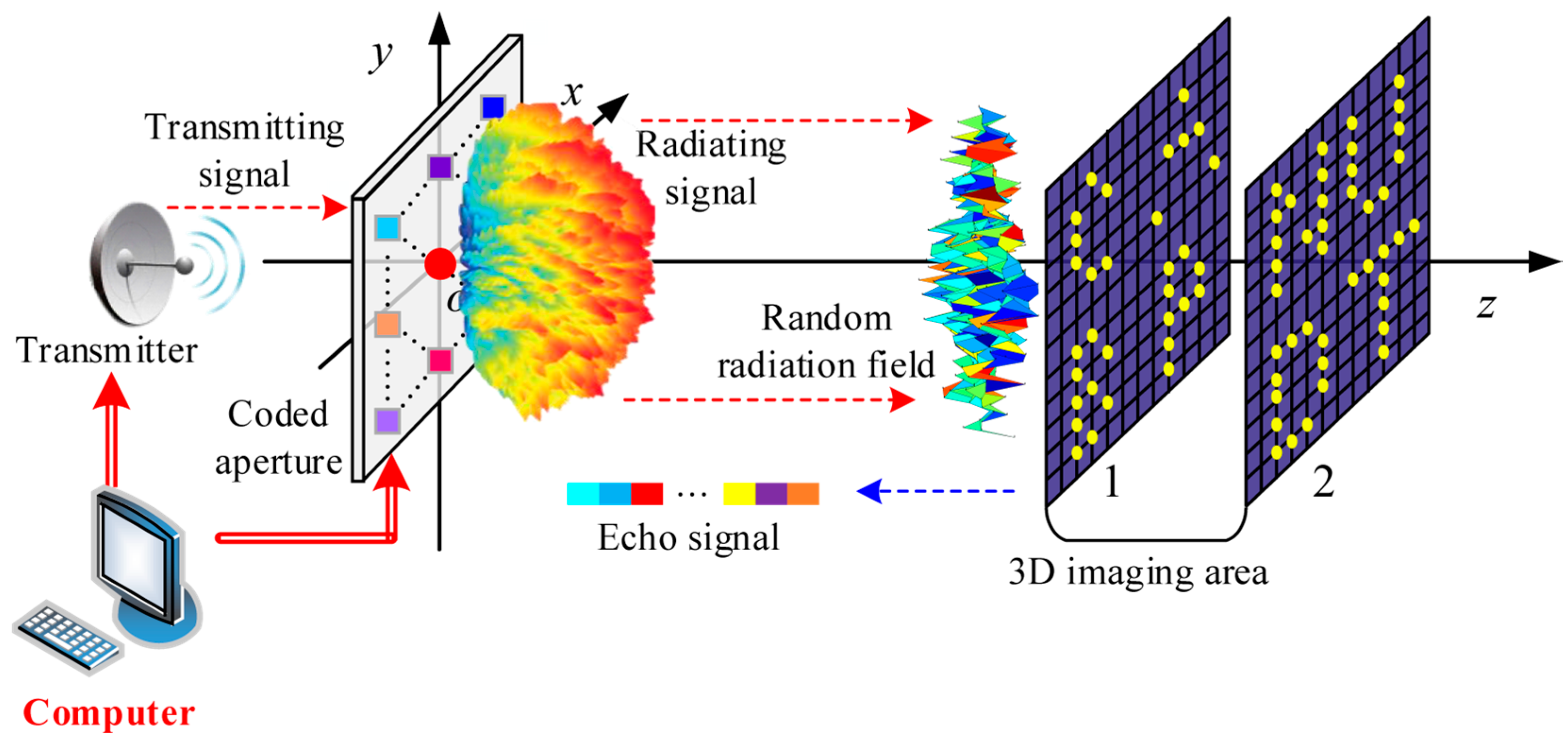
2.1.1. Signal Propagation
2.1.2. Imaging Model
2.2. GM-Based TCAI
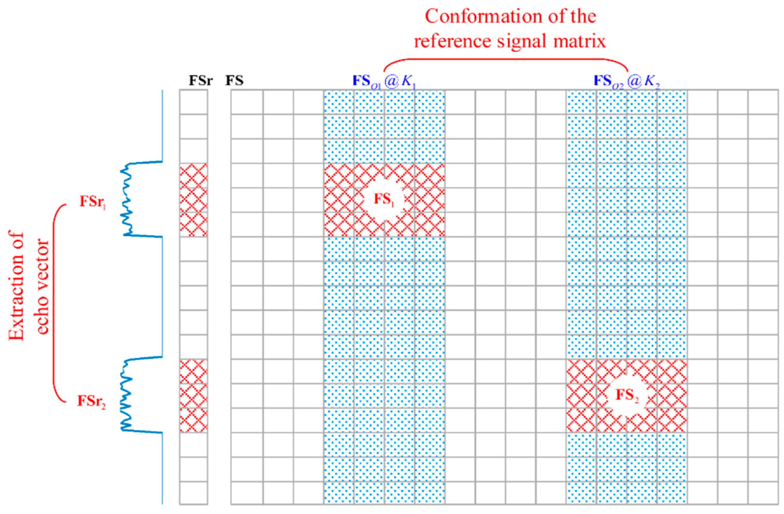
2.2.1. EV Extraction of GM-TCAI
2.2.2. RSM Conformation of GM-TCAI
2.2.3. Imaging Model of GM-TCAI
2.3. BP-Based TCAI
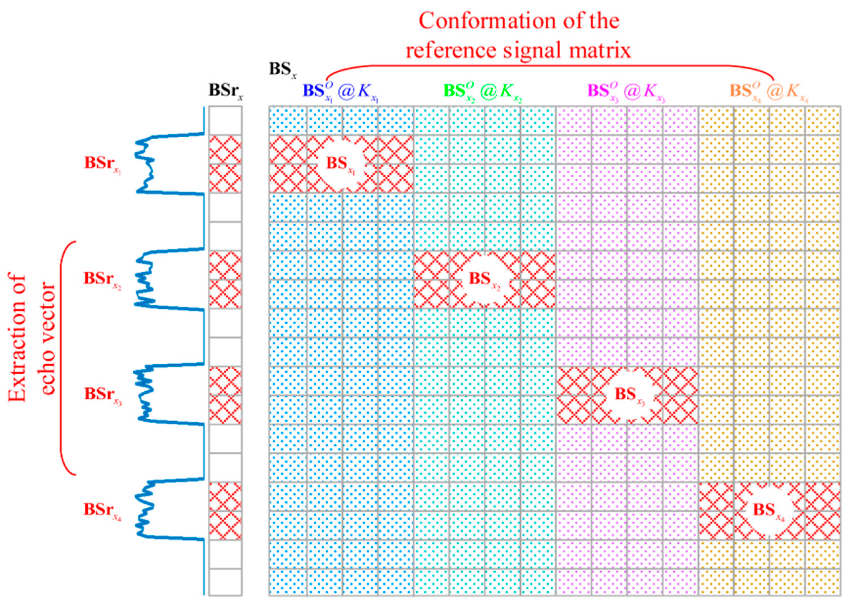
2.3.1. EV Extraction of BP-TCAI
2.3.2. RSM Conformation of BP-TCAI
2.3.3. Imaging Model of BP-TCAI
2.4. Comparisons of Computational Complexity
3. Experimental Results
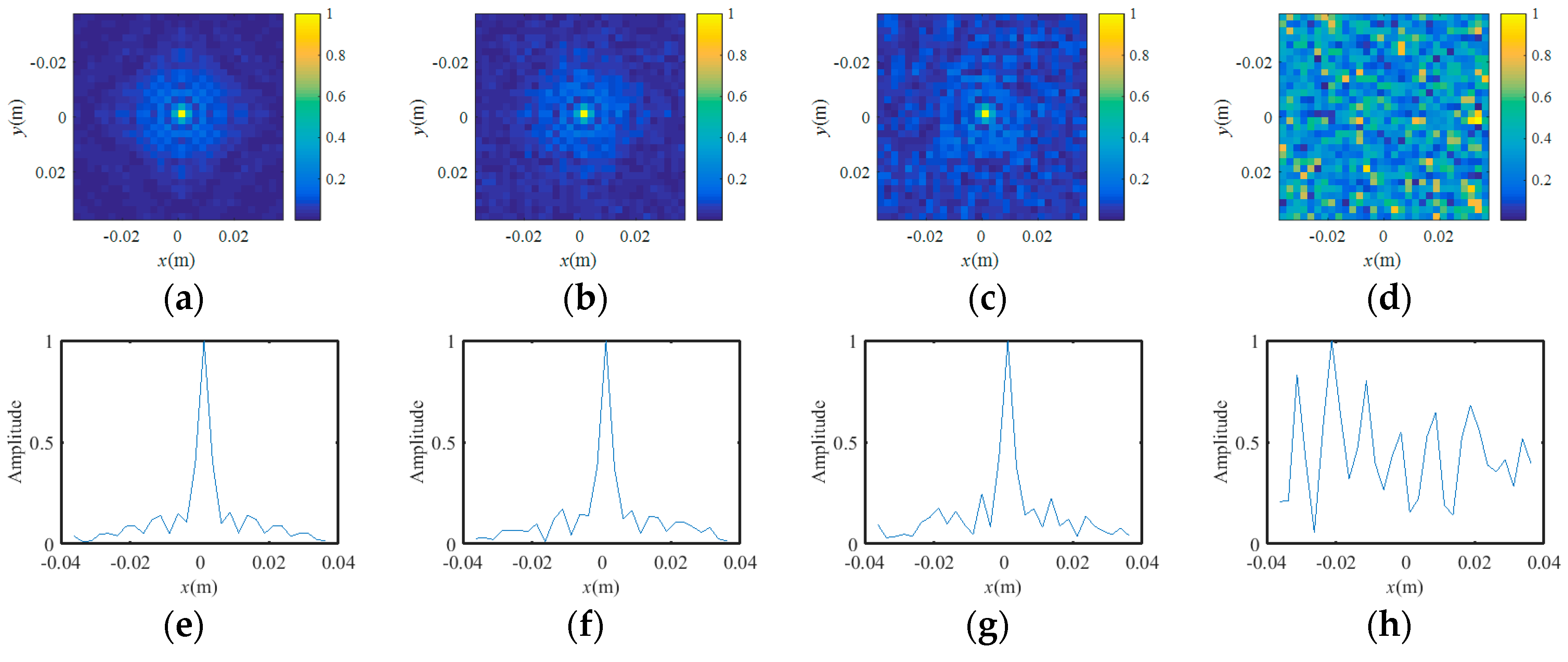
3.1. PSF Analysis
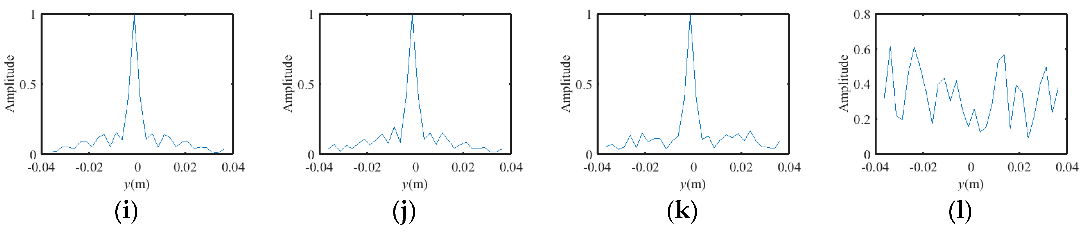
3.2. Range Profile Analysis
3.3. Projection Results of BP
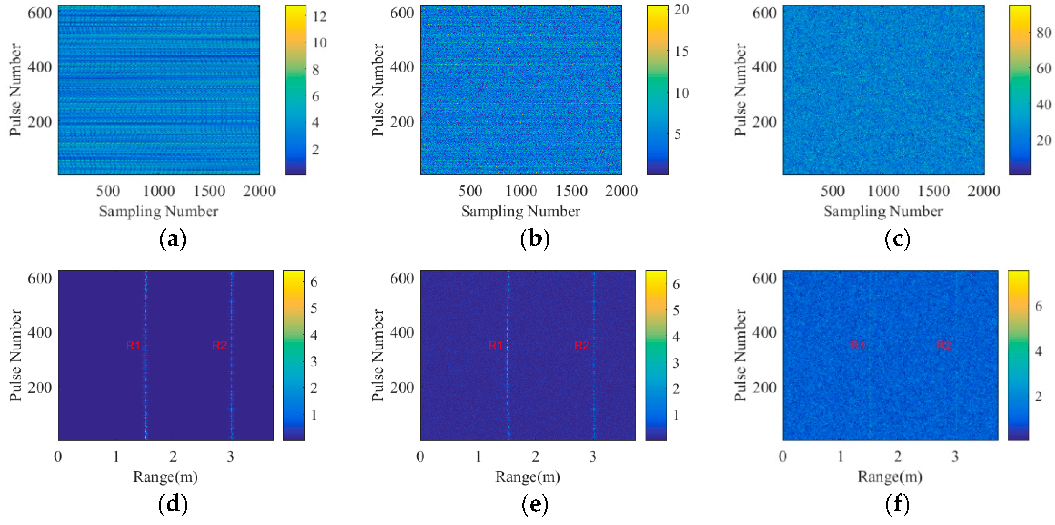
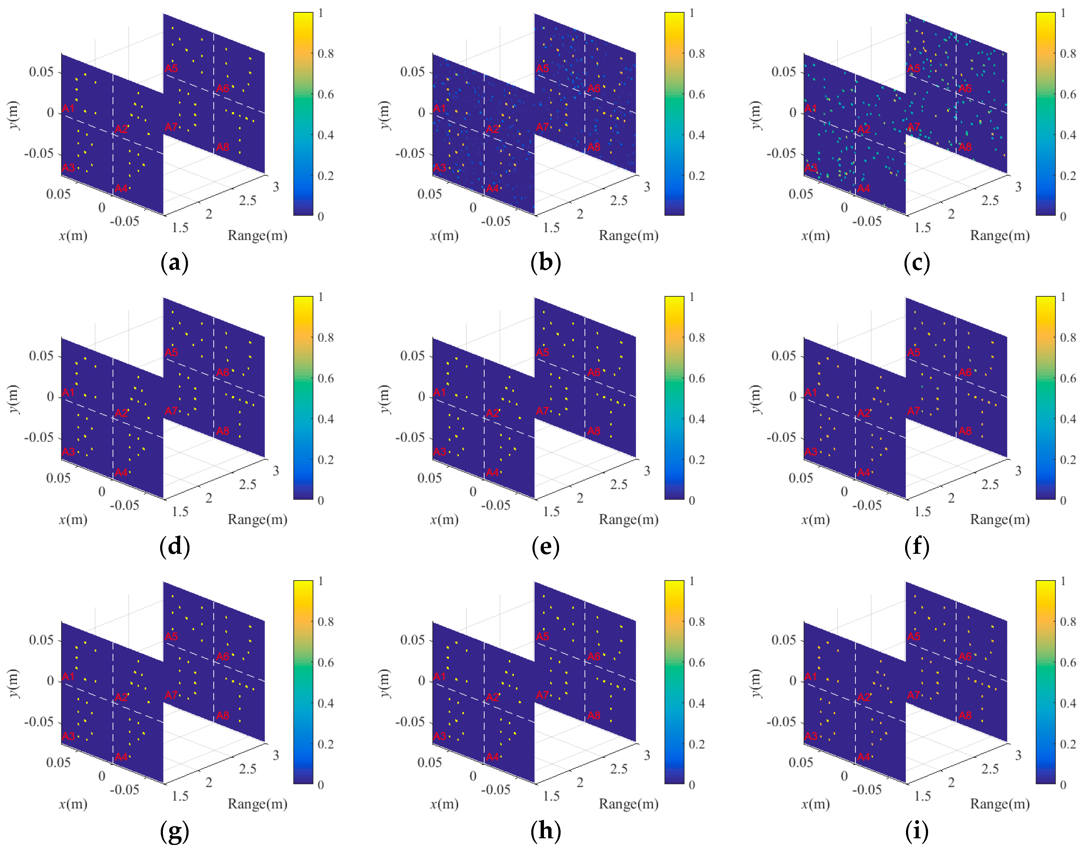
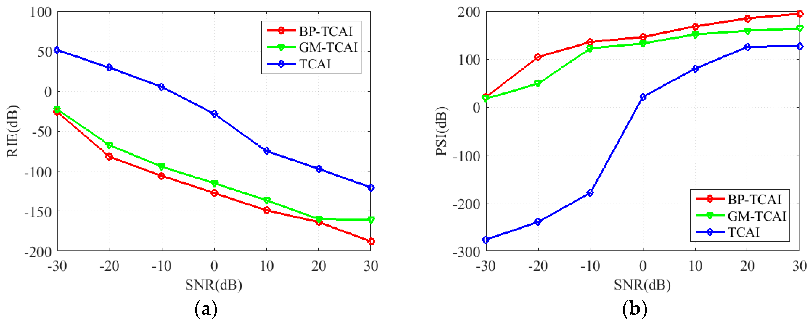
3.4. Imaging Results Analysis
4. Conclusions
Author Contributions
Funding
Conflicts of Interest
References
- Watts, C.M.; Shrekenhamer, D.; Montoya, J.; Lipworth, G.; Hunt, J.; Sleasman, T.; Krishna, S.; Smith, D.R.; Padilla, W.J. Terahertz compressive imaging with metamaterial spatial light modulators. Nat. Photonics 2014, 8, 605–609. [Google Scholar] [CrossRef]
- Li, Y.B.; Li, L.L.; Xu, B.B.; Wu, W.; Wu, R.Y.; Wan, X.; Cheng, Q.; Cui, T.J. Transmission-type 2-bit programmable metasurface for single-sensor and single-frequency microwave imaging. Sci. Rep. 2016, 6, 23731. [Google Scholar] [CrossRef] [PubMed]
- Gollub, J.N.; Yurduseven, O.; Trofatter, K.P.; Arnitz, D.; F Imani, M.; Sleasman, T.; Boyarsky, M.; Rose, A.; Pedross-Engel, A.; Odabasi, H.; et al. Large metasurface aperture for millimeter wave computational imaging at the human-scale. Sci. Rep. 2017, 7, 42650. [Google Scholar] [CrossRef] [PubMed]
- Liu, Z.; Tan, S.; Wu, J.; Li, E.; Shen, X.; Han, S. Spectral camera based on ghost imaging via sparsity constraints. Sci. Rep. 2016, 6, 25718. [Google Scholar] [CrossRef] [PubMed]
- Yu, H.; Lu, R.; Han, S.; Xie, H.; Du, G.; Xiao, T.; Zhu, D. Fourier-transform ghost imaging with hard X rays. Phys. Rev. Lett. 2016, 117, 113901. [Google Scholar] [CrossRef] [PubMed]
- Li, D.; Li, X.; Qin, Y.; Cheng, Y.; Wang, H. Radar Coincidence Imaging: An Instantaneous Imaging Technique with Stochastic Signals. IEEE Trans. Geosci. Remote Sens. 2014, 52, 2261–2277. [Google Scholar]
- Li, D.; Li, X.; Qin, Y.; Cheng, Y.; Wang, H. Radar Coincidence Imaging under Grid Mismatch. ISRN Signal Process. 2016, 2014, 987803. [Google Scholar] [CrossRef]
- Tribe, W.R.; Taday, P.F.; Kemp, M.C. Hidden object detection: Security applications of terahertz technology. Proc. SPIE Int. Soc. Opt. Eng. 2004, 5354, 168–176. [Google Scholar]
- Sheen, D.M.; Hall, T.E.; Severtsen, R.H.; McMakin, D.L.; Hatchell, B.K.; Valdez, P.L.J. Standoff concealed weapon detection using a 350-GHz radar imaging system. Proc. SPIE Int. Soc. Opt. Eng. 2010, 7670, 115–118. [Google Scholar]
- Friederich, F.; Spiegel, W.V.; Bauer, M.; Meng, F.; Thomson, M.D.; Boppel, S.; Lisauskas, A.; Hils, B.; Krozer, V.; Keil, A.; et al. THz active imaging systems with real-time capabilities. IEEE Trans. Terahertz Sci. Technol. 2011, 1, 183–200. [Google Scholar] [CrossRef]
- Tomas, Z.; Jonah, N.G.; Daniel, L.M.; Smith, D.R. Design and analysis of a W-band metasurface-based computational imaging system. IEEE Access. 2017, 5, 9911–9918. [Google Scholar]
- Sleasman, T.; Boyarsky, M.; Pulido-Mancera, L.; Fromenteze, T.; Imani, M.F.; Reynolds, M.S.; Smith, D.R. Experimental Synthetic Aperture Radar with Dynamic Metasurfaces. Nat. Commun. 2013, 4, 2808. [Google Scholar] [CrossRef]
- Hashemi, M.R.M.; Yang, S.H.; Wang, T.Y.; Sepúlveda, N.; Jarrahi, M. Electronically-controlled beam-steering through vanadium dioxide metasurfaces. Sci. Rep. 2016, 6, 35439. [Google Scholar] [CrossRef] [PubMed]
- Naftali, L.; Eran, S. Design and measurements of 100 GHz reflectarray and transmitarray active antenna cells. IEEE Trans. Antennas Propag. 2017, 65, 6986–6997. [Google Scholar]
- Lynch, J.J.; Herrault, F.; Kona, K.; Virbila, G.; McGuire, C.; Wetzel, M.; Fung, H.; Prophet, E. Coded aperture subreflector array for high resolution radar imaging. In Proceedings of the International Society for Optical Engineering, Anaheim, CA, USA, 9–13 April 2017. [Google Scholar]
- Chen, S.; Luo, C.G.; Wang, H.Q.; Cheng, Y.Q.; Zhuang, Z.W. Three-dimensional terahertz coded-aperture imaging based on single input multiple output technology. Sensors 2018, 18, 303. [Google Scholar] [CrossRef] [PubMed]
- Chen, S.; Luo, C.G.; Wang, H.Q.; Deng, B.; Cheng, Y.Q.; Zhuang, Z.W. Three-dimensional terahertz coded-aperture imaging based on matched filtering and convolutional neural network. Sensors 2018, 18, 1342. [Google Scholar] [CrossRef] [PubMed]
- Chen, S.; Hua, X.Q.; Wang, H.Q.; Luo, C.G.; Cheng, Y.Q.; Deng, B. Three-Dimensional Terahertz Coded-Aperture Imaging Based on Geometric Measures. Sensors 2018, 18, 1582. [Google Scholar] [CrossRef] [PubMed]
- Cheng, Y.Q.; Hua, X.Q.; Wang, H.Q.; Qin, Y.L.; Li, X. The Geometry of Signal Detection with Applications to Radar Signal Processing. Entropy 2016, 18, 381. [Google Scholar] [CrossRef]
- Hua, X.Q.; Cheng, Y.Q.; Wang, H.Q.; Qin, Y.L.; Li, Y.B. Geometric means and medians with applications to target detection. IET Signal Process. 2017, 11, 711–720. [Google Scholar] [CrossRef]
- Ulander, L.M.H.; Hellsten, H.; Stenstrom, G. Synthetic-aperture radar processing using fast factorized back-projection. IEEE Trans. Aerosp. Electron. Syst. 2003, 39, 760–776. [Google Scholar] [CrossRef]
- Durand, R.; Ginolhac, G.; Thirion-Lefevre, L.; Forster, P. Back Projection Version of Subspace Detector SAR Processors. IEEE Trans. Aerosp. Electron. Syst. 2011, 47, 1489–1497. [Google Scholar] [CrossRef]
- Tipping, M.E. Sparse Bayesian Learning and Relevance Vector Machine. J. Mach. Learn. Res. 2001, 1, 211–244. [Google Scholar]
- Zhou, X.L.; Wang, H.Q.; Cheng, Y.Q.; Qin, Y.L. Radar Coincidence Imaging with Phase Error Using Bayesian Hierarchical Prior Modeling. J. Electron. Imaging 2016, 25, 013018. [Google Scholar] [CrossRef]

| Requirement | A Computer, A Transmitter and A Coded Aperture. |
|---|---|
| Imaging process | Step 1: Obtain the echo vector (EV) by the following procedures. (1) The computer controls the transmitter to send signal. (2) Controlled by the computer, the coded aperture randomly modulates the transmitting signal. (3) The single detector receives the echo signal, which carries the 3D target information. |
| Step 2: Construct the reference-signal matrix (RSM) according to Equation (6). | |
| Step 3: Reconstruct the estimated scattering-coefficient vector (SCV) via Equation (5) | |
| Output | Return the TCAI imaging result . |
| Input | |
|---|---|
| Imaging process | Step 1: parfor x = 1:X (parfor denotes the for loop in parallel, X means the total imaging-plane numbers)
|
| Step 2: Obtain the 3D imaging result in combination of . | |
| Output | Return the GM-TCAI imaging result . |
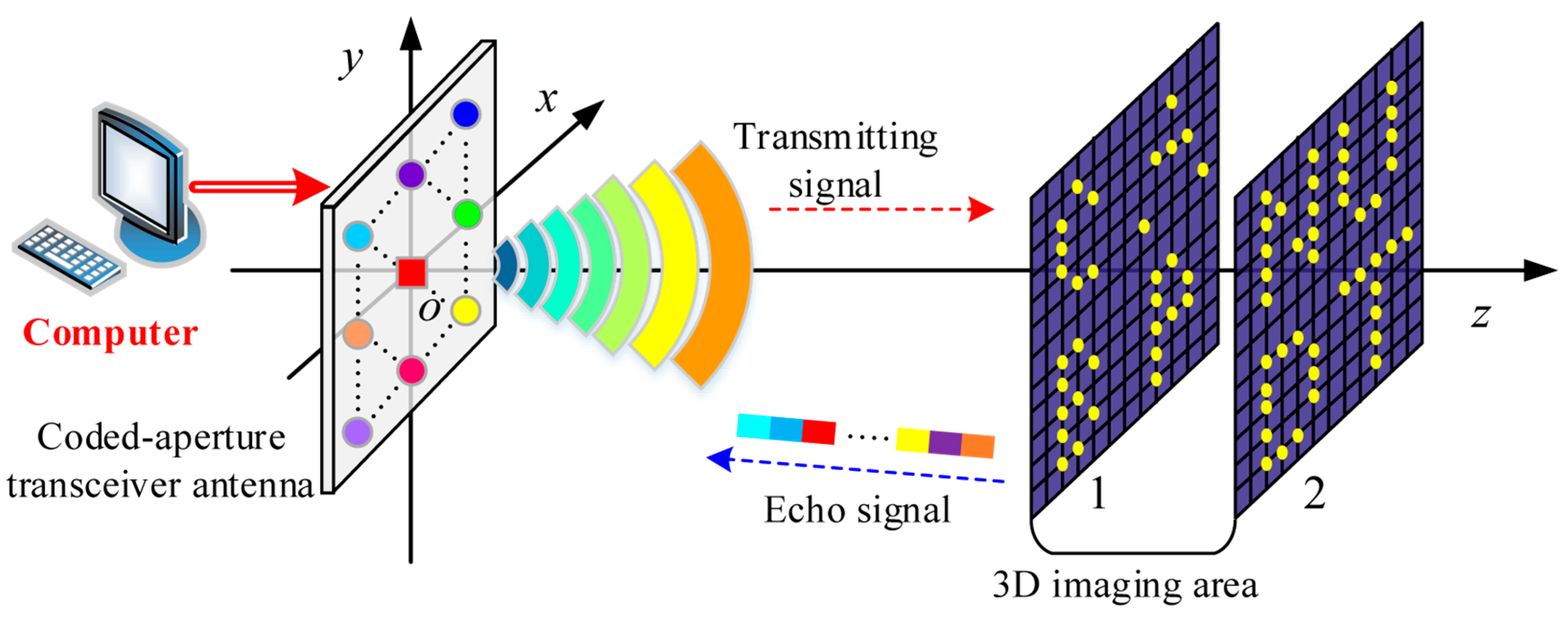
| Requirement | A Computer and a Coded-Aperture Array Transceiver. |
|---|---|
| Imaging process | Step 1: Obtain the time domain echo signal by the following procedures. (1) The computer controls the single transmitter to send signals. (2) Multiple coded-aperture detectors randomly modulate and receive the echo signals. (3) The modulated echo signals are transported into the computer for imaging. |
| Step 2: parfor x = 1:X parfor a = 1:A (A describes the imaging-area numbers in imaging plane x)
end | |
| Step 3: Obtain the 3D imaging result in combination of . | |
| Output | Return the BP-TCAI imaging result . |
| Parameter | Value |
|---|---|
| Center frequency (fc) | 340 GHz |
| Bandwidth (B) | 20 GHz |
| Pulse Width (Tp) | 100 ns |
| Size of the coded aperture | 0.5 m × 0.5 m |
| Number of coded-aperture array elements | 25 × 25 |
| Range of Scene 1 | 1.5 m |
| Range of Scene 2 | 2 m |
| Range of Scene 3 | 2.5 m |
| Range of Scene 4 | 3 m |
| Size of the grid cell | 0.0025 m × 0.0025 m |
| BP-TCAI | GM-TCAI | TCAI |
|---|---|---|
| 2.4258 | 8.7253 | 16.8327 |
© 2018 by the authors. Licensee MDPI, Basel, Switzerland. This article is an open access article distributed under the terms and conditions of the Creative Commons Attribution (CC BY) license (http://creativecommons.org/licenses/by/4.0/).
Share and Cite
Chen, S.; Luo, C.; Wang, H.; Wang, W.; Peng, L.; Zhuang, Z. Three-Dimensional Terahertz Coded-Aperture Imaging Based on Back Projection. Sensors 2018, 18, 2510. https://doi.org/10.3390/s18082510
Chen S, Luo C, Wang H, Wang W, Peng L, Zhuang Z. Three-Dimensional Terahertz Coded-Aperture Imaging Based on Back Projection. Sensors. 2018; 18(8):2510. https://doi.org/10.3390/s18082510
Chicago/Turabian StyleChen, Shuo, Chenggao Luo, Hongqiang Wang, Wenpeng Wang, Long Peng, and Zhaowen Zhuang. 2018. "Three-Dimensional Terahertz Coded-Aperture Imaging Based on Back Projection" Sensors 18, no. 8: 2510. https://doi.org/10.3390/s18082510
APA StyleChen, S., Luo, C., Wang, H., Wang, W., Peng, L., & Zhuang, Z. (2018). Three-Dimensional Terahertz Coded-Aperture Imaging Based on Back Projection. Sensors, 18(8), 2510. https://doi.org/10.3390/s18082510