Figure 1.
High level system block diagram for the proposed ultra-wideband imaging system.
Figure 1.
High level system block diagram for the proposed ultra-wideband imaging system.
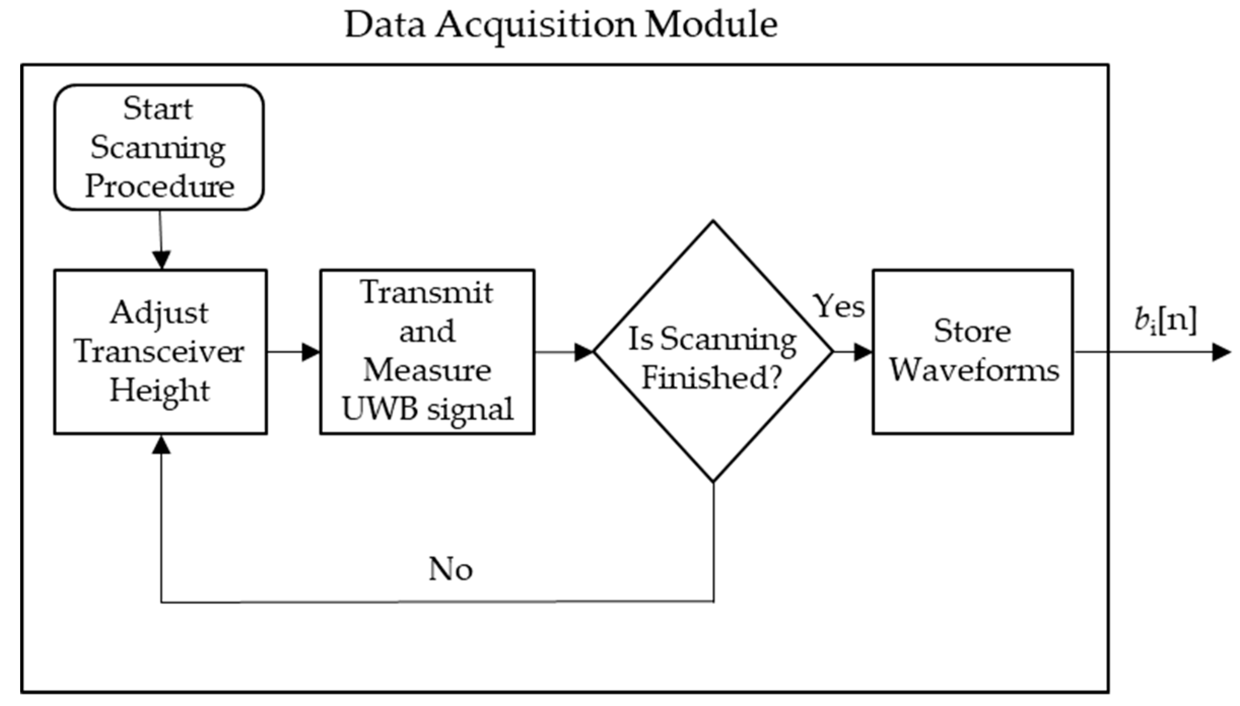
Figure 2.
Process for the scanning procedure process for both simulated and experimental trials.
Figure 2.
Process for the scanning procedure process for both simulated and experimental trials.
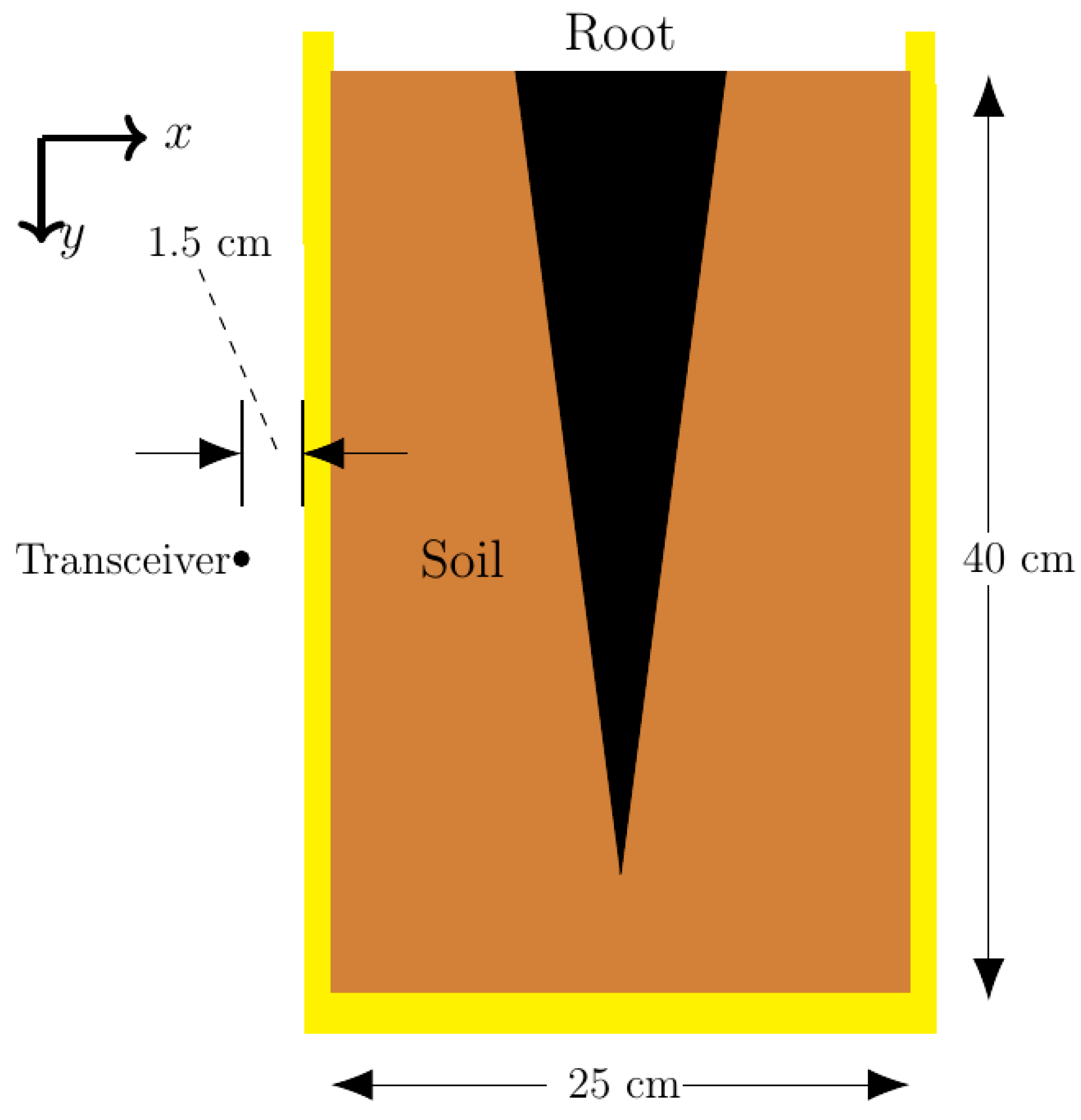
Figure 3.
Physical parameters on pot and root model.
Figure 3.
Physical parameters on pot and root model.
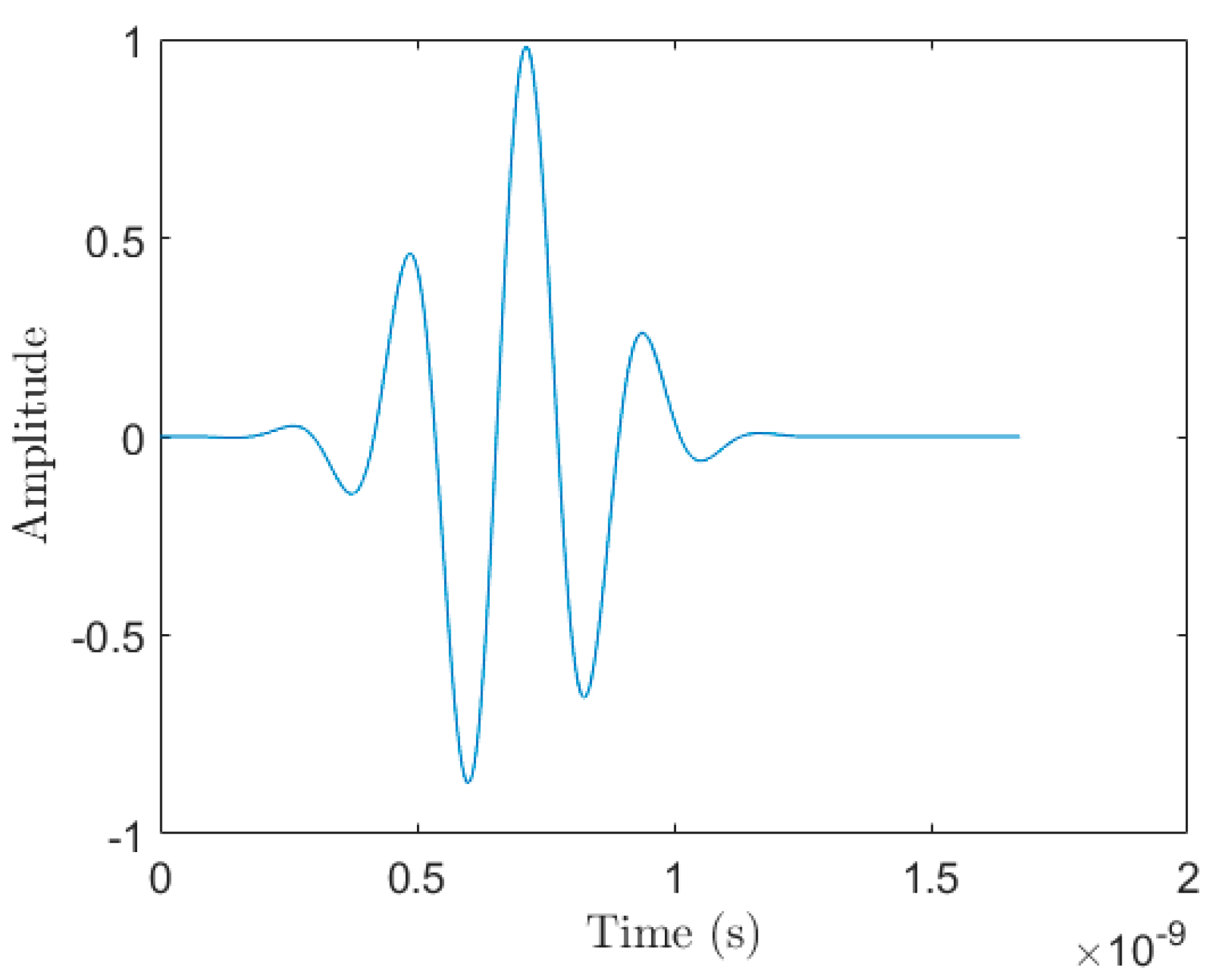
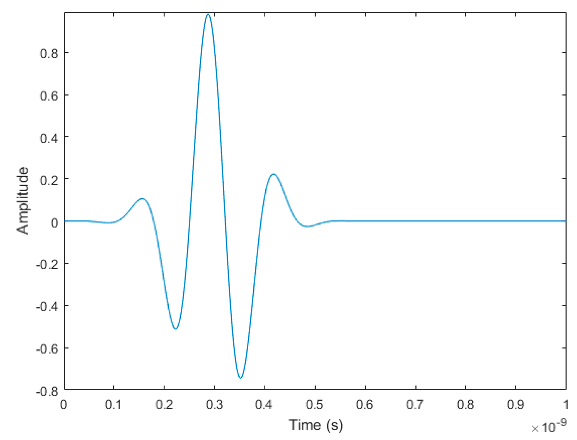
Figure 4.
The 3.1 GHz to 5.3 GHz source waveform, , used in the 2D simulations.
Figure 4.
The 3.1 GHz to 5.3 GHz source waveform, , used in the 2D simulations.
Figure 5.
Apparatus set-up for scanning buried roots.
Figure 5.
Apparatus set-up for scanning buried roots.
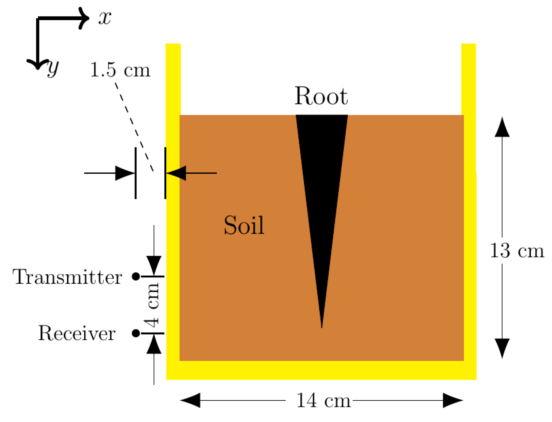
Figure 6.
Experimental apparatus set-up dimensions for scanning buried roots.
Figure 6.
Experimental apparatus set-up dimensions for scanning buried roots.
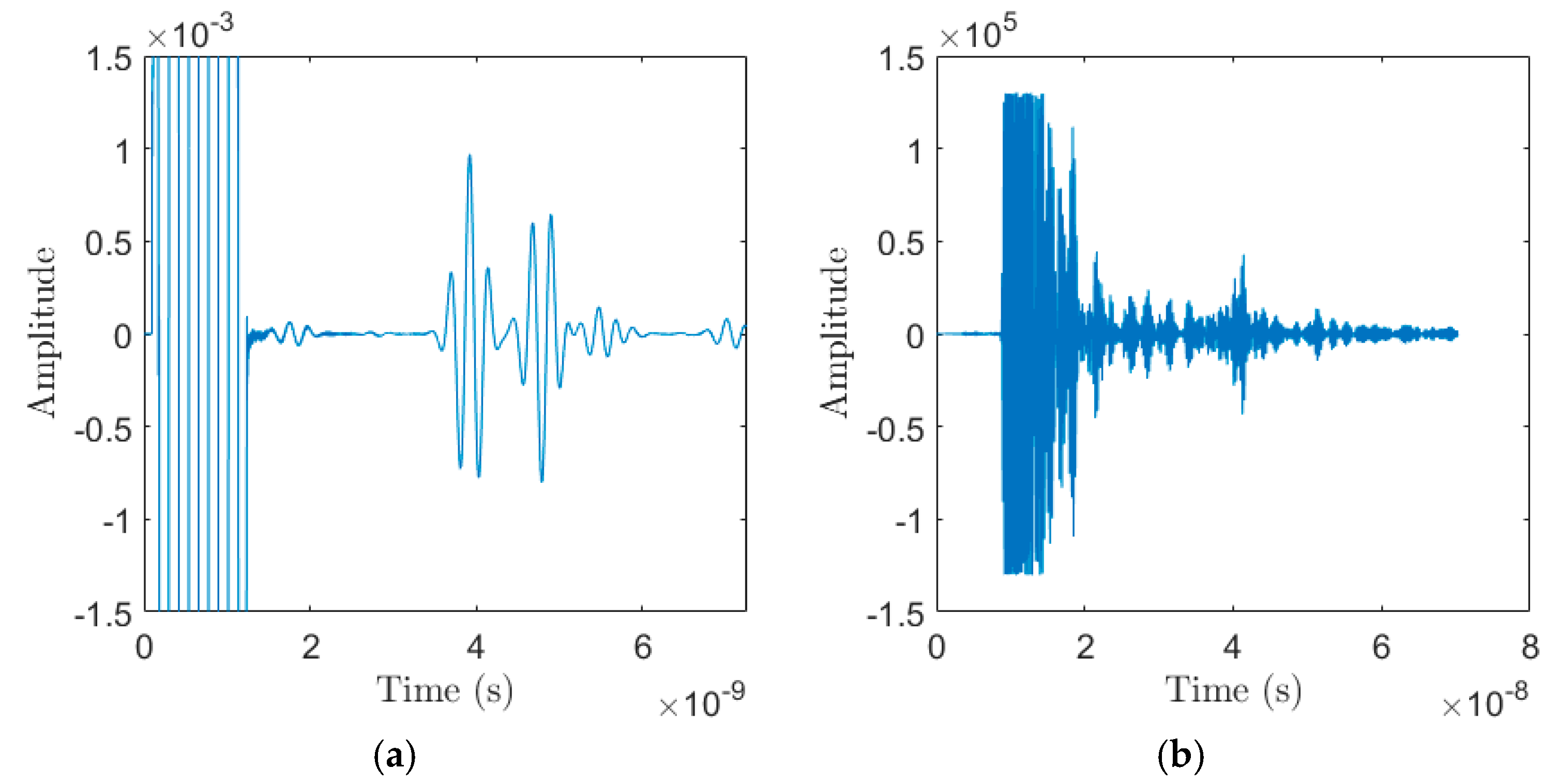
Figure 7.
Data Acquisition Module output: (a) Example of a measured reflected waveform in simulated trials; (b) Example of a measured reflected waveform in experimental trials.
Figure 7.
Data Acquisition Module output: (a) Example of a measured reflected waveform in simulated trials; (b) Example of a measured reflected waveform in experimental trials.
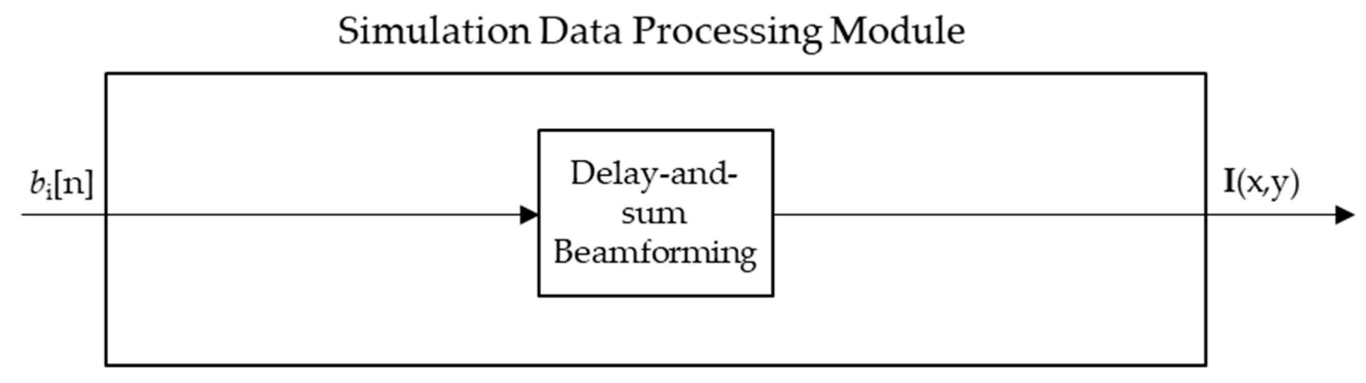
Figure 8.
Data Processing Module blocks for the simulated trials.
Figure 8.
Data Processing Module blocks for the simulated trials.
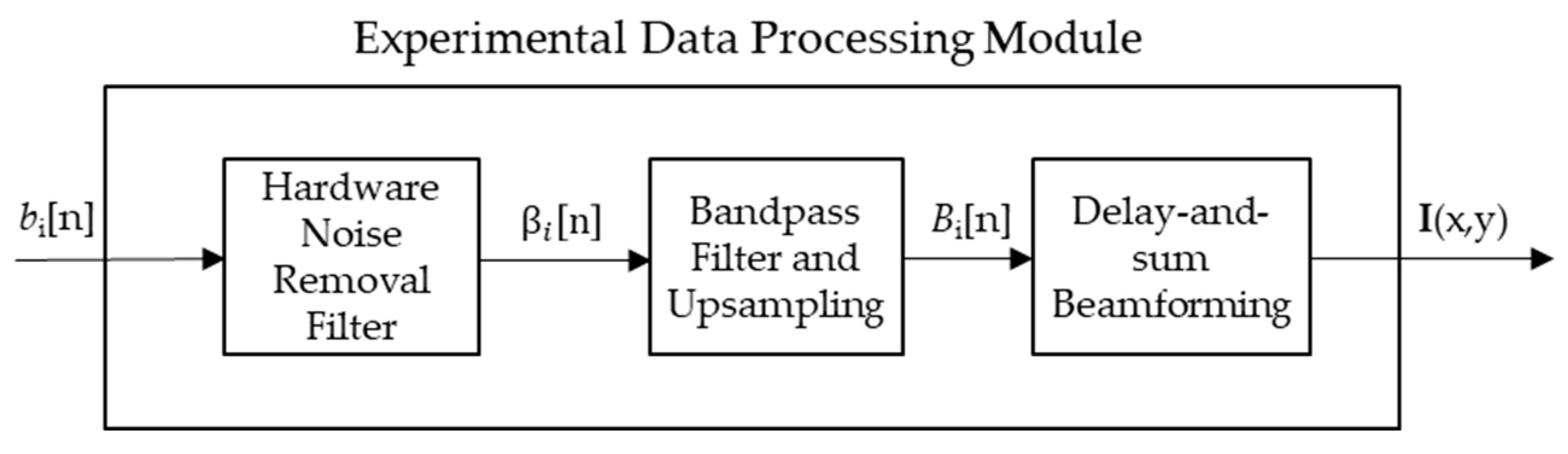
Figure 9.
Data Processing Module blocks for the experimental trials.
Figure 9.
Data Processing Module blocks for the experimental trials.
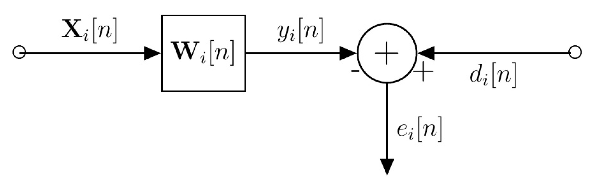
Figure 10.
Block diagram for hardware noise removal system.
Figure 10.
Block diagram for hardware noise removal system.
Figure 11.
The measured reflected signal with the hardware noise removed, .
Figure 11.
The measured reflected signal with the hardware noise removed, .
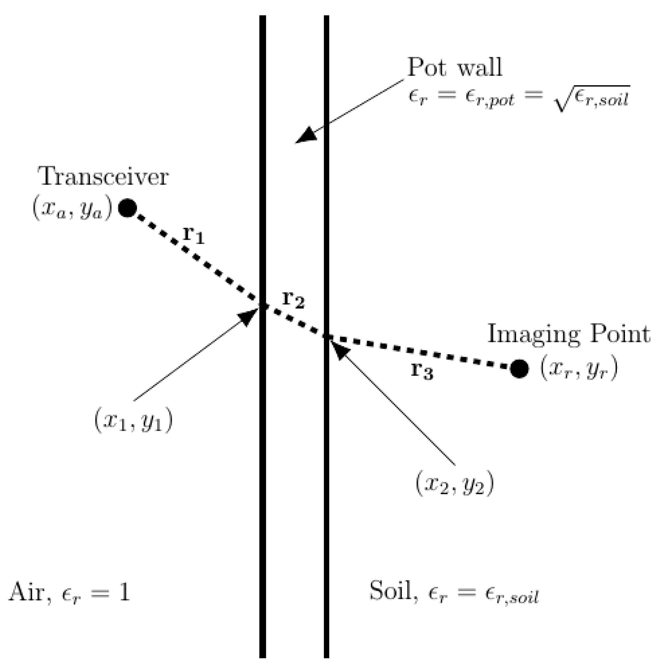
Figure 12.
Most direct path from transceiver to imaging point for use in delay-and-sum (DAS) beamforming.
Figure 12.
Most direct path from transceiver to imaging point for use in delay-and-sum (DAS) beamforming.
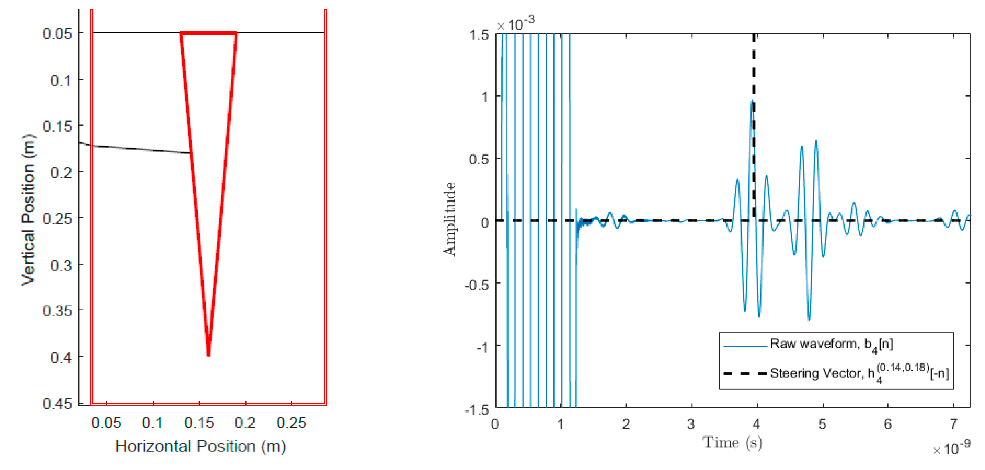
Figure 13.
Scan position 4 and calculated ray path for the emitted ultra-wideband (UWB) pulse to point (0.14, 0.18).
Figure 13.
Scan position 4 and calculated ray path for the emitted ultra-wideband (UWB) pulse to point (0.14, 0.18).
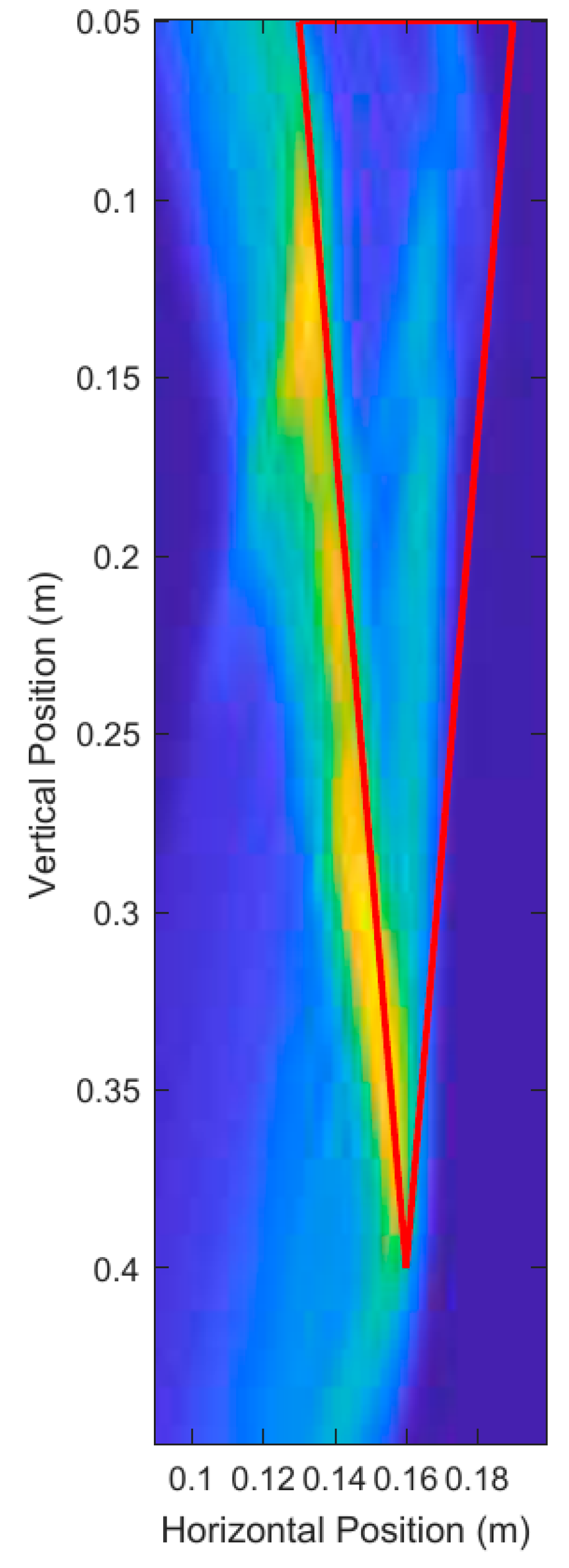
Figure 14.
Scan position 4 and calculated ray path for emitted UWB pulse to point (0.14, 0.18). The thick red lines indicate the true position of the root and are not a part of the output of the system.
Figure 14.
Scan position 4 and calculated ray path for emitted UWB pulse to point (0.14, 0.18). The thick red lines indicate the true position of the root and are not a part of the output of the system.
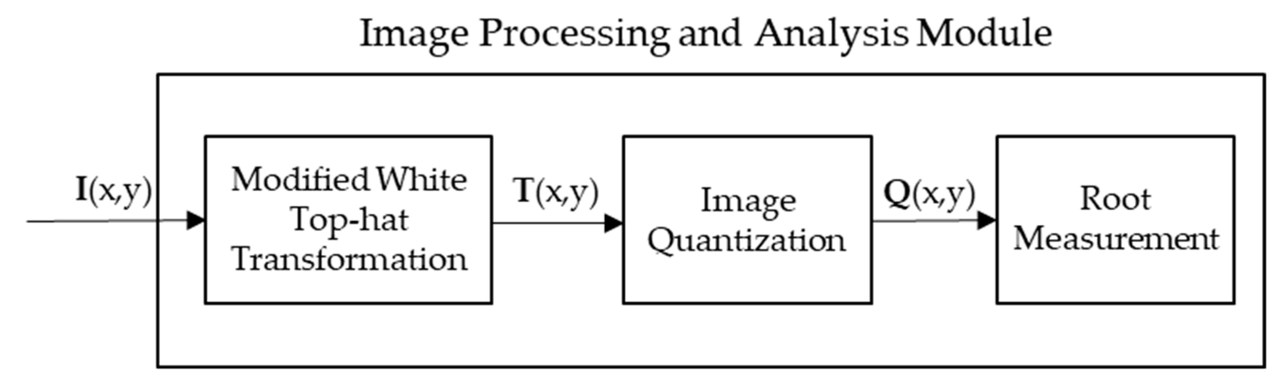
Figure 15.
Image Processing and Analysis Module blocks for simulated and experimental trials.
Figure 15.
Image Processing and Analysis Module blocks for simulated and experimental trials.
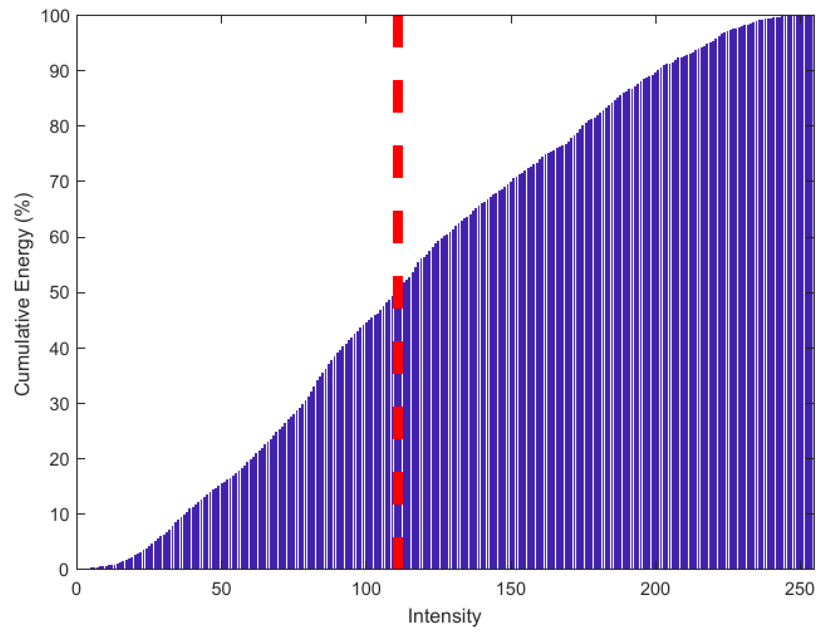
Figure 16.
Cumulative energy histogram for
shown in
Figure 14. The red dashed line indicates the 50% energy threshold.
Figure 16.
Cumulative energy histogram for
shown in
Figure 14. The red dashed line indicates the 50% energy threshold.
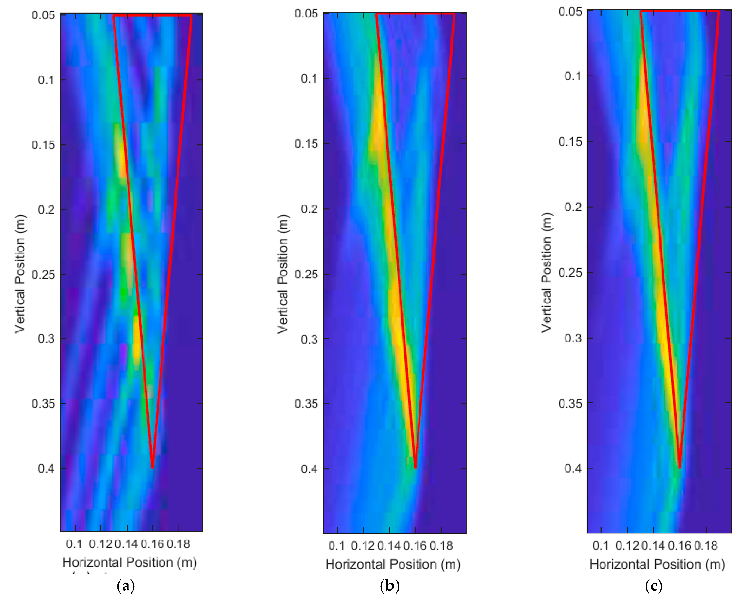
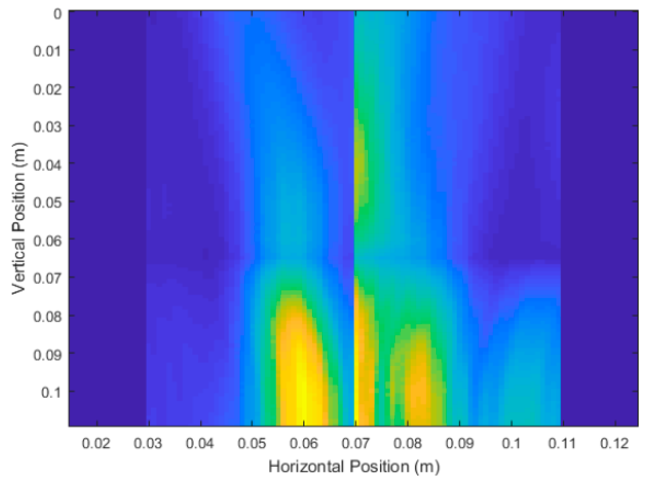
Figure 17.
Unprocessed DAS beamforming images for: (a) six scanning positions, (b) 12 scanning positions, and (c) 21 scanning positions.
Figure 17.
Unprocessed DAS beamforming images for: (a) six scanning positions, (b) 12 scanning positions, and (c) 21 scanning positions.
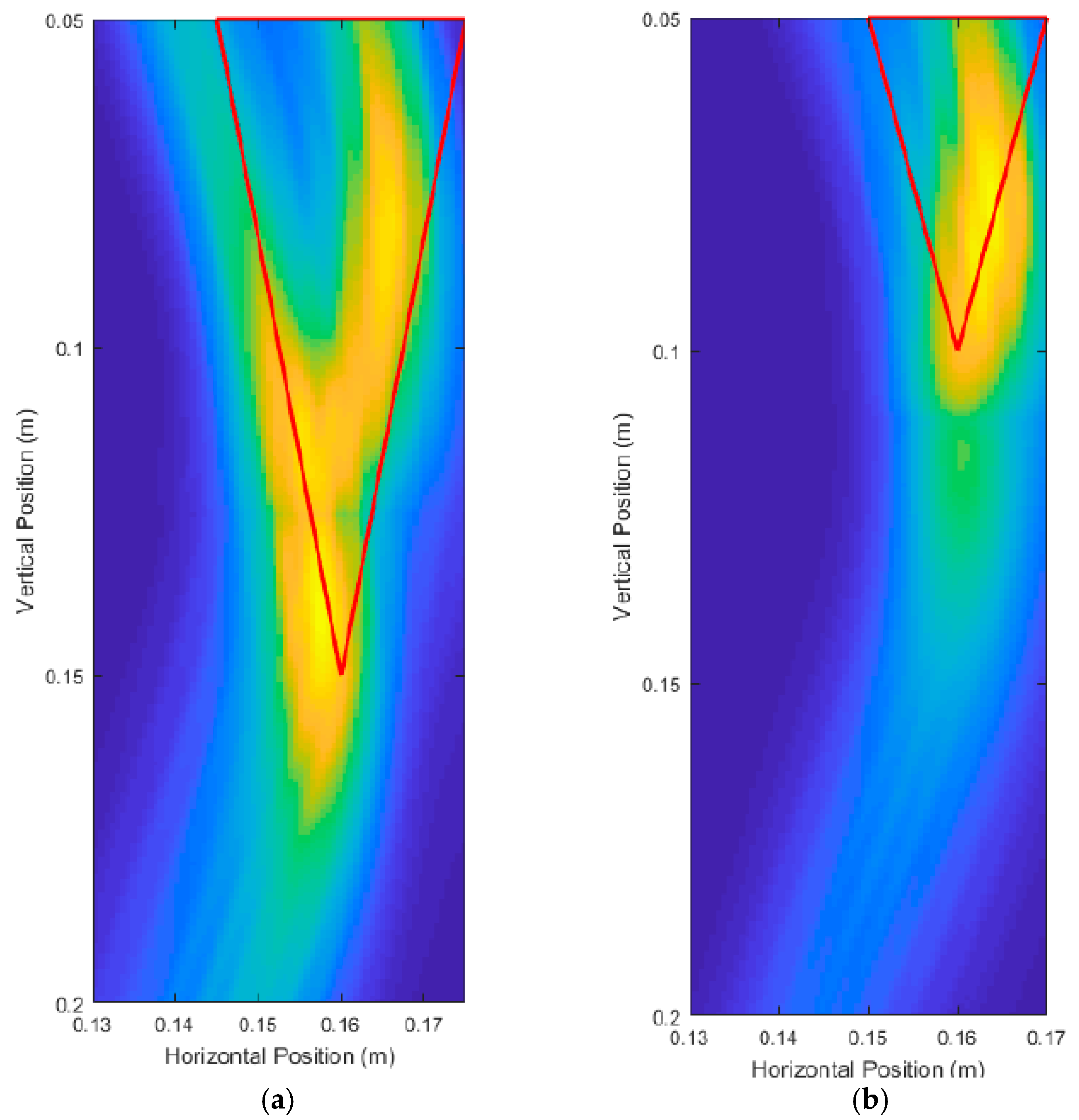
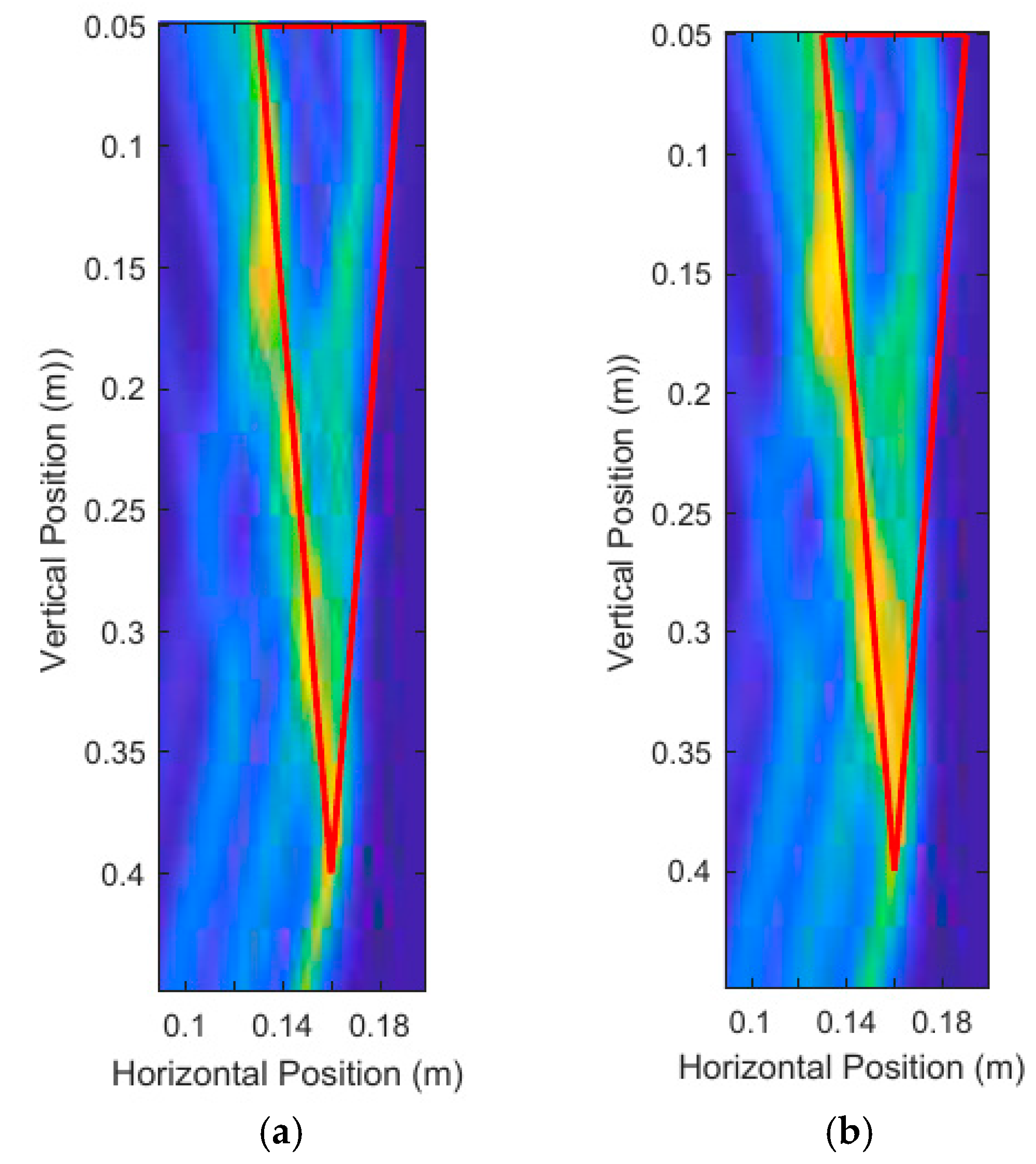
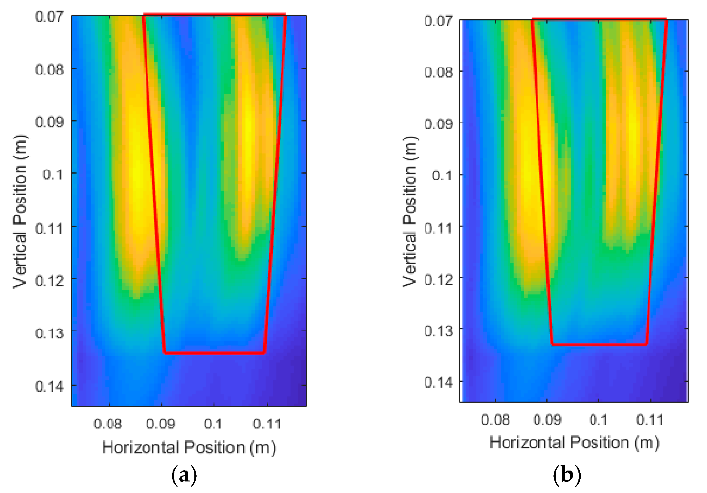
Figure 18.
Unprocessed DAS beamforming images for a root with: (a) 10.00 cm depth and 1.50 cm average diameter, and (b) 5.00 cm depth and 1.00 cm average diameter.
Figure 18.
Unprocessed DAS beamforming images for a root with: (a) 10.00 cm depth and 1.50 cm average diameter, and (b) 5.00 cm depth and 1.00 cm average diameter.
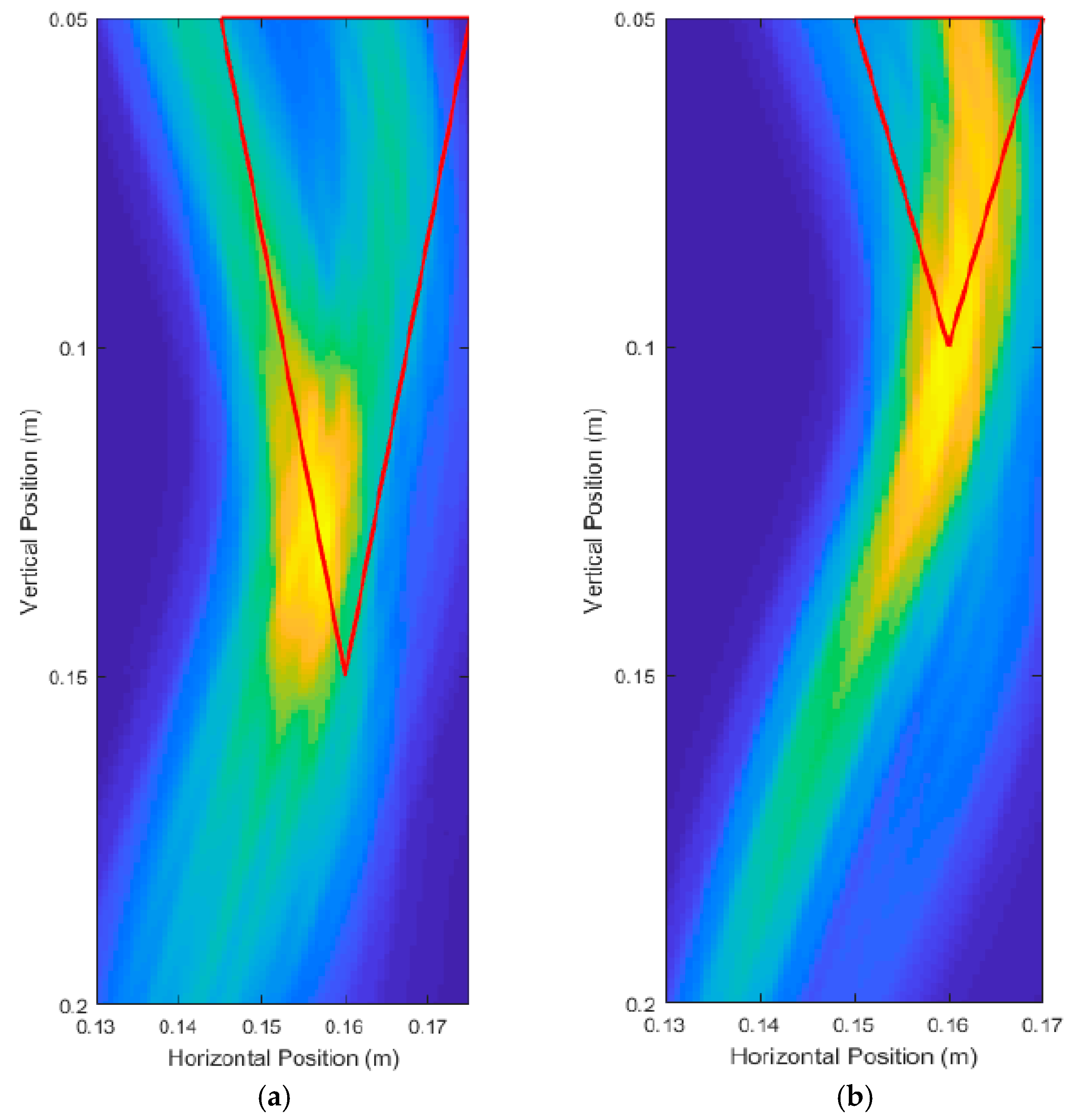
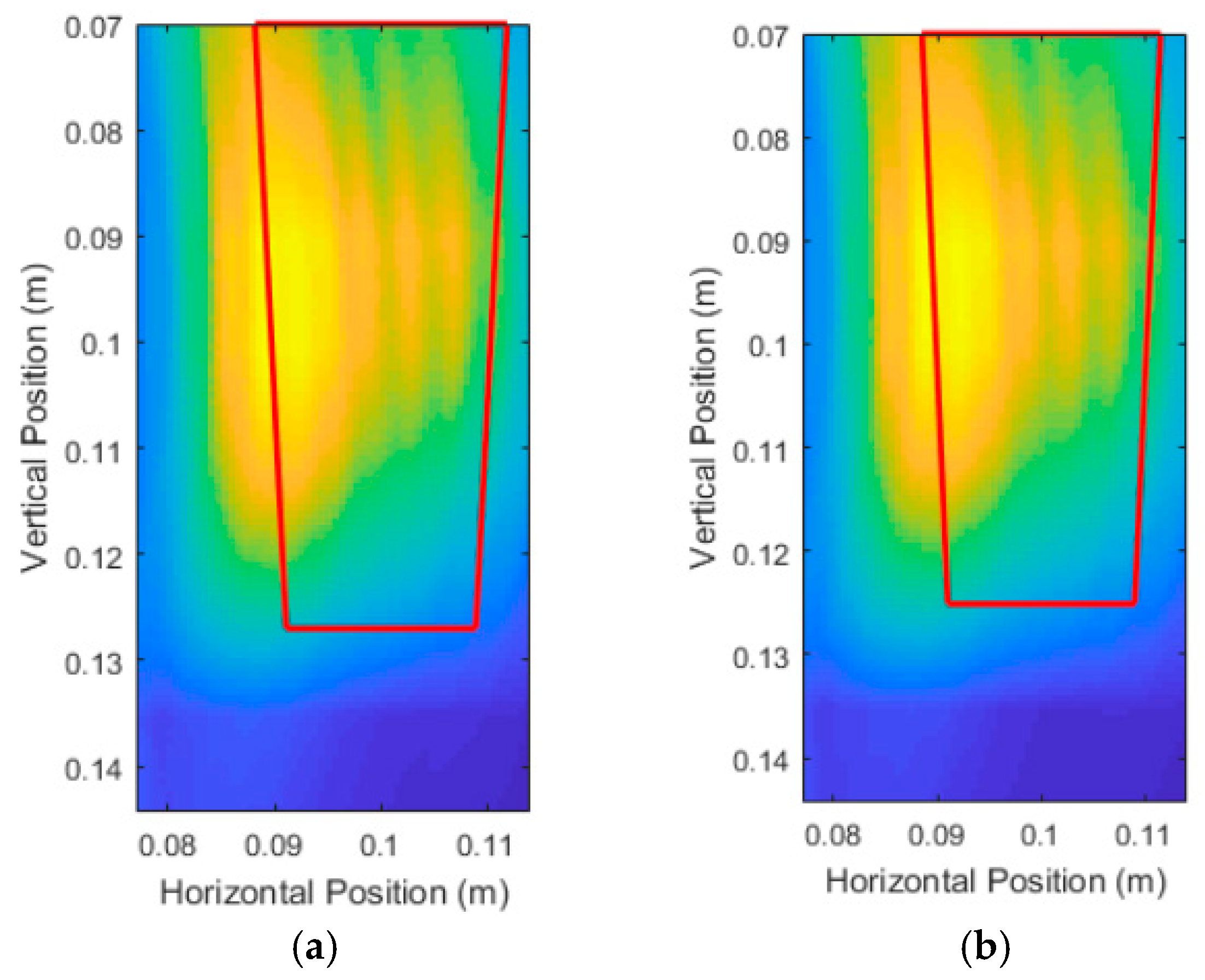
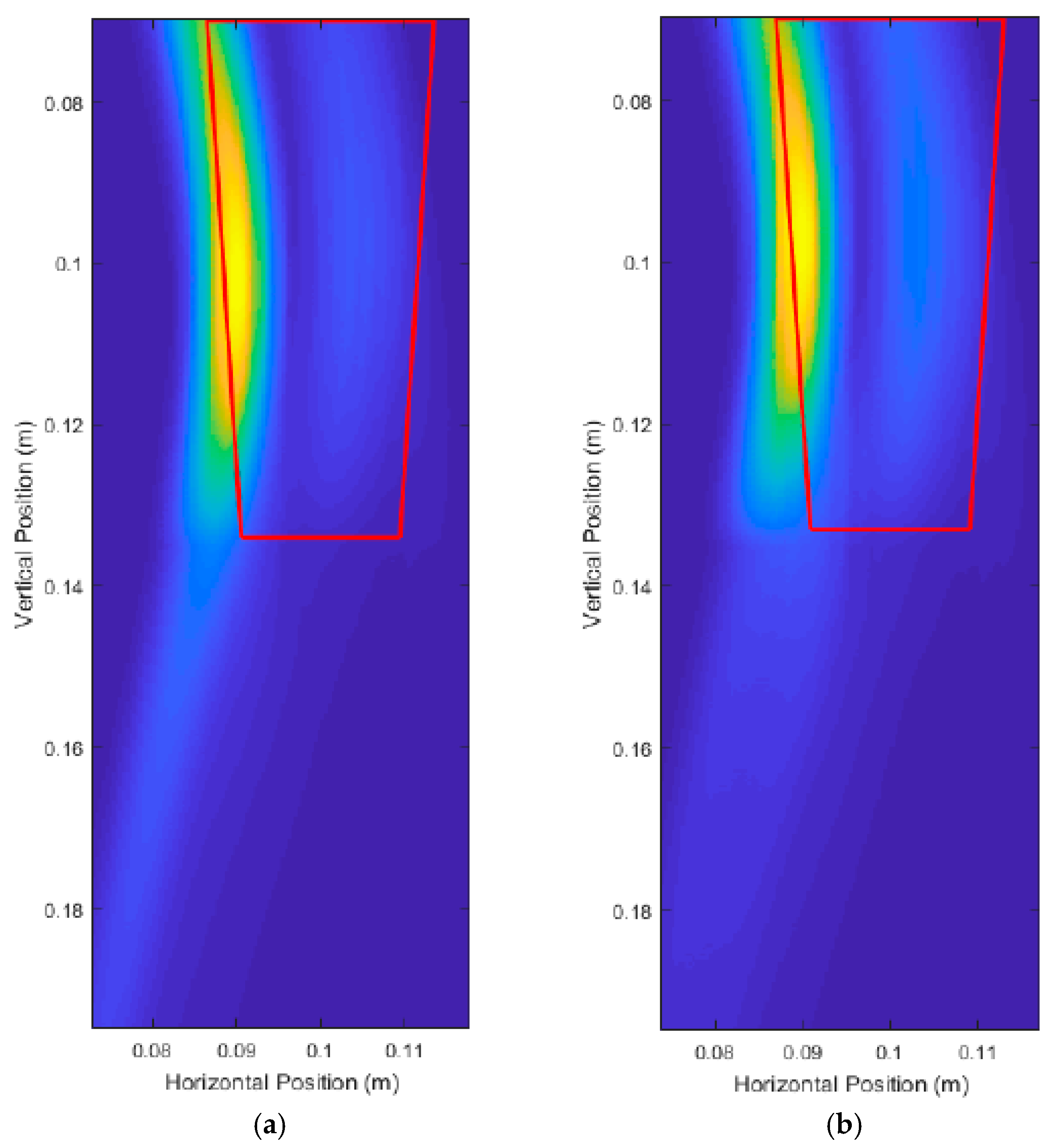
Figure 19.
Unprocessed DAS beamforming images with a shortened scan range (decreased scan spacing) for a root with: (a) 10.00 cm depth and 1.50 cm average diameter, and (b) 5.00 cm depth and 1.00 cm average diameter.
Figure 19.
Unprocessed DAS beamforming images with a shortened scan range (decreased scan spacing) for a root with: (a) 10.00 cm depth and 1.50 cm average diameter, and (b) 5.00 cm depth and 1.00 cm average diameter.
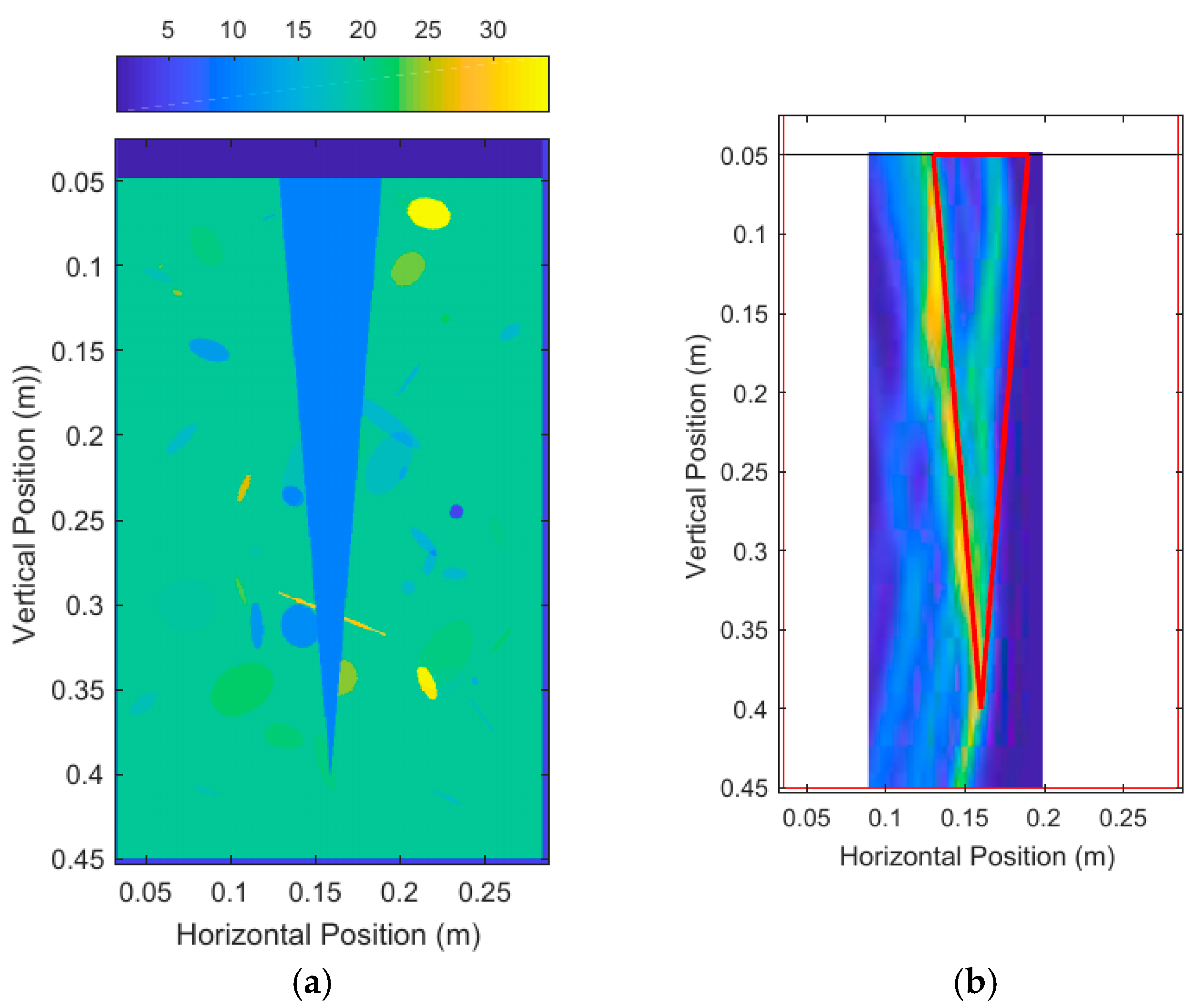
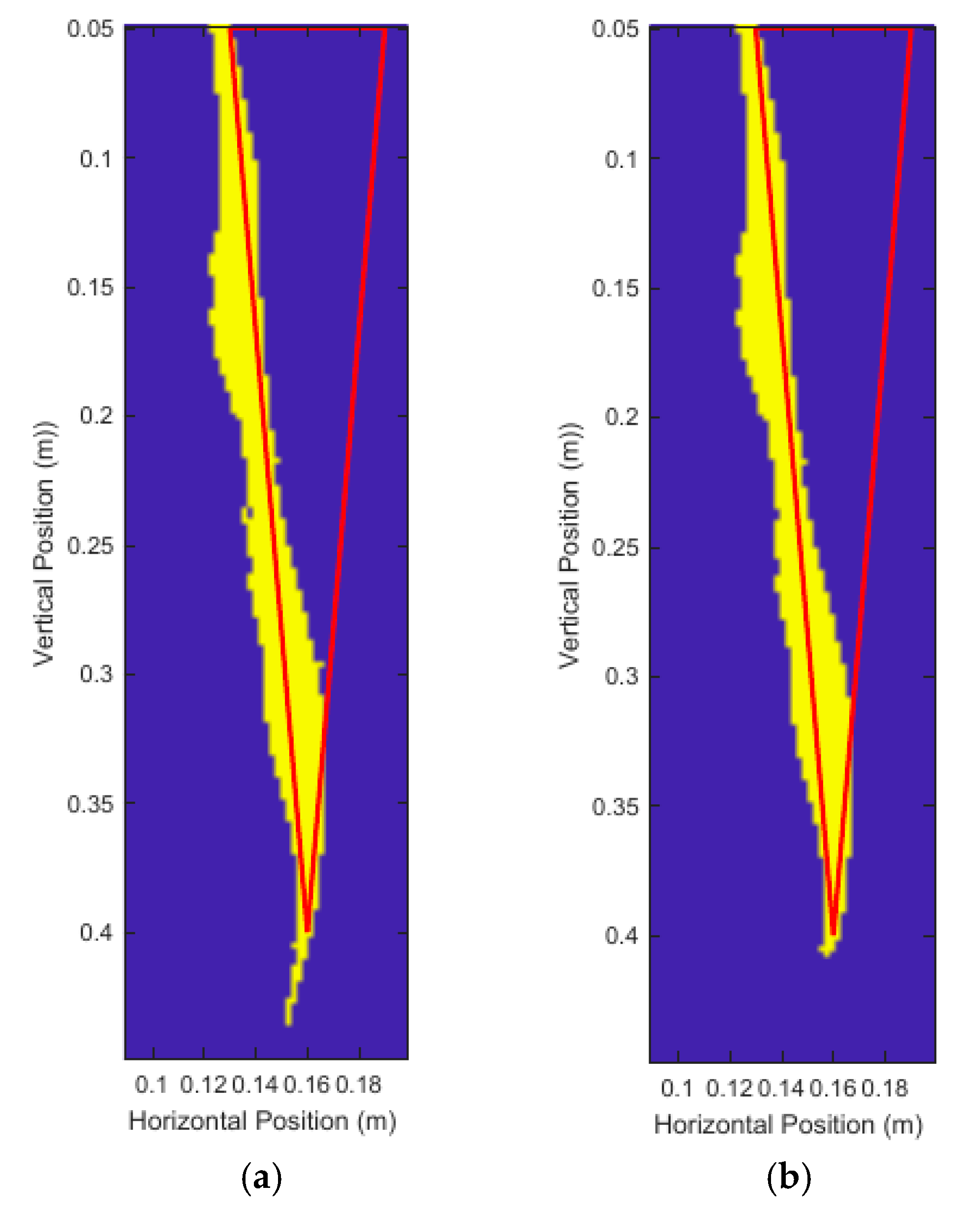
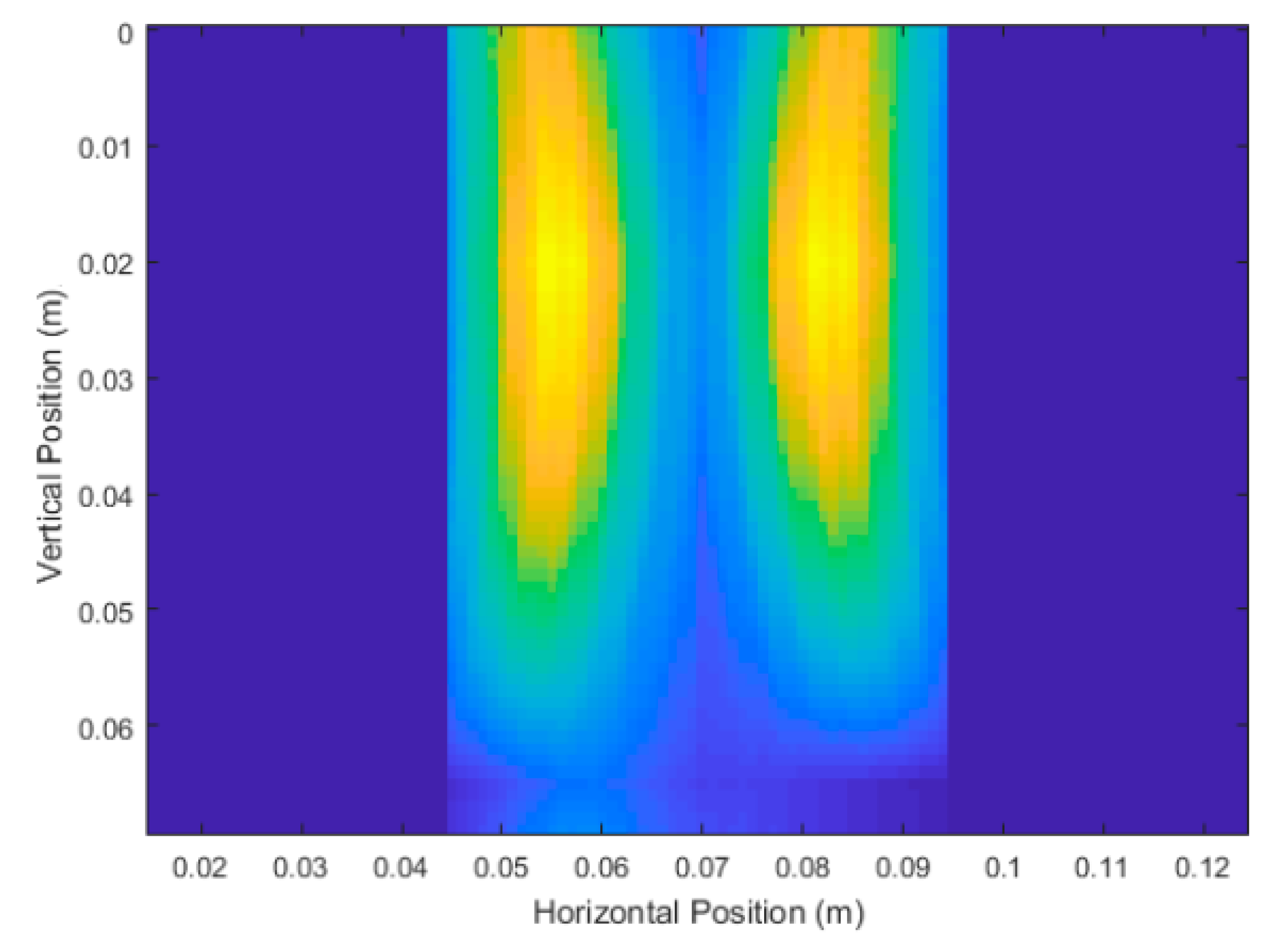
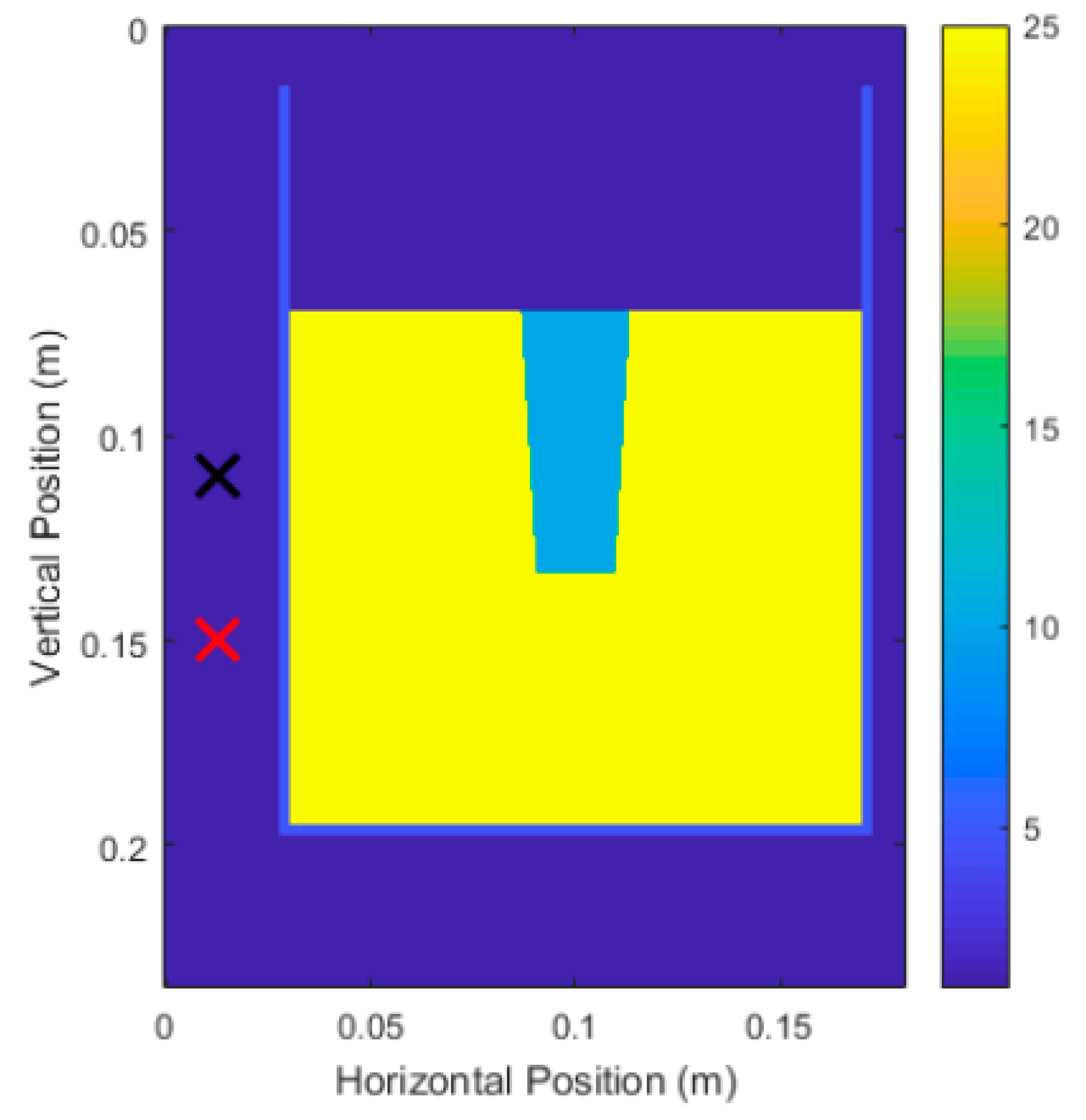
Figure 20.
The noisy system under test containing a root with where: (a) is the relative permittivity distribution of the simulated system and (b) is the unprocessed DAS beamforming image for the simulated system.
Figure 20.
The noisy system under test containing a root with where: (a) is the relative permittivity distribution of the simulated system and (b) is the unprocessed DAS beamforming image for the simulated system.
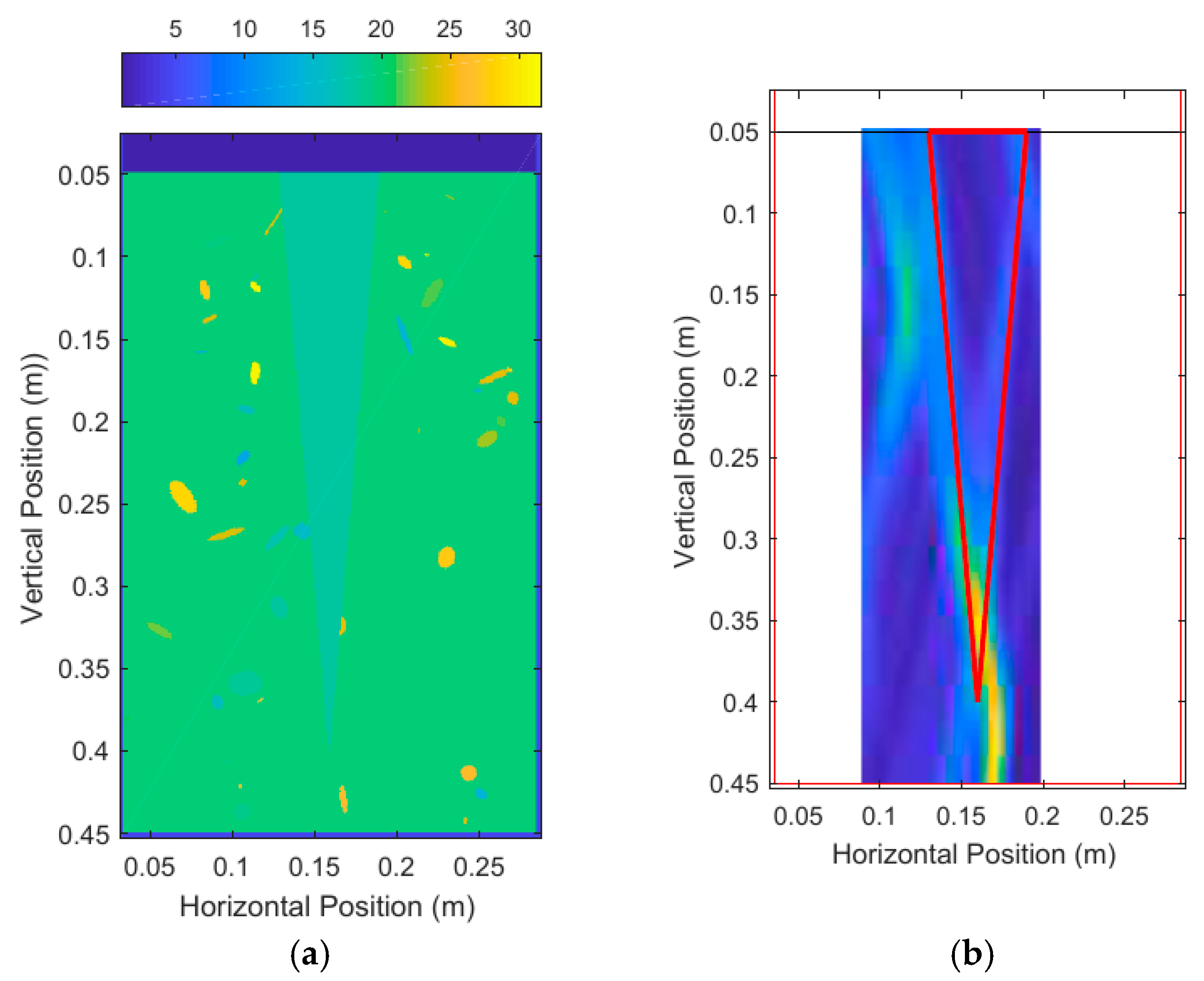
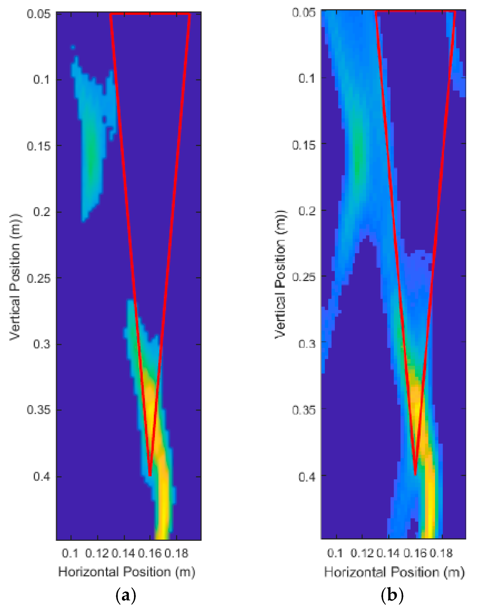
Figure 21.
The noisy system under test containing a root with where: (a) is the relative permittivity distribution of the simulated system and (b) is the unprocessed DAS beamforming image for the simulated system.
Figure 21.
The noisy system under test containing a root with where: (a) is the relative permittivity distribution of the simulated system and (b) is the unprocessed DAS beamforming image for the simulated system.
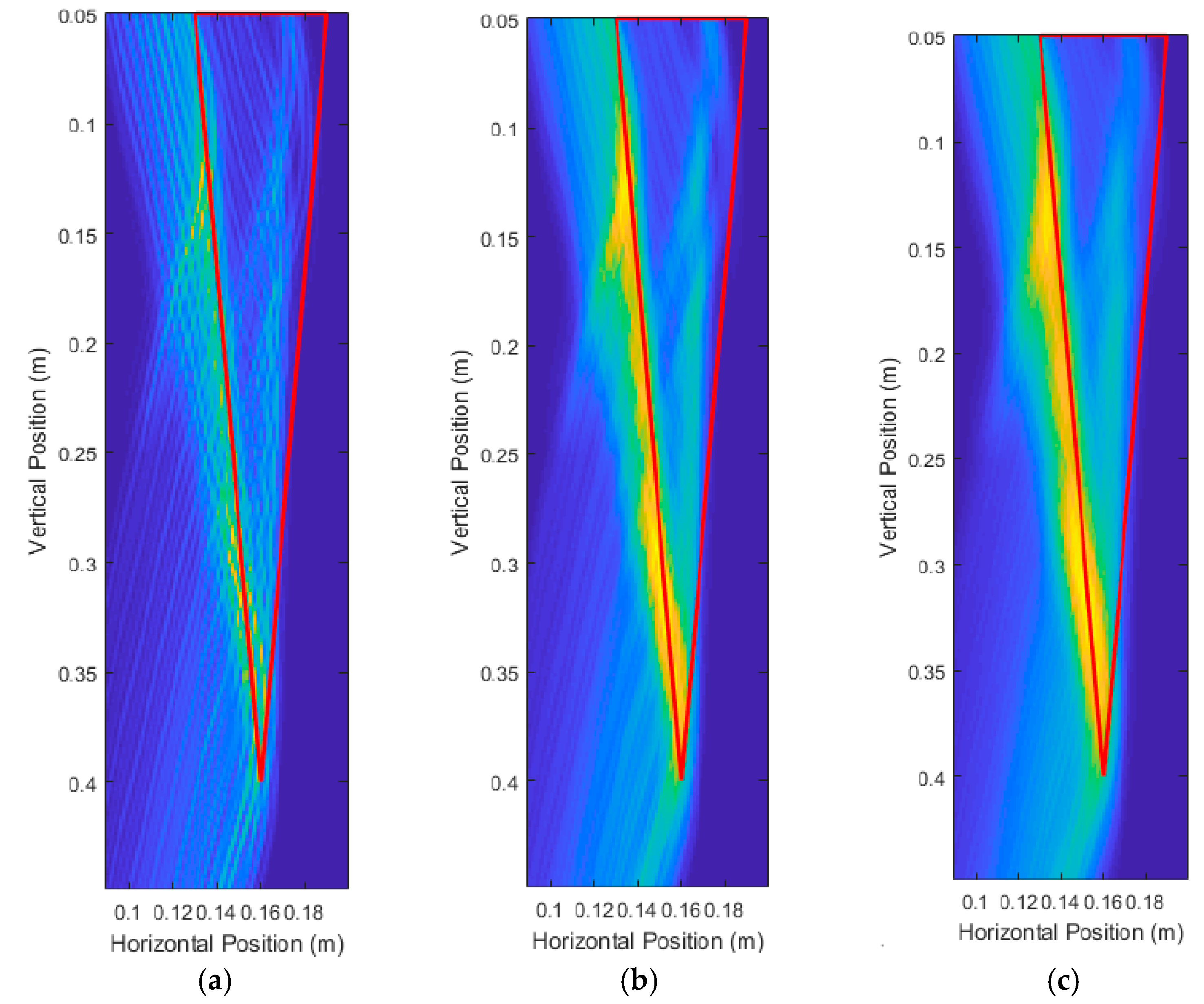
Figure 22.
Unprocessed DAS beamforming images where is set to be: (a) quarter carrier cycle length, (b) half carrier cycle length, and (c) one-and-half carrier cycle length.
Figure 22.
Unprocessed DAS beamforming images where is set to be: (a) quarter carrier cycle length, (b) half carrier cycle length, and (c) one-and-half carrier cycle length.
Figure 23.
DAS beamforming results for: (a) the unprocessed image and (b) the image after the modified top-hat transformation.
Figure 23.
DAS beamforming results for: (a) the unprocessed image and (b) the image after the modified top-hat transformation.
Figure 24.
Binary masks for: (a) no binary erosion performed and (b) a binary erosion and dilation performed.
Figure 24.
Binary masks for: (a) no binary erosion performed and (b) a binary erosion and dilation performed.
Figure 25.
Comparison of a high noise images with: (a) 35% percent energy retained and (b) 70% percent energy retained.
Figure 25.
Comparison of a high noise images with: (a) 35% percent energy retained and (b) 70% percent energy retained.
Figure 26.
Unprocessed DAS beamforming results of Carrot 1 Side 1 with vertical scans taken at 0° and 180°, depth measurements after processing of 5.7 cm and 5.8 cm respectively. Average diameter after processing measured to be 2.85 cm.
Figure 26.
Unprocessed DAS beamforming results of Carrot 1 Side 1 with vertical scans taken at 0° and 180°, depth measurements after processing of 5.7 cm and 5.8 cm respectively. Average diameter after processing measured to be 2.85 cm.
Figure 27.
Unprocessed DAS beamforming results of Carrot 1 Side 2 with vertical scans taken at 90° and 270°, depth measurements after processing of 5.7 cm and 6.4 cm respectively. Average diameter after processing measured to be 2.36 cm.
Figure 27.
Unprocessed DAS beamforming results of Carrot 1 Side 2 with vertical scans taken at 90° and 270°, depth measurements after processing of 5.7 cm and 6.4 cm respectively. Average diameter after processing measured to be 2.36 cm.
Figure 28.
Unprocessed DAS beamforming results of Carrot 2 Side 1, with vertical scans taken at 0° and 180°, and depth measurements after processing of 5.5 cm and 5.1 cm respectively. Average diameter after processing was measured to be 2.40 cm.
Figure 28.
Unprocessed DAS beamforming results of Carrot 2 Side 1, with vertical scans taken at 0° and 180°, and depth measurements after processing of 5.5 cm and 5.1 cm respectively. Average diameter after processing was measured to be 2.40 cm.
Figure 29.
Unprocessed DAS beamforming results of Carrot 2 Side 2, with vertical scans taken at 90° and 270°, and depth measurements after processing of 5.6 cm and 5.3 cm respectively. Average diameter after processing was measured to be 2.63 cm.
Figure 29.
Unprocessed DAS beamforming results of Carrot 2 Side 2, with vertical scans taken at 90° and 270°, and depth measurements after processing of 5.6 cm and 5.3 cm respectively. Average diameter after processing was measured to be 2.63 cm.
Figure 30.
Physical and electrical parameters of system under test which models the experimental trials.
Figure 30.
Physical and electrical parameters of system under test which models the experimental trials.
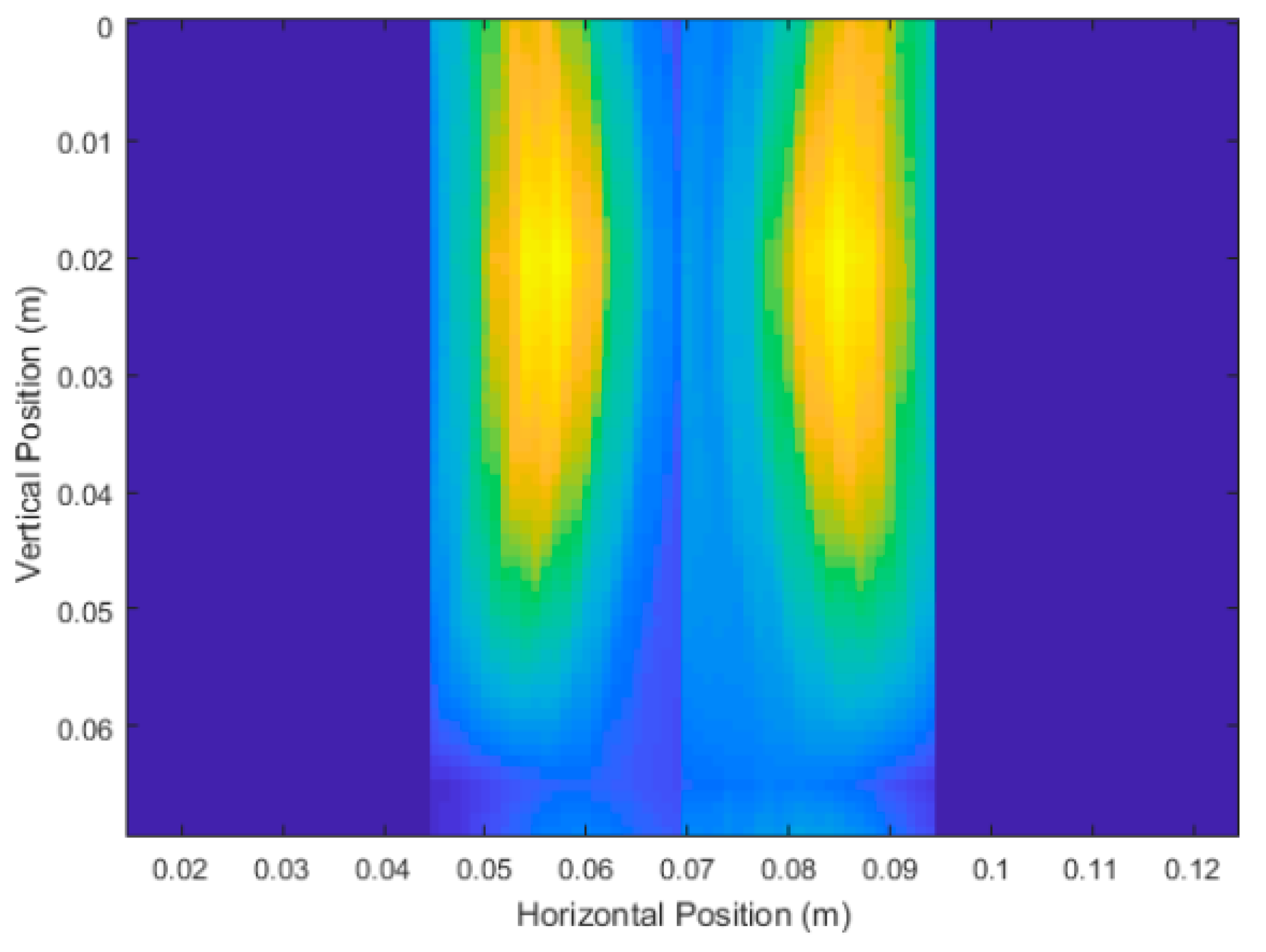
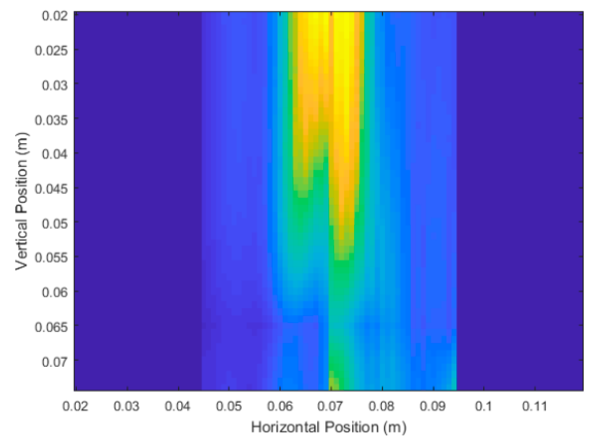
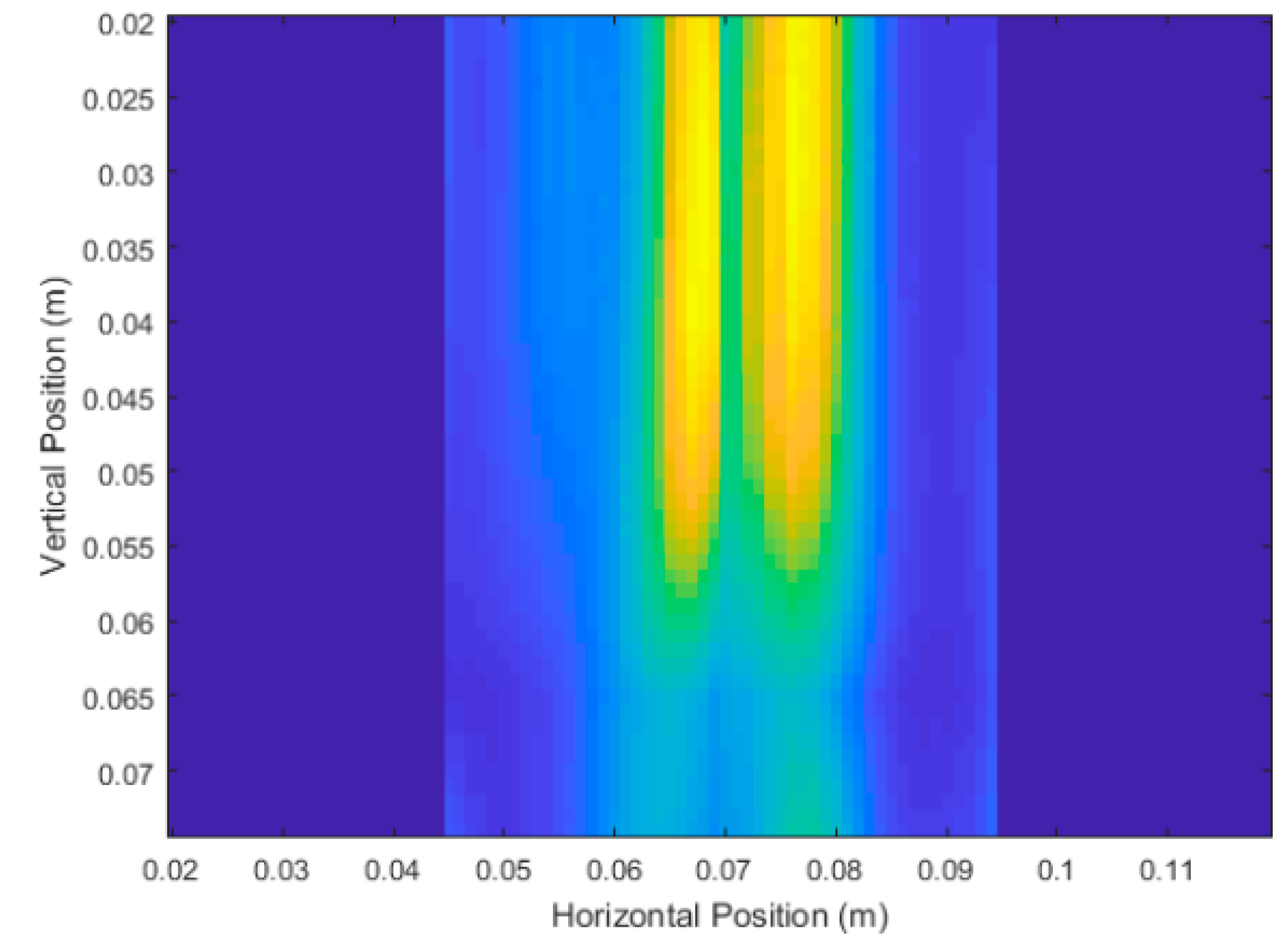
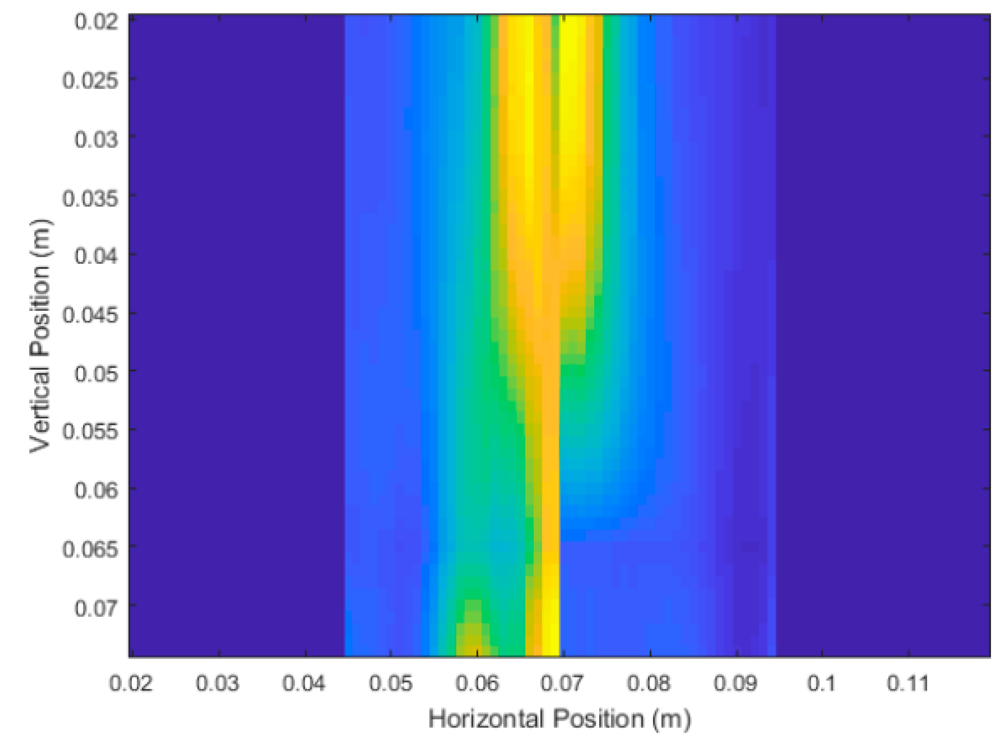
Figure 31.
Unprocessed DAS beamforming images of the experimental replication trials for: (a) Carrot 1, Side 1 and (b) Carrot 1, Side 2.
Figure 31.
Unprocessed DAS beamforming images of the experimental replication trials for: (a) Carrot 1, Side 1 and (b) Carrot 1, Side 2.
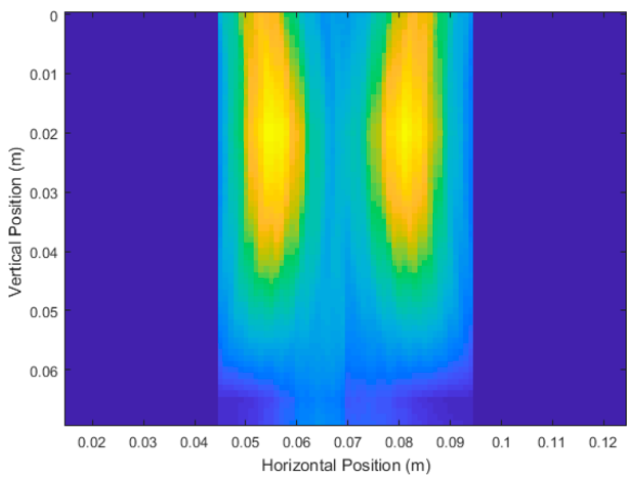
Figure 32.
Unprocessed DAS beamforming images of the experimental replication trials for: (a) Carrot 2, Side 1 and (b) Carrot 2, Side 2.
Figure 32.
Unprocessed DAS beamforming images of the experimental replication trials for: (a) Carrot 2, Side 1 and (b) Carrot 2, Side 2.
Figure 33.
2 GHz to 12 GHz waveform used in high frequency simulations.
Figure 33.
2 GHz to 12 GHz waveform used in high frequency simulations.
Figure 34.
Unprocessed DAS beamforming images using a high frequency source pulse for: (a) Carrot 1, Side 1 and (b) Carrot 1, Side 2.
Figure 34.
Unprocessed DAS beamforming images using a high frequency source pulse for: (a) Carrot 1, Side 1 and (b) Carrot 1, Side 2.
Table 1.
Measured root depths and average root diameters for images produced by varying the number of scanning positions.
Table 1.
Measured root depths and average root diameters for images produced by varying the number of scanning positions.
| Number of Scans | Measured Root Depth (cm) | Error in Depth Measurement (cm) | Measured Average Root Diameter (cm) | Error in Average Diameter Measurement (cm) |
|---|
| 6 | 30.25 | −5.75 | 3.85 | +0.85 |
| 12 | 36.14 | +1.14 | 3.14 | +0.14 |
| 21 | 34.69 | −0.31 | 3.29 | +0.29 |
Table 2.
Measured root depths and root average diameters for images produced by varying the number of scanning positions.
Table 2.
Measured root depths and root average diameters for images produced by varying the number of scanning positions.
| Root Depth (cm) | Percent Error in Depth Measurement (%) | Average Root Diameter (cm) | Percent Error in Average Root Diameter Measurement (%) |
|---|
| 25.00 | 4.3 | 2.00 | 15.6 |
| 15.00 | 13.5 | 1.50 | 26.4 |
| 10.00 | 30.4 | 1.50 | 18.7 |
| 5.00 | 112.8 | 1.00 | 37.5 |
Table 3.
Summary of depth and average diameter measurements on the experimental trials.
Table 3.
Summary of depth and average diameter measurements on the experimental trials.
| Carrot Number and Side | Depth Measurement (cm) | True Depth (cm) | Diameter Measurement (cm) | True Diameter (cm) |
|---|
| Carrot 1, Side 1 | 5.75 | 6.29 | 2.85 | 2.32 |
| Carrot 1, Side 2 | 6.05 | 6.26 | 2.36 | 2.13 |
| Carrot 2, Side 1 | 5.45 | 6.61 | 2.40 | 2.10 |
| Carrot 2, Side 2 | 5.30 | 5.51 | 2.63 | 2.08 |
Table 4.
Summary of depth measurements on the experimental trials and simulated recreation.
Table 4.
Summary of depth measurements on the experimental trials and simulated recreation.
| Carrot Number and Side | Experimental Depth Measurement (cm) | Simulated Depth Measurement (cm) | True Depth (cm) |
|---|
| Carrot 1, Side 1 | 5.75 | 6.13 | 6.29 |
| Carrot 1, Side 2 | 6.05 | 5.93 | 6.26 |
| Carrot 2, Side 1 | 5.45 | 5.53 | 5.61 |
| Carrot 2, Side 2 | 5.30 | 5.33 | 5.51 |
Table 5.
Summary of depth and average diameter measurements on the experimental trials.
Table 5.
Summary of depth and average diameter measurements on the experimental trials.
| Carrot Number and Side | Experimental Average Diameter Measurement (cm) | Simulated Average Diameter Measurement (cm) | True Diameter (cm) |
|---|
| Carrot 1, Side 1 | 2.85 | 2.64 | 2.32 |
| Carrot 1, Side 2 | 2.36 | 2.26 | 2.13 |
| Carrot 2, Side 1 | 2.40 | 2.33 | 2.10 |
| Carrot 2, Side 2 | 2.63 | 2.34 | 2.08 |
Table 6.
Summary of depth measurements on the experimental trials and simulated recreation.
Table 6.
Summary of depth measurements on the experimental trials and simulated recreation.
| Carrot Number and Side | Experimental Depth Measurement (cm) | Simulated High Frequency Depth Measurement (cm) | True Depth (cm) |
|---|
| Carrot 1, Side 1 | 5.75 | 6.48 | 6.29 |
| Carrot 1, Side 2 | 6.05 | 6.36 | 6.26 |
Table 7.
Summary of depth and average diameter measurements on the experimental trials.
Table 7.
Summary of depth and average diameter measurements on the experimental trials.
| Carrot Number and Side | Experimental Average Diameter Measurement (cm) | Simulated Average Diameter Measurement (cm) | True Diameter (cm) |
|---|
| Carrot 1, Side 1 | 2.85 | 2.21 | 2.32 |
| Carrot 1, Side 2 | 2.36 | 2.21 | 2.13 |


