Bio-Inspired Covert Active Sonar Strategy

 and
and
Abstract
1. Introduction
- (1)
- Different from conventional parameter-changing or low SNR sonar signal waveforms, and not to construct bionic sonar waveform by imitating the time domain waveform and time-frequency spectrum of the true sperm whale call pulses, the true sperm whale call pulses with excellent RR and large DT are used to serve as sonar waveforms, which can ensure that the sonar waveforms are not man-made but come from nature and thus have very good camouflage ability.
- (2)
- A computationally efficient target range and speed measurement algorithm employing the characteristics of time resolution and Doppler tolerance of sonar waveforms was developed.
- (3)
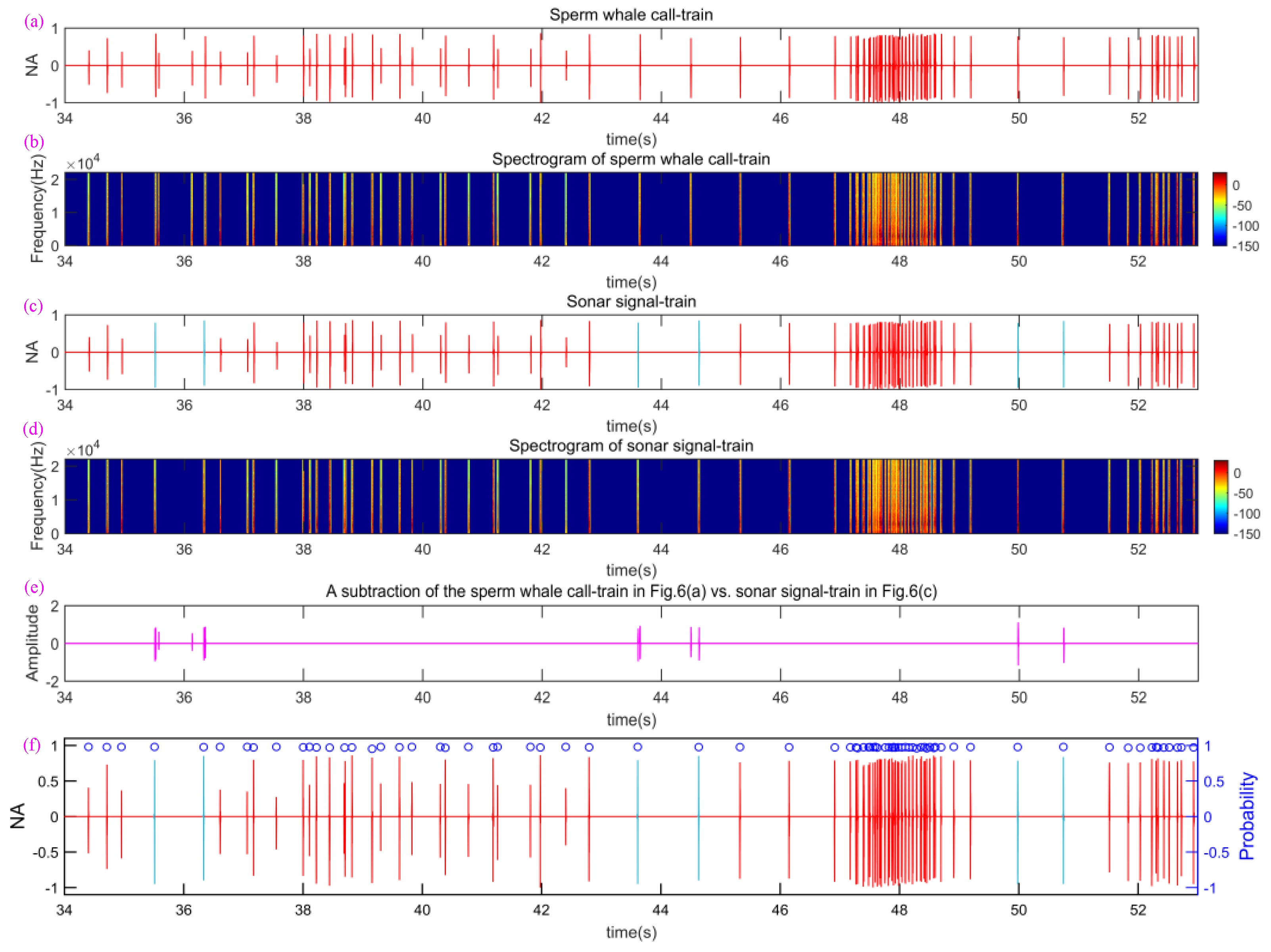
- Because the signal-train transmitted by the active sonar system is composed of the true sperm whale call-train, which is embed by sonar waveforms, the signal-train is very close to the true sperm whale call-train, and thus is difficult to classify into sonar signals rather than a marine mammals’ sound. So the signal-train transmitted by the active sonar system can obtain excellent camouflage ability.
- (4)
- The proposed approach overcomes the trade-off between long-range detection and covertness. It can obtain covertness camouflage even if the SNR of the transmitted signals is very high. On the other hand, it can improve the covertness by reducing the SNR for a short range target detection task.
2. Bio-Inspired Disguised Active Sonar Strategy Based on Sperm Whale Calls
2.1. The Characteristics and Laws of Sperm Whale Call-Train
2.2. Construction of the Disguised Active Sonar Signal-Train
- (1)
- How to effectively filter the ocean noise out and remove the low-energy call pulses from the original sperm whale call-train;
- (2)
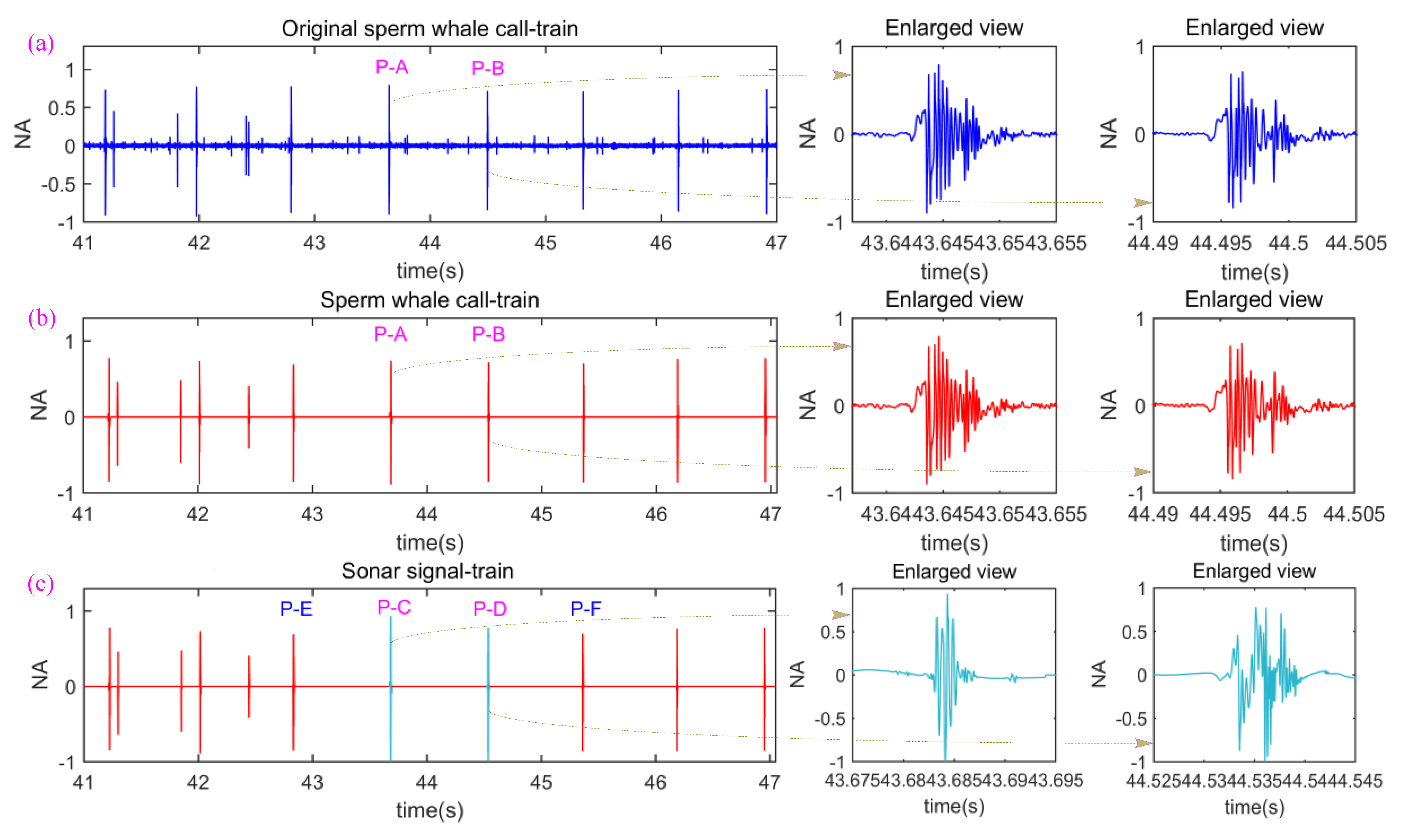
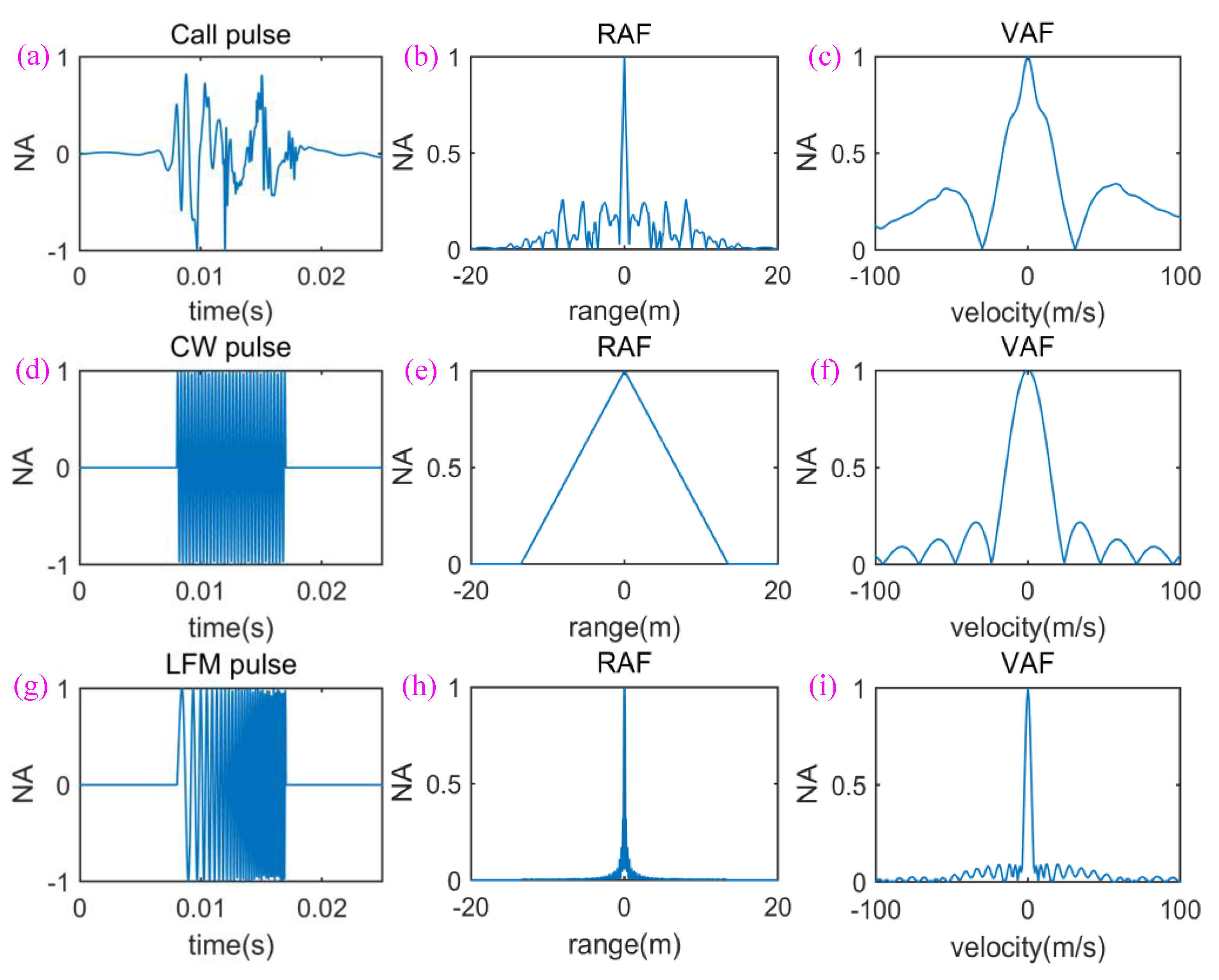
- What characteristics do sperm whale call pulses have from the perspective of serving as sonar signal pulses? Which call pulses are suitable for sonar signal pulses (such as “P-C” and “P-D”)?
- (3)
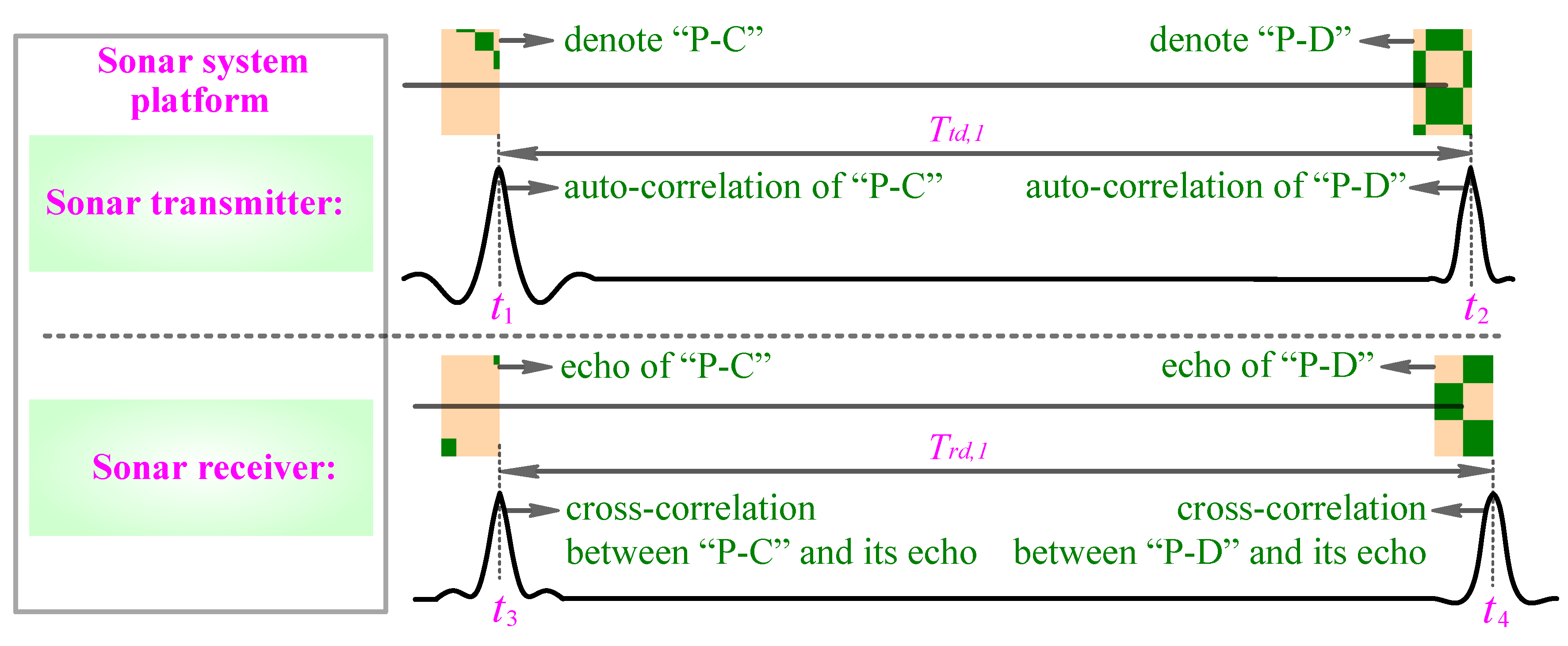
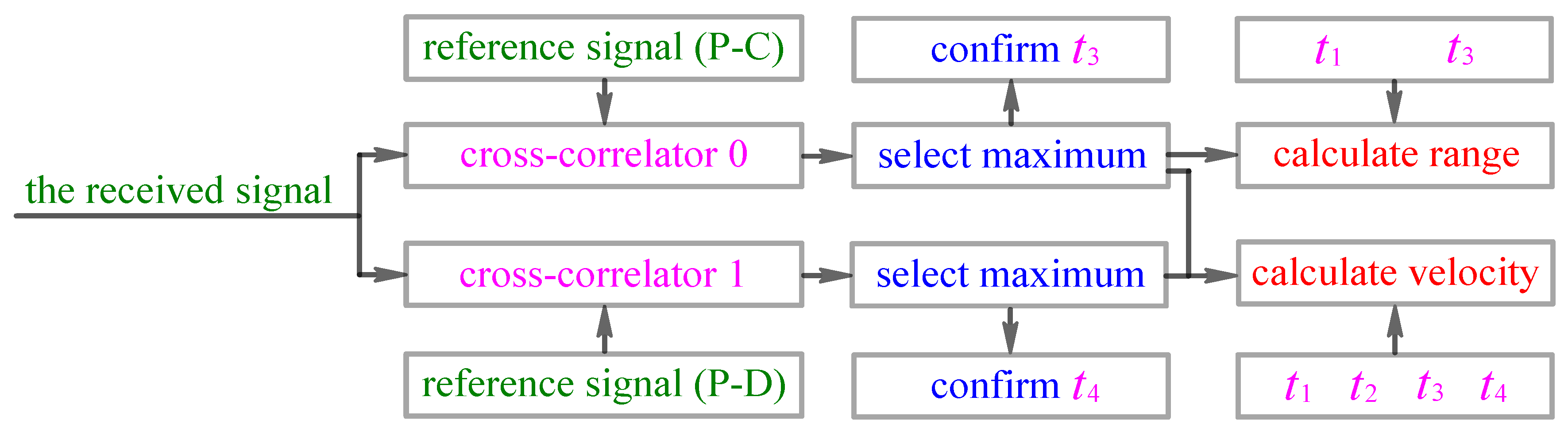
- How to measure the range and velocity of underwater targets using the RVMC;
- (4)
- How to further improve the disguised ability of the constructed active sonar signal-train.
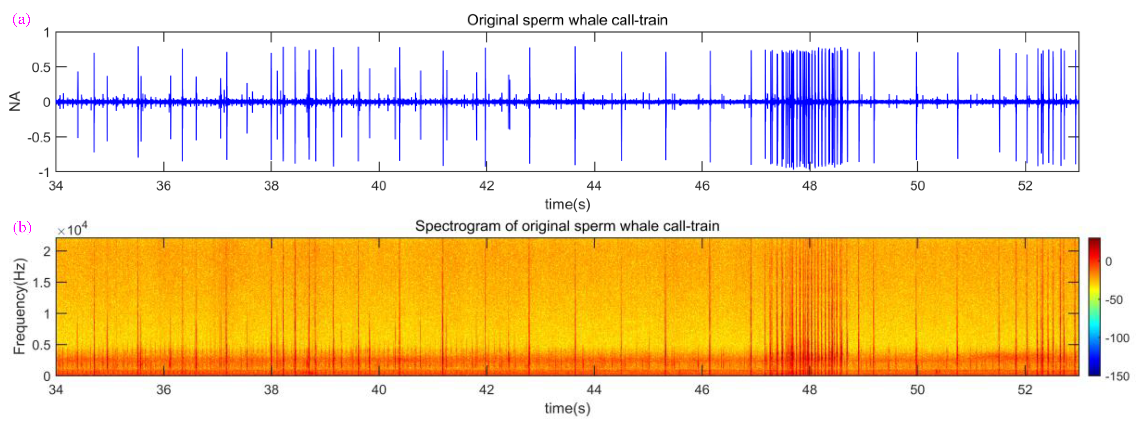
2.3. Preprocessing of the Original Sperm Whale Call-Train
- (1)
- Decompose the mixed signal composed of the ocean noise and sperm whale call-train by using wavelet transform; where and denote the sperm whale call-train and ocean noise, respectively. More specifically, the noise and sperm whale call-train are decomposed into levels by discrete wavelet transform using the symlets wavelet-packet.
- (2)
- Use a soft threshold level given by an estimator developed by David Donoho [37]to shrink the wavelet detailed coefficients of the noise. is the noise standard deviation and is the signal length.
- (3)
- The inverse discrete wavelet transform is used to reconstruct the denoised signal.
- (1)
- (2)
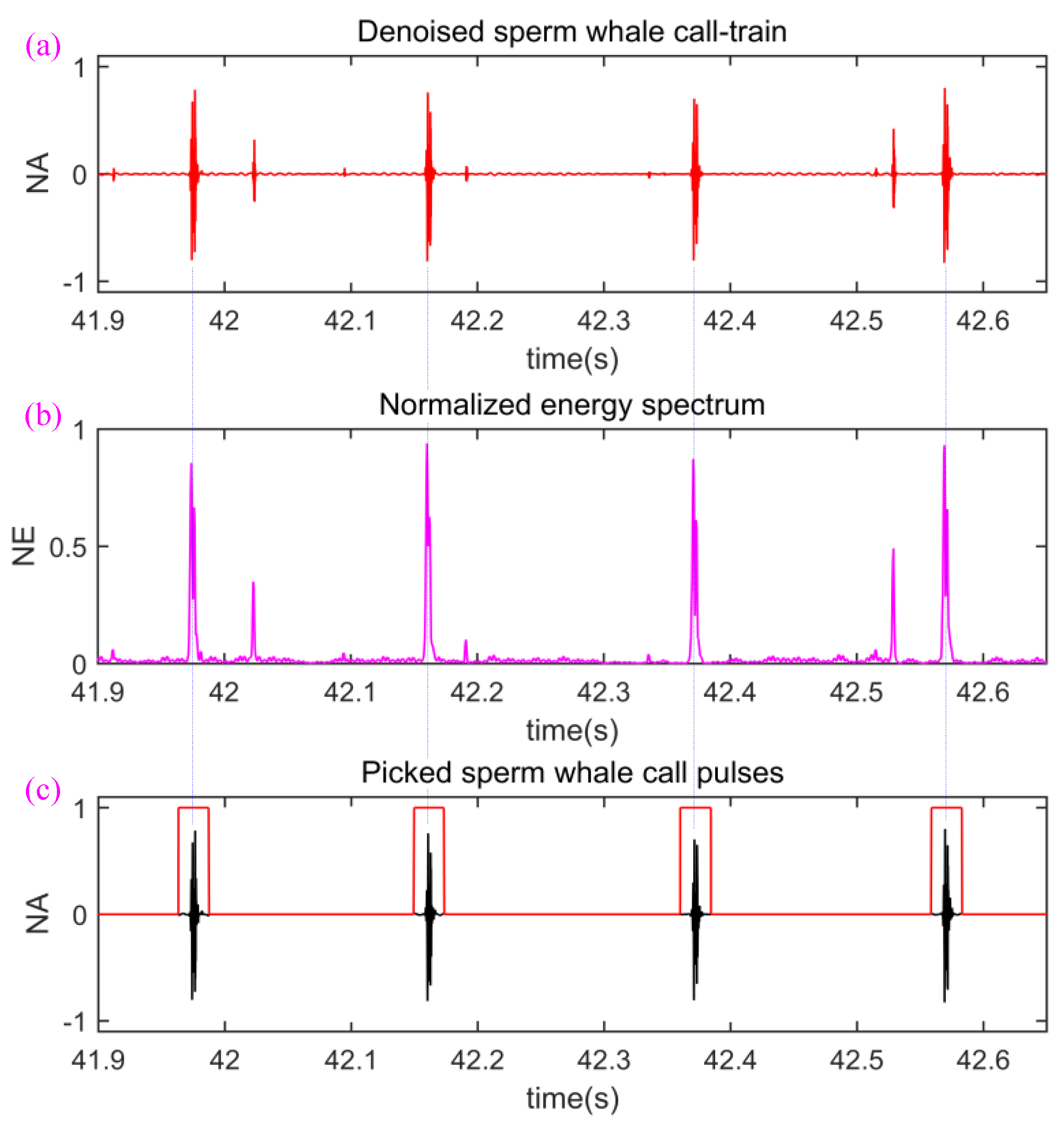
- Next, we set a NE threshold value , then find out all energy peaks which are asked to be more than , and record the locations in time axis corresponding to call energy peaks. For example, when is set to 0.5, the four locations corresponding to four blue dotted lines are recorded in Figure 5.
- (3)
- (4)
- Finally, all rectangle windows are used to perform the AND operation with the sperm whale call-train in Figure 5a. Because the high and low levels of the rectangle windows are “1” and “0” respectively, the low-energy signals containing low-energy call pulses and residual noise was set to “0” and the high-energy call pulses were not changed. In other words, the low-energy signals containing low-energy call pulses and residual noise are removed and the high-energy call pulses are retained, as shown in Figure 5c.
2.4. Analysis and Statistics for Sonar Signal Pulses
2.5. Measurement of Range and Velocity of Underwater Targets
2.6. Improving of the Disguised and Covert Ability
3. Discussions
4. Simulations and Experiments
4.1. Disguised Ability of Constructed Sonar Signal-Train
4.2. Ouput Power Comparison
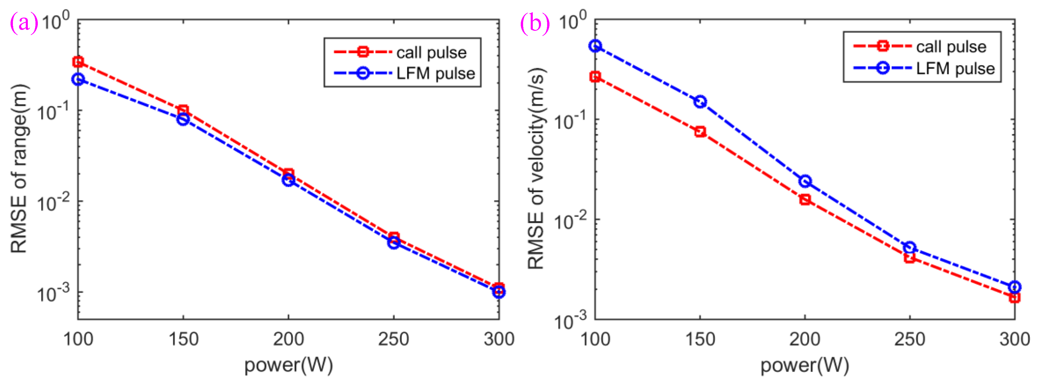
4.3. Efficiency of Underwater Targets Detection
5. Conclusions
Author Contributions
Funding
Acknowledgments
Conflicts of Interest
References
- Zhao, Z.; Zhao, A.; Hui, J.; Hou, B.; Sotudeh, R.; Niu, F. A frequency-domain adaptive matched filter for active sonar detection. Sensors 2017, 17, 1565. [Google Scholar] [CrossRef] [PubMed]
- Zhao, A.; Ma, L.; Ma, X.; Hui, J. An improved azimuth angle estimation method with a single acoustic vector sensor based on an active sonar detection system. Sensors 2017, 17, 412. [Google Scholar] [CrossRef] [PubMed]
- He, B.; Liang, Y.; Feng, X.; Nian, R.; Yan, T.; Li, M.; Zhang, S. AUV SLAM and experiments using a mechanical scanning forward-looking sonar. Sensors 2012, 12, 9386–9410. [Google Scholar] [CrossRef] [PubMed]
- He, B.; Zhang, H.; Li, C.; Zhang, S.; Liang, Y.; Yan, T. Autonomous navigation for autonomous underwater vehicles based on information filters and active sensing. Sensors 2011, 11, 10958–10980. [Google Scholar] [CrossRef] [PubMed]
- Zhang, Z.; Nowak, M.J.; Wicks, M.; Wu, Z. Bio-inspired RF steganography via linear chirp radar signals. IEEE Commun. Mag. 2016, 54, 82–86. [Google Scholar] [CrossRef]
- Nicholson, D.L. Spread Spectrum Signal Design: LPE and AJ Systems; Computer Science Press, Inc.: Rockville, MD, USA, 1988. [Google Scholar]
- Lourey, S.J. Frequency hopping waveforms for continuous active sonar. In Proceedings of the IEEE International Conference on Acoustics, Speech and Signal Processing, Brisbane, Australia, 19–24 April 2015; pp. 1832–1835. [Google Scholar]
- Keerthi, Y.; Bhatt, T.D. LPI radar signal generation and detection. Int. Res. J. Eng. Technol. 2015, 2, 721–727. [Google Scholar]
- Stanciu, M.I.; Azou, S.; Serbanescu, A. On the blind estimation of chip time of time-hopping signals through minimization of a multimodal cost function. IEEE Trans. Signal Process. 2011, 59, 842–847. [Google Scholar] [CrossRef]
- Marszal, J.; Salamon, R. Detection range of intercept sonar for CWFM signals. Arch. Acoust. 2014, 39, 215–230. [Google Scholar] [CrossRef]
- Marszal, J.; Salamon, R.; Kilian, L. Application of maximum length sequence in silent sonar. Hydroacoustics 2012, 15, 143–152. [Google Scholar]
- Marszal, J.; Salamon, R.; Zachariasz, K.; Schmidt, A. Doppler effect in the cw fm sonar. Hydroacoustics 2011, 14, 157–164. [Google Scholar]
- Kulpa, K.; Lukin, K.; Miceli, W.; Thayaparan, T. Signal processing in noise radar technology. IET Radar Sonar Navig. 2008, 2, 229–232. [Google Scholar] [CrossRef]
- Lynch, R.S.; Willett, P.K.; Reinert, J.M. Some analysis of the LPI concept for active sonar. IEEE J. Ocean. Eng. 2012, 37, 446–455. [Google Scholar] [CrossRef]
- Iglesias, V.; Grajal, J.; Royer, P.; Sanchez, M.A.; Lopez-Vallejo, M.; Yeste-Ojeda, O.A. Real-time low-complexity automatic modulation classifier for pulsed radar signals. IEEE Trans. Aerosp. Electron. Syst. 2015, 51, 108–126. [Google Scholar] [CrossRef]
- Shui, P.L.; Bao, Z.; Su, H.T. Nonparametric detection of FM signals using time-frequency ridge energy. IEEE Trans. Signal Process. 2008, 56, 1749–1760. [Google Scholar] [CrossRef]
- Learned, R.E.; Willsky, A.S. A wavelet packet approach to transient signal classification. Appl. Comput. Harmon. Anal. 1995, 12, 265–278. [Google Scholar] [CrossRef]
- Morrissey, R.P.; Ward, J.; DiMarzio, N.; Jarvis, S.; Moretti, D.J. Passive acoustic detection and localization of sperm whales (Physeter macrocephalus) in the tongue of the ocean. Appl. Acoust. 2006, 67, 1091–1105. [Google Scholar] [CrossRef]
- Wu, L.; Babu, P.; Palomar, D.P. Transmit waveform/receive filter design for MIMO radar with multiple waveform constraints. IEEE Trans. Signal Process. 2017, 66, 1526–1540. [Google Scholar] [CrossRef]
- Tang, B.; Naghsh, M.M.; Tang, J. Relative entropy-based waveform design for MIMO radar detection in the presence of clutter and interference. IEEE Trans. Signal Process. 2015, 63, 3783–3796. [Google Scholar] [CrossRef]
- Cheng, Z.; He, Z.; Zhang, S.; Li, J. Constant modulus waveform design for MIMO radar transmit beampattern. IEEE Trans. Signal Process. 2017, 65, 4912–4923. [Google Scholar] [CrossRef]
- Mueller, R.; Kuc, R. Biosonar-inspired technology: Goals, challenges and insights. Bioinspir. Biomim. 2007, 2, 146–161. [Google Scholar] [CrossRef] [PubMed]
- Capus, C.; Pailhas, Y.; Brown, K.; Lane, D.M.; Moore, P.W.; Houser, D. Bio-inspired wideband sonar signals based on observations of the bottlenose dolphin (Tursiops truncatus). J. Acoust. Soc. Am. 2007, 121, 594–604. [Google Scholar] [CrossRef] [PubMed]
- Hurtado, M.; Nehorai, A. Bat-inspired adaptive design of waveform and trajectory for radar. In Proceedings of the IEEE Asilomar Conference on Signals, Systems and Computers, Pacific Grove, CA, USA, 26–29 October 2008; pp. 36–40. [Google Scholar]
- Vespe, M.; Jones, G.; Bakers, C.J. Lessons for radar waveform diversity in echolocating mammals. IEEE Signal Process. Mag. 2009, 26, 65–75. [Google Scholar] [CrossRef]
- Amichai, E.; Blumrosen, G.; Yovel, Y. Calling louder and longer: How bats use biosonar under severe acoustic interference from other bats. Proc. Biol. Sci. 2015, 282, 1821. [Google Scholar] [CrossRef] [PubMed]
- Van IJsselmuide, S.P.; Beerens, S.P. Detection and classification of marine mammals using an LFAS system. J. Thorac. Oncol. 2004, 32, 417–424. [Google Scholar]
- Chin-Hsing, C.; Jiann-Der, L.; Ming-Chi, L. Classification of underwater signals using wavelet transforms and neural networks. Math. Comput. Model. 1998, 27, 47–60. [Google Scholar] [CrossRef]
- Papandreou-Suppappola, A.; Suppappola, S.B. Analysis and classification of time-varying signals with multiple time-frequency structures. IEEE Signal Process. Lett. 2015, 9, 92–95. [Google Scholar] [CrossRef]
- Wahlberg, M.; Frantzis, A.; Alexiadou, P.; Madsen, P.T.; Møhl, B. Click production during breathing in a sperm whale (Physeter macrocephalus). J. Acoust. Soc. Am. 2005, 118, 3404–3407. [Google Scholar] [CrossRef] [PubMed]
- Zimmer, W.M.X.; Tyack, P.L.; Johnson, M.P.; Madsen, P.T. Three-dimensional beam pattern of regular sperm whale clicks confirms bent-horn hypothesis. J. Acoust. Soc. Am. 2005, 117, 1473–1485. [Google Scholar] [CrossRef] [PubMed]
- Andre, M.; Kamminga, C. Rhythmic dimension in the echolocation click trains of sperm whales: A possible function of identification and communication. J. Mar. Biol. Assoc. UK 2000, 80, 163–169. [Google Scholar] [CrossRef]
- Jaquet, N.; Dawson, S.; Douglas, L. Vocal behavior of male sperm whales: Why do they click? J. Acoust. Soc. Am. 2001, 109, 2254–2259. [Google Scholar] [CrossRef] [PubMed]
- Nosal, E.M.; Frazer, L.N. Track of a sperm whale from delays between direct and surface-reflected clicks. Appl. Acoust. 2006, 67, 1187–1201. [Google Scholar] [CrossRef]
- The Data Source Used in This Paper. Available online: http://macaulaylibrary.org/search?media_collection=1&taxon_id=10530453&taxon_rank_id=55&q=Sperm+Whales (accessed on 26 July 2018).
- Peng, Z.K.; Chu, F.L. Application of the wavelet transform in machine condition monitoring and fault diagnostics: A review with bibliography. Mech. Syst. Signal Process. 2004, 18, 199–221. [Google Scholar] [CrossRef]
- Donoho, D.L. De-noising by soft-thresholding. IEEE Trans. Inf. Theory 1995, 41, 613–627. [Google Scholar] [CrossRef]
- Wilpon, J.G.; Rabiner, L.R.; Martin, T. An improved word-detection algorithm for telephone-quality speech incorporating both syntactic and semantic constraints. Bell Lab. Tech. J. 1984, 63, 479–498. [Google Scholar] [CrossRef]
- Pecknold, S.P.; Renaud, W.M.; McGaughey, D.R.; Theriault, J.A.; Marsden, R.F. Improved active sonar performance using Costas waveforms. IEEE J. Ocean. Eng. 2009, 34, 559–574. [Google Scholar] [CrossRef]
- Benedetto, J.J.; Konstantinidis, I.; Rangaswamy, M. Phase-coded waveforms and their design. IEEE Signal Process. Mag. 2009, 26, 22–31. [Google Scholar] [CrossRef]
- Wang, W.Q. MIMO SAR chirp modulation diversity waveform design. IEEE Geosci. Remote Sens. Lett. 2014, 11, 1644–1648. [Google Scholar] [CrossRef]
- Phillips, A.B.; Turnock, S.R.; Furlong, M. The use of computational fluid dynamics to aid cost-effective hydrodynamic design of autonomous underwater vehicles. J. Eng. Marit. Environ. 2010, 224, 1–16. [Google Scholar] [CrossRef]
- Jun, B.H.; Park, J.Y.; Lee, F.Y.; Lee, P.M.; Lee, C.M.; Kim, K.; Lim, Y.K.; Oh, J.H. Development of the AUV ‘ISiMI’ and a free running test in an ocean engineering basin. Ocean Eng. 2009, 36, 2–14. [Google Scholar] [CrossRef]
- Bellingham, J.G.; Zhang, Y.; Kerwin, J.E.; Erikson, J.; Hobson, B.; Kieft, B.; Godin, M.; McEwen, R.; Hoover, T.; Paul, J.; et al. Efficient propulsion for the Tethys long-range autonomous underwater vehicle. IEEE Ocean. Eng. Soc. Newsl. 2010, 3, 1–7. [Google Scholar]
- Miasnikov, E. What is known about the character of noise created by submarines? In The Future of Russia’s Strategic Nuclear Forces: Discussions and Arguments; The Center For Arms Control, Energy, and Environmental Studies: at Moscow Institute of Physics and Technology: Dolgoprudny, Russia, 1998; Available online: https://fas.org/spp/eprint/snf03221.htm (accessed on 26 July 2018).
- Ghosh, J.; Deuser, L.; Beck, S.D. A neural network based hybrid system for detection, characterization, and classification of short-duration oceanic signals. IEEE J. Ocean. Eng. 1992, 17, 351–363. [Google Scholar] [CrossRef]
- Huynh, Q.Q.; Cooper, L.N.; Intrator, N.; Shouval, H. Classification of underwater mammals using feature extraction based on time-frequency analysis and BCM theory. IEEE Trans. Signal Process. 1998, 46, 1202–1207. [Google Scholar] [CrossRef]
- Lee, D.H.; Shin, J.W.; Do, D.W.; Choi, S.M.; Kim, H.N. Robust LFM target detection in wideband sonar systems. IEEE Trans. Aerosp. Electron. Syst. 2017, 53, 2399–2412. [Google Scholar] [CrossRef]
- Pecknold, S.; Theriault, J.A.; McGaughey, D.; Collins, J. Time-series modeling using the waveform transmission through a channel program. In Proceedings of the Europe Oceans 2005, Brest, France, 20–23 June 2005; Volume 2, pp. 993–1000. [Google Scholar]
- Porter, M.B. The Bellhop Manual and Users Guide: Preliminary draft; Technical Report; Heat, Light, and Sound Research, Inc.: La Jolla, CA, USA, 2011. [Google Scholar]
- Mccammon, D. Active acoustics using Bellhop-DRDC: Run time tests and suggested configurations for a tracking exercise in shallow scotian waters. Arch. Biochem. Biophys. 2005, 68, 507–509. [Google Scholar]
- Jensen, F. Numerical models of sound propagation in real oceans. In Proceedings of the Oceans IEEE, Washington, DC, USA, 20–22 September 1982; pp. 147–154. [Google Scholar]
- Hickman, G.; Krolik, J.L. Matched-field depth estimation for active sonar. J. Acoust. Soc. Am. 2004, 115, 620–629. [Google Scholar] [CrossRef] [PubMed]


| RR (m) or(ms) | Number | VR (m/s) or DT | Number | |
| RR 1.50 or 1.000 | 863 | VR 1.0 or DT 0.0013 | 0 | |
| RR 1.00 or 0.667 | 839 | VR 2.0 or DT 0.0027 | 16 | |
| RR 0.50 or 0.333 | 620 | VR 3.0 or DT 0.0040 | 198 | |
| RR 0.10 or 0.067 | 495 | VR 4.0 or DT 0.0053 | 812 | |
| RR 0.05 or 0.033 | 77 | VR 5.0 or DT 0.0067 | 863 | |
| Group | Threshold value | Number | ||
| 1 | {RR 1.0 m, VR 3.0 m/s} or { 0.667 ms, DT 0.0040} | 189 | ||
| 2 | {RR 1.0 m, VR 2.5 m/s} or { 0.667 ms, DT 0.0033} | 46 | ||
| 3 | {RR 1.0 m, VR 2.0 m/s} or { 0.667 ms, DT 0.0027} | 2 | ||
| 4 | {RR 0.5 m, VR 2.0 m/s} or { 0.333 ms, DT 0.0027} | 0 | ||
| 5 | {RR 1.5 m, VR 1.0 m/s} or { 1.000 ms, DT 0.0013} | 0 | ||
| RR (m) or (ms) | Number | VR (m/s) or DT | Number | |
|---|---|---|---|---|
| RR 1.50 or 1.000 | 863 | VR 2.0 or DT 0.0027 | 833 | |
| RR 1.00 or 0.667 | 839 | VR 2.5 or DT 0.0033 | 607 | |
| RR 0.50 or 0.333 | 620 | VR 3.0 or DT 0.0040 | 308 | |
| RR 0.10 or 0.067 | 495 | VR 3.5 or DT 0.0047 | 178 | |
| RR 0.05 or 0.033 | 77 | VR 4.0 or DT 0.0053 | 65 | |
| Group | Threshold value | Number | ||
| 1 | {RR 1.5 m, VR 4.0 m/s } or { 1.000 ms, DT 0.0053} | 65 | ||
| 2 | {RR 1.5 m, VR 3.5 m/s} or { 1.000 ms, DT 0.0047} | 178 | ||
| 3 | {RR 1.0 m, VR 3.5 m/s} or { 0.667 ms, DT 0.0047} | 170 | ||
| 4 | {RR 0.5 m, VR 3.5 m/s} or { 0.333 ms, DT 0.0047} | 102 | ||
| 5 | {RR 0.1 m, VR 3.5 m/s} or { 0.067 ms, DT 0.0047} | 86 | ||
| 6 | {RR 0.1 m, VR 3.0 m/s} or { 0.067 ms, DT 0.0040} | 52 | ||
© 2018 by the authors. Licensee MDPI, Basel, Switzerland. This article is an open access article distributed under the terms and conditions of the Creative Commons Attribution (CC BY) license (http://creativecommons.org/licenses/by/4.0/).
Share and Cite
Jiang, J.; Wang, X.; Duan, F.; Li, C.; Fu, X.; Huang, T.; Bu, L.; Ma, L.; Sun, Z. Bio-Inspired Covert Active Sonar Strategy. Sensors 2018, 18, 2436. https://doi.org/10.3390/s18082436
Jiang J, Wang X, Duan F, Li C, Fu X, Huang T, Bu L, Ma L, Sun Z. Bio-Inspired Covert Active Sonar Strategy. Sensors. 2018; 18(8):2436. https://doi.org/10.3390/s18082436
Chicago/Turabian StyleJiang, Jiajia, Xianquan Wang, Fajie Duan, Chunyue Li, Xiao Fu, Tingting Huang, Lingran Bu, Ling Ma, and Zhongbo Sun. 2018. "Bio-Inspired Covert Active Sonar Strategy" Sensors 18, no. 8: 2436. https://doi.org/10.3390/s18082436
APA StyleJiang, J., Wang, X., Duan, F., Li, C., Fu, X., Huang, T., Bu, L., Ma, L., & Sun, Z. (2018). Bio-Inspired Covert Active Sonar Strategy. Sensors, 18(8), 2436. https://doi.org/10.3390/s18082436