A Parameter Self-Calibration Method for GNSS/INS Deeply Coupled Navigation Systems in Highly Dynamic Environments

Abstract
1. Introduction
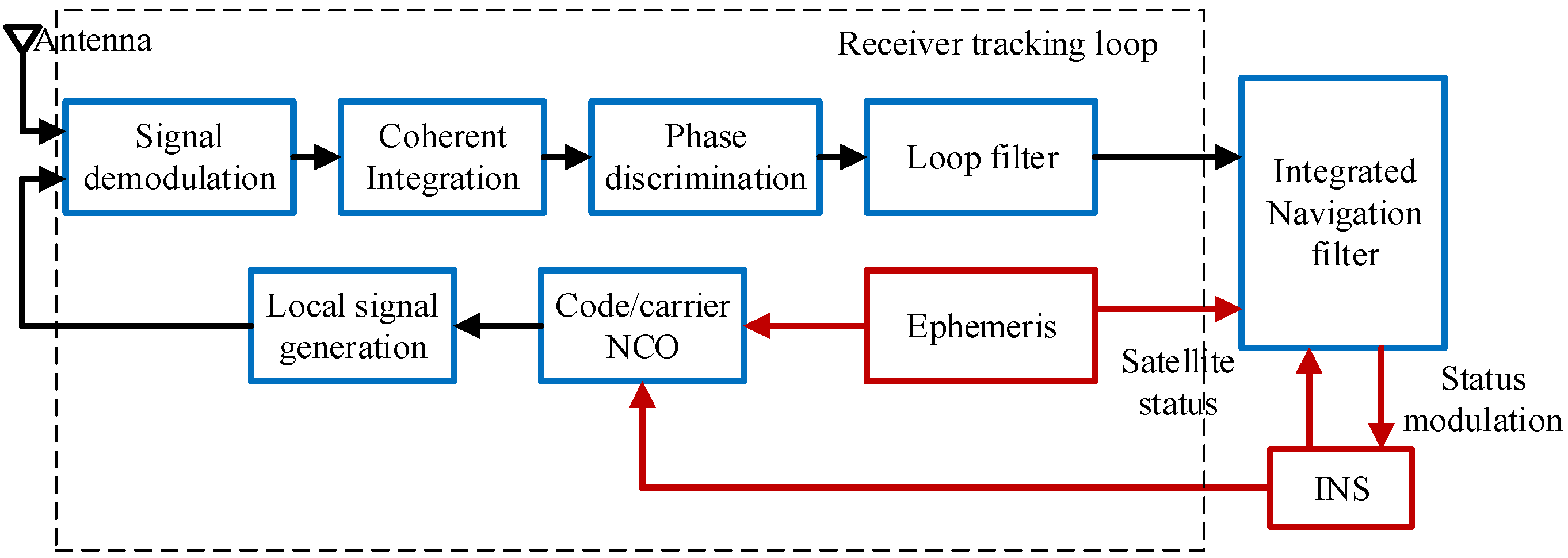
2. Mathematical Model of a Deeply Coupled Navigation System
3. Parameter Self-Calibration Method for Loops in Deeply Coupled Systems Based on Norm Analysis
3.1. Norm Analysis to the IMU Error Propagation Properties
- (1)
- ; further, if, and only if, . (Positive-definiteness)
- (2)
- for any scalar . (Homogeneity)
- (3)
- . (Triangle inequality)
3.2. Parameter Self-Calibration Method for the Tracking Loop in a Deeply Coupled System
4. Highly Dynamic Simulations and Results
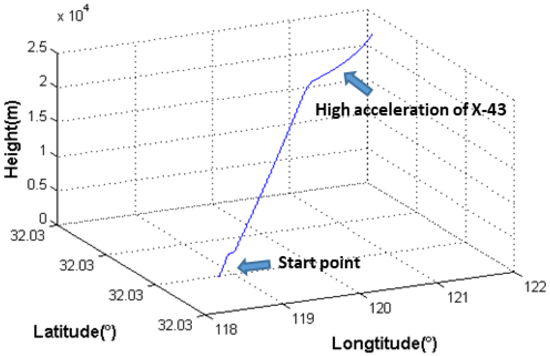
4.1. Simulation Conditions and Track Settings
4.2. Simulation of Inertial Calculation
4.2.1. Norm Analysis Simulation
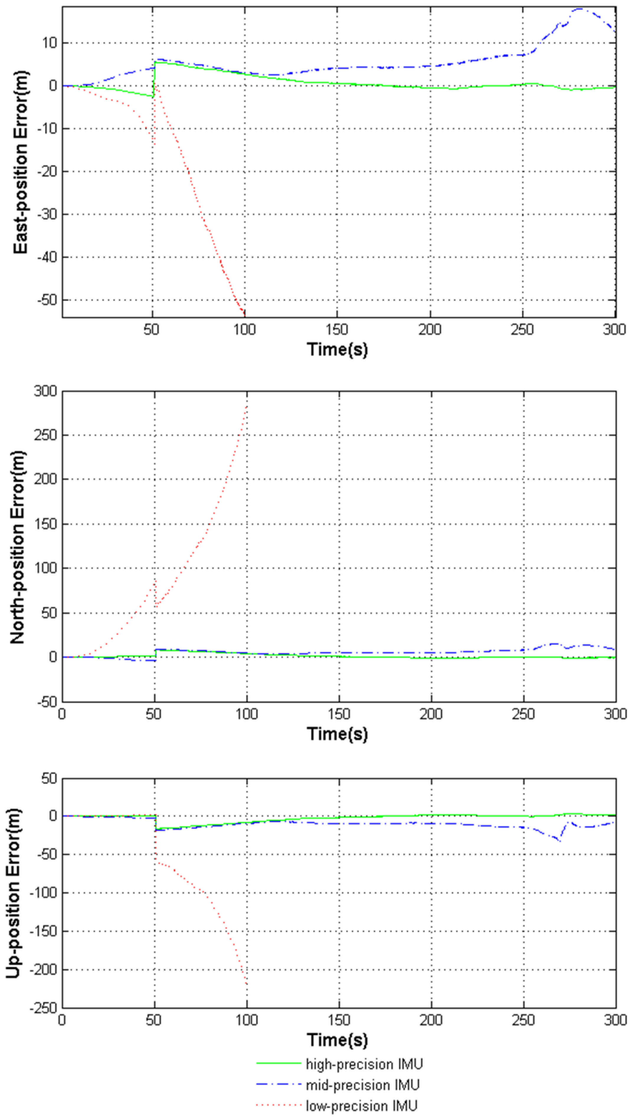
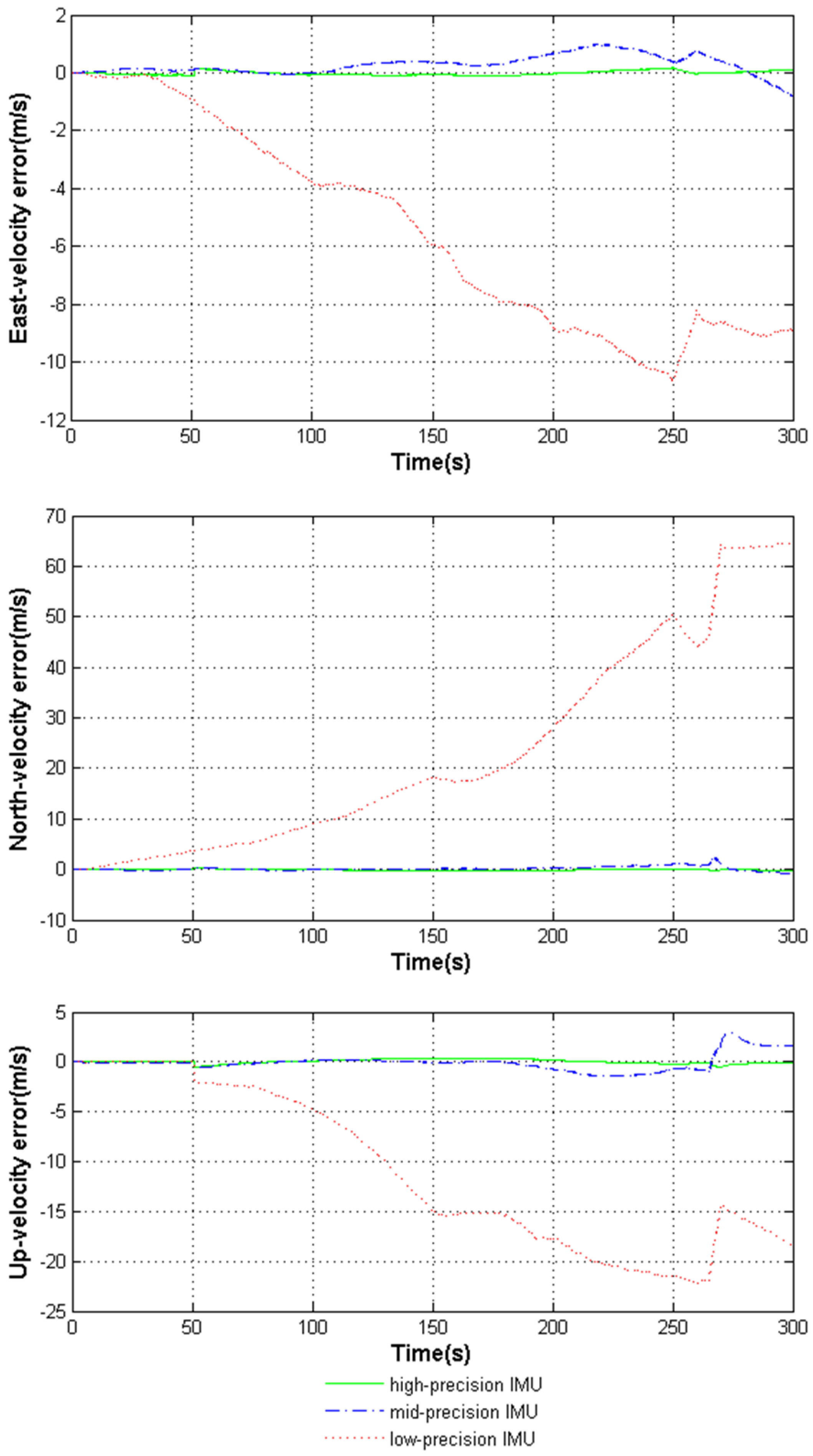
4.2.2. Stability Simulation under Highly Dynamic Circumstances
5. Conclusions
Author Contributions
Funding
Conflicts of Interest
References
- Zhang, T.; Niu, X.; Ban, Y.; Zhang, H.; Shi, C.; Liu, J. Modeling and development of INS-aided PLLs in a GNSS/INS deeply-coupled hardware prototype for dynamic applications. Sensors 2015, 15, 733–759. [Google Scholar] [CrossRef] [PubMed]
- Liu, G.; Guo, M.; Zhang, R.; Peng, Z.; Luo, S. MIMU precision’s influence on GNSS/MINS integrated navigation system performance by simulation analysis. J. Chin. Inert. Technol. 2013, 21, 786–791. [Google Scholar]
- Zeng, Q.; Meng, Q.; Liu, J.; Feng, S.; Wang, H. Acquisition and loop control of ultra-tight INS/BeiDou integration system. Optik 2016, 127, 8082–8089. [Google Scholar] [CrossRef]
- Kirkko-Jaakkola, M.; Ruotsalainen, L.; Bhuiyan, M.Z.H.; Soderholm, S.; Thombre, S.; Kuusniemi, H. Performance of a MEMS IMU Deeply Coupled with a GNSS Receiver under Jamming. In Proceedings of the Ubiquitous Positioning Indoor Navigation and Location Based Service (UPINLBS), Corpus Christi, TX, USA, 20–21 November 2014. [Google Scholar]
- Adeel, M.; Chen, X.; Yu, W.; Ying, R.; Liu, P. Performance Analysis of Deeply Coupled INS Assisted Multi-Carrier Vector Phase Lock Loop for High Dynamics. In Proceedings of the 28th International Technical Meeting of The Satellite-Division-of-the-Institute-of-Navigation (ION GNSS+), Tampa, FL, USA, 14–18 September 2015. [Google Scholar]
- Langer, M.; Trommer, G.F. Multi GNSS constellation deeply coupled GNSS/INS integration for automotive application using a software defined GNSS receiver. In Proceedings of the 2014 IEEE/ION Position, Location and Navigation Symposium (PLANS 2014), Monterey, CA, USA, 5–8 May 2014; pp. 1105–1112. [Google Scholar]
- Slater, C.; Creaghan, M.; Lamce, O. Six-Axis Monopropellant Propulsion System for Picosatellites; Massachusetts Instritute of Technology Press: Cambridge, MA, USA, 2016; p. 39. [Google Scholar]
- Chen, Z. Analysis of the IMU precision’s influence on the loop of deeply-coupled GNSS/INS navigation system in high-dynamic environment. Optik 2016, 127, 11379–11385. [Google Scholar] [CrossRef]
- Bancroft, J.B.; Lachapelle, G. Estimating MEMS Gyroscope G-Sensitivity Errors in foot mounted navigation. In Proceedings of the Ubiquitous Positioning, Indoor Navigation, and Location Based Service (UPINLBS), Helsinki, Finland, 3–4 October 2012. [Google Scholar]
- Qin, F.; Zhan, X.; Zhan, L. Performance assessment of a low-cost inertial measurement unit based ultra-tight global navigation satellite system/inertial navigation system integration for high dynamic applications. IET Radar Sonar Navig. 2014, 8, 828–836. [Google Scholar] [CrossRef]
- Zeng, Q.; Chen, W.; Liu, J.; Wang, H. An Improved Multi-Sensor Fusion Navigation Algorithm Based on the Factor Graph. Sensors 2017, 17, 641. [Google Scholar] [CrossRef] [PubMed]
- Wagner, J.F. GNSS/INS integration: Still an attractive candidate for automatic landing systems? GPS Solut. 2015, 9, 179–193. [Google Scholar] [CrossRef]
- Xing, L.; Hang, Y.; Xiong, Z.; Liu, J.; Wan, Z. Accurate Attitude Estimation Using ARS under Conditions of Vehicle Movement Based on Disturbance Acceleration Adaptive Estimation and Correction. Sensors 2016, 16, 1726. [Google Scholar] [CrossRef] [PubMed]
- Xie, G. Principles of GPS and Receiver Design; Publishing House of Electronics Industry: Beijing, China, 2009. [Google Scholar]
- Xie, F.; Liu, J.; Li, R.; Jiang, B.; Qiao, L. Performance analysis of a federated ultra-tight global positioning system/inertial navigation system integration algorithm in high dynamic environments. Proc. Inst. Mech. Eng. Part G 2015, 229, 56–71. [Google Scholar] [CrossRef]


| Gyros ID | Bias Repeatability (°/s) | White Noise (°/s) | g-Sensitivity (°/s/g) | 50 g-Sensitivity (°/s) |
|---|---|---|---|---|
| ADIS16490 | 0.05 | 0.05 | 0.005 | 0.25 |
| ADIS16448 | 0.50 | 0.27 | 0.015 | 0.75 |
| ADIS16300 | 2.00 | 1.10 | 0.050 | 2.50 |
| Movement State | Time (s) | Forward Acceleration (m/s/s) | Pitch Rate (°/s) | Final Velocity (m/s) |
|---|---|---|---|---|
| Accelerative running | 0–20 | 4.00 | 0 | 80.000 |
| Accelerative taking-off | 20–35 | 1.00 | 1 | 95.000 |
| Accelerative climbing | 35–75 | 2.00 | 0 | 175.00 |
| Steady climbing | 75–100 | 0 | 0 | 175.00 |
| Change to level flight | 100–115 | 0 | −1 | 175.00 |
| Steady level flight | 115–145 | 0 | 0 | 175.00 |
| Separation from carrier | 145–150 | 0.68 | 0 | 178.40 |
| Ignition of the rocket | 150–153 | 10.0 | 0 | 208.40 |
| Accelerative head-up | 153–163 | 19.0 | 1 | 398.40 |
| Accelerative climbing | 163–250 | 19.0 | 0 | 2051.4 |
| Change to level flight | 250–260 | 0 | −1 | 2051.4 |
| Quick popup of X-43 | 260–265 | 19.0 | 0 | 2146.4 |
| High acceleration of X-43 | 265–270 | 300 | 0 | 3646.4 |
| Steady level flight | 270–300 | 0 | 0 | 3646.4 |
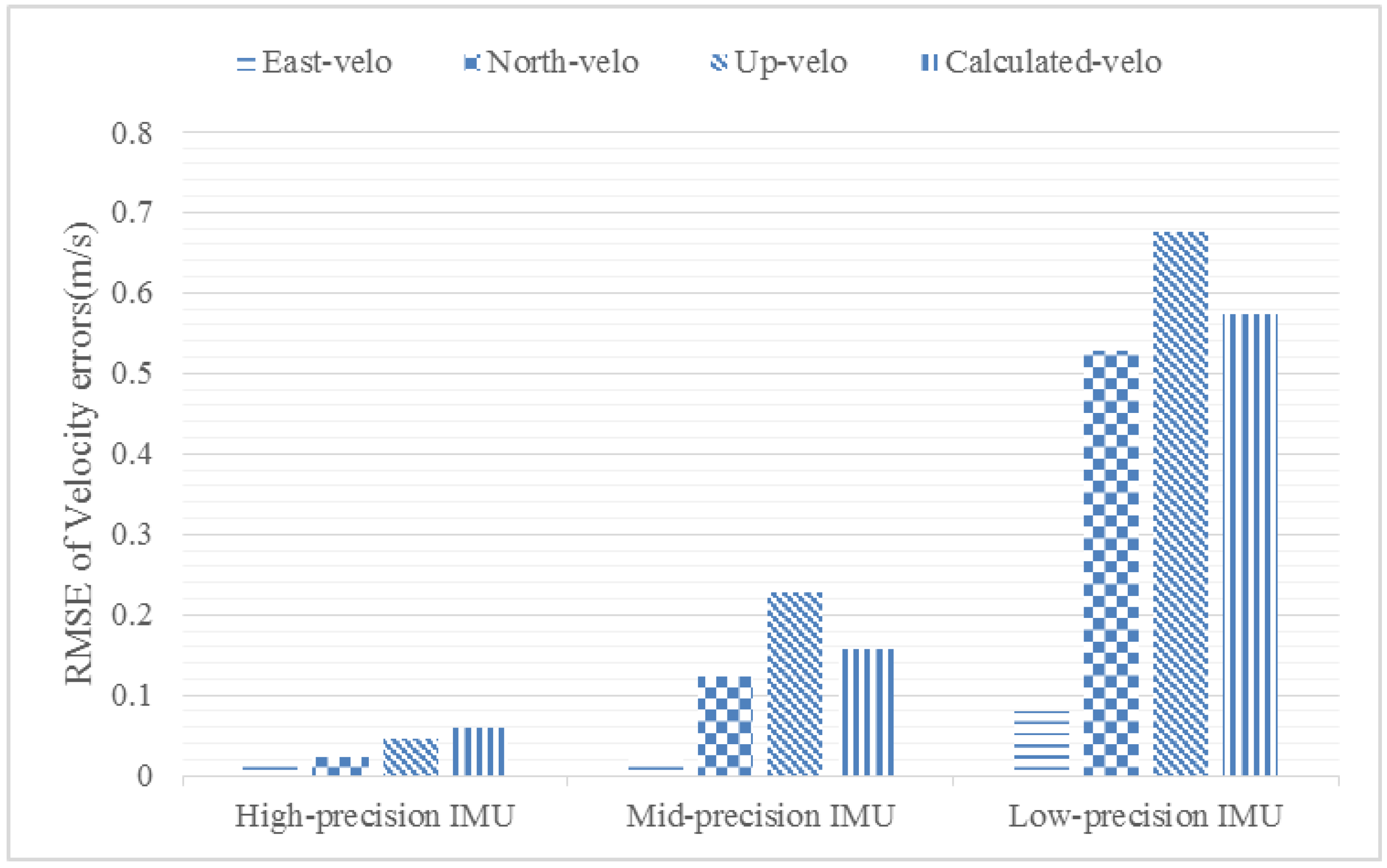
| RMSE of Velocity Errors | High-Precision IMU | Mid-Precision IMU | Low-Precision IMU |
|---|---|---|---|
| East | 0.0150 | 0.0206 | 0.0805 |
| North | 0.0222 | 0.1241 | 0.5268 |
| Up | 0.0456 | 0.2267 | 0.6751 |
| Calculated by Equation (28) | 0.0601 | 0.1574 | 0.5724 |
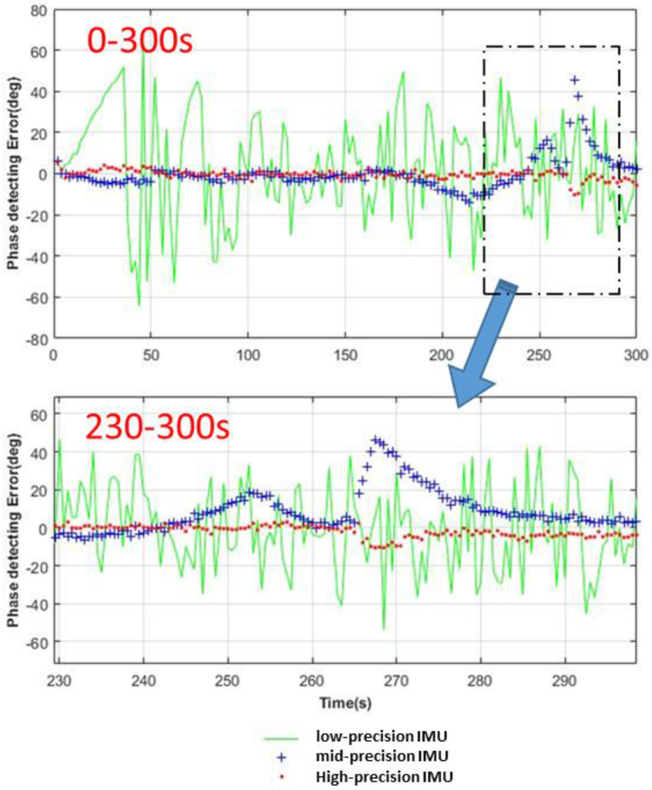
| IMUs | Calculated Phase Error (°) |
|---|---|
| High-precision | 5.08280 (<15) |
| Mid-precision | 11.7625 (<15) |
| Low-precision | 34.1919 (>15) |
| RMSE of System Errors | High-Precision | Mid-Precision | Low-Precision |
|---|---|---|---|
| East-position (m) | 1.9686 | 7.0726 | 407.51 |
| North-position (m) | 2.8281 | 6.9240 | 279.73 |
| Up-position (m) | 5.5569 | 11.482 | 210.98 |
| East-velocity (m/s) | 0.0740 | 0.4287 | 6.5085 |
| North-velocity (m/s) | 0.1307 | 0.4583 | 30.695 |
| Up-velocity (m/s) | 0.2115 | 0.8553 | 13.535 |
© 2018 by the authors. Licensee MDPI, Basel, Switzerland. This article is an open access article distributed under the terms and conditions of the Creative Commons Attribution (CC BY) license (http://creativecommons.org/licenses/by/4.0/).
Share and Cite
Chen, Z.; Lai, J.; Liu, J.; Li, R.; Ji, G. A Parameter Self-Calibration Method for GNSS/INS Deeply Coupled Navigation Systems in Highly Dynamic Environments. Sensors 2018, 18, 2341. https://doi.org/10.3390/s18072341
Chen Z, Lai J, Liu J, Li R, Ji G. A Parameter Self-Calibration Method for GNSS/INS Deeply Coupled Navigation Systems in Highly Dynamic Environments. Sensors. 2018; 18(7):2341. https://doi.org/10.3390/s18072341
Chicago/Turabian StyleChen, Zang, Jizhou Lai, Jianye Liu, Rongbing Li, and Guotian Ji. 2018. "A Parameter Self-Calibration Method for GNSS/INS Deeply Coupled Navigation Systems in Highly Dynamic Environments" Sensors 18, no. 7: 2341. https://doi.org/10.3390/s18072341
APA StyleChen, Z., Lai, J., Liu, J., Li, R., & Ji, G. (2018). A Parameter Self-Calibration Method for GNSS/INS Deeply Coupled Navigation Systems in Highly Dynamic Environments. Sensors, 18(7), 2341. https://doi.org/10.3390/s18072341