Differential Ultra-Wideband Microwave Imaging: Principle Application Challenges


Abstract
1. Introduction
- multipath signals caused by scattering at dominant objects overpowering the reflections of weak bodies;
- device internal clutter, caused by imperfections of the measurement equipment (which can only be suppressed up to a certain degree by appropriate device calibration);
- time extension of the sounding waves due to the limited decay rate of the antenna impulse response; and
- receiver noise, propagation loss, and others.
- temporal fluctuations inherently connected with the test scenario (e.g., the vital motion of inner organs of humans and animals, the breathing motion of buried survivors after an earthquake, and the motion of wood-destroying insects, as well as slowly running events, such as the putrefaction of biological substances, the healing process after a medical surgery [6], post-event monitoring of stroke [7], and many more);
- a targeted influence of the hidden object of interest via modification of its position in space, its volume, and its permittivity or permeability (e.g., the targeting of malignant tissue by nanoparticles, permittivity variation by local heating or cooling [8,9], water accumulation in hygroscopic substances, etc.); and
- small deviations between two largely identical SUTs (cancer in one of the two female breasts [10], foreign objects in chocolate, other identical food pieces, etc.).
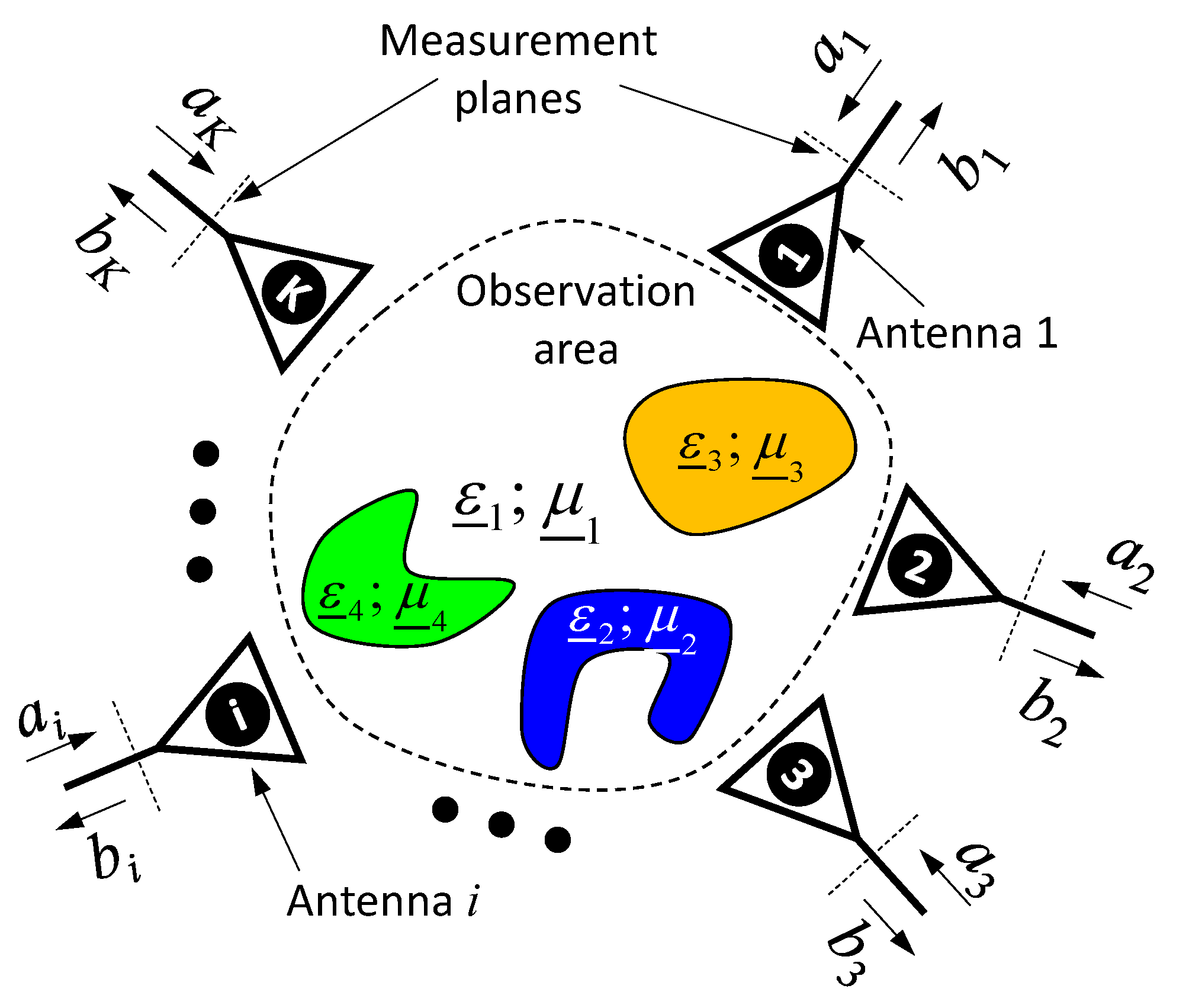
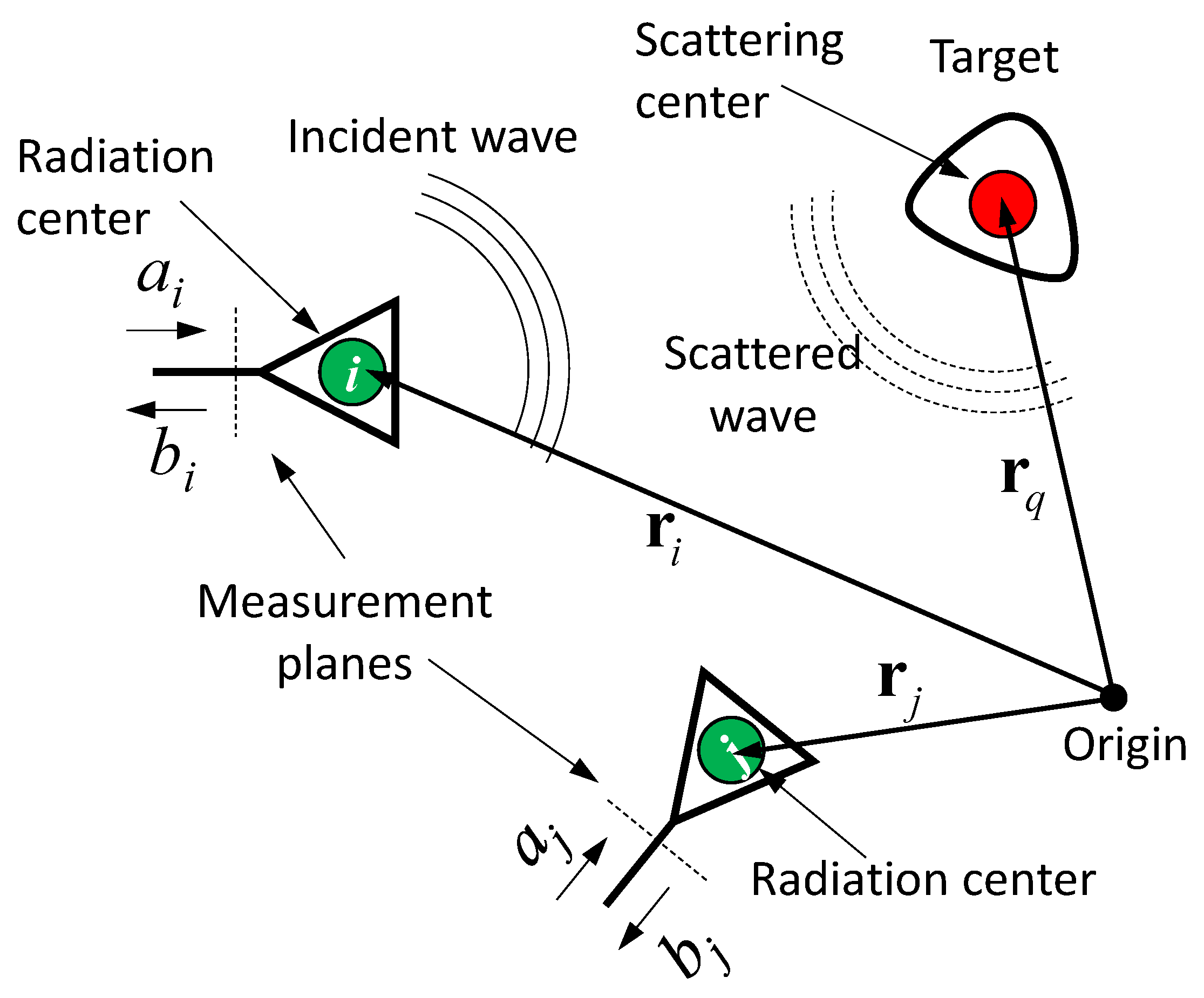
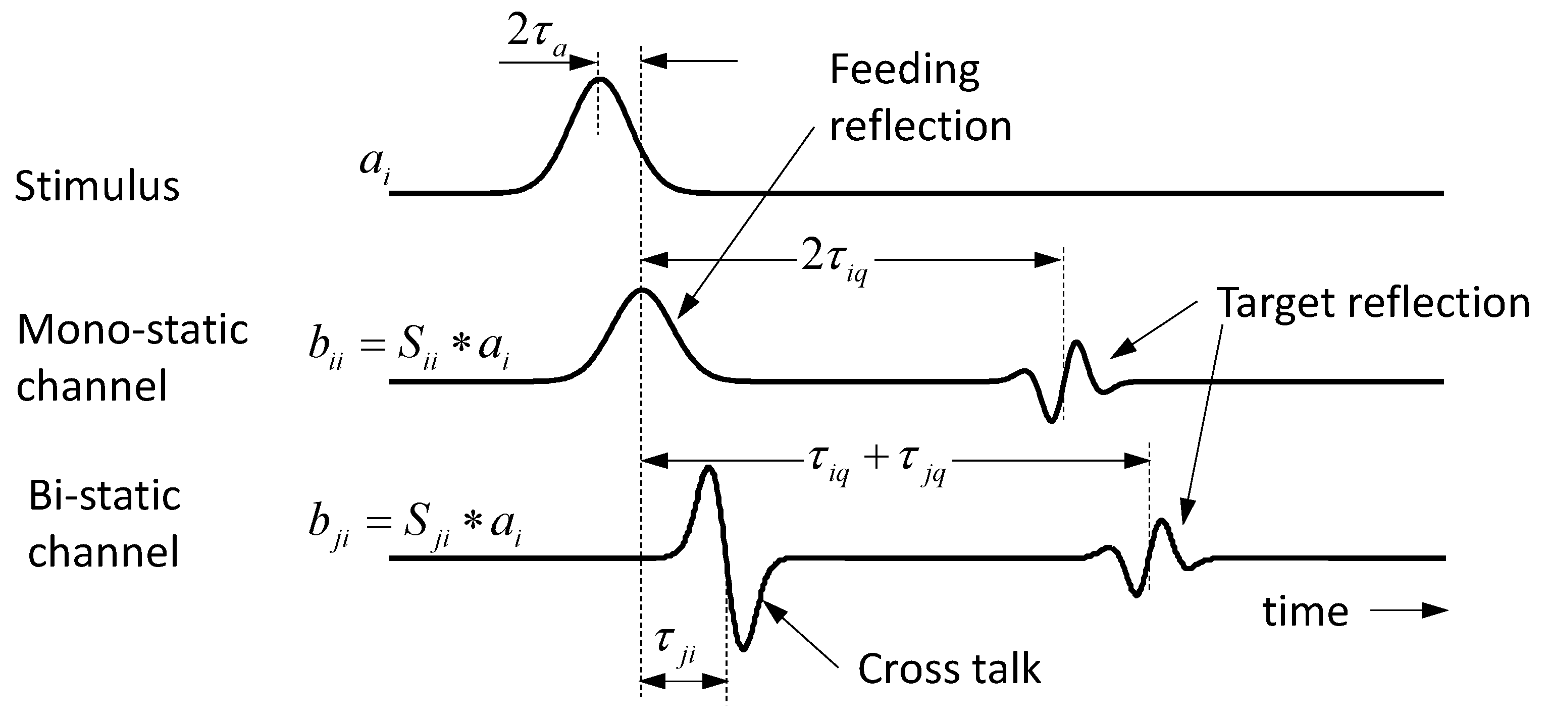
2. Signal Model for Small Time-Variant Scattering Objects
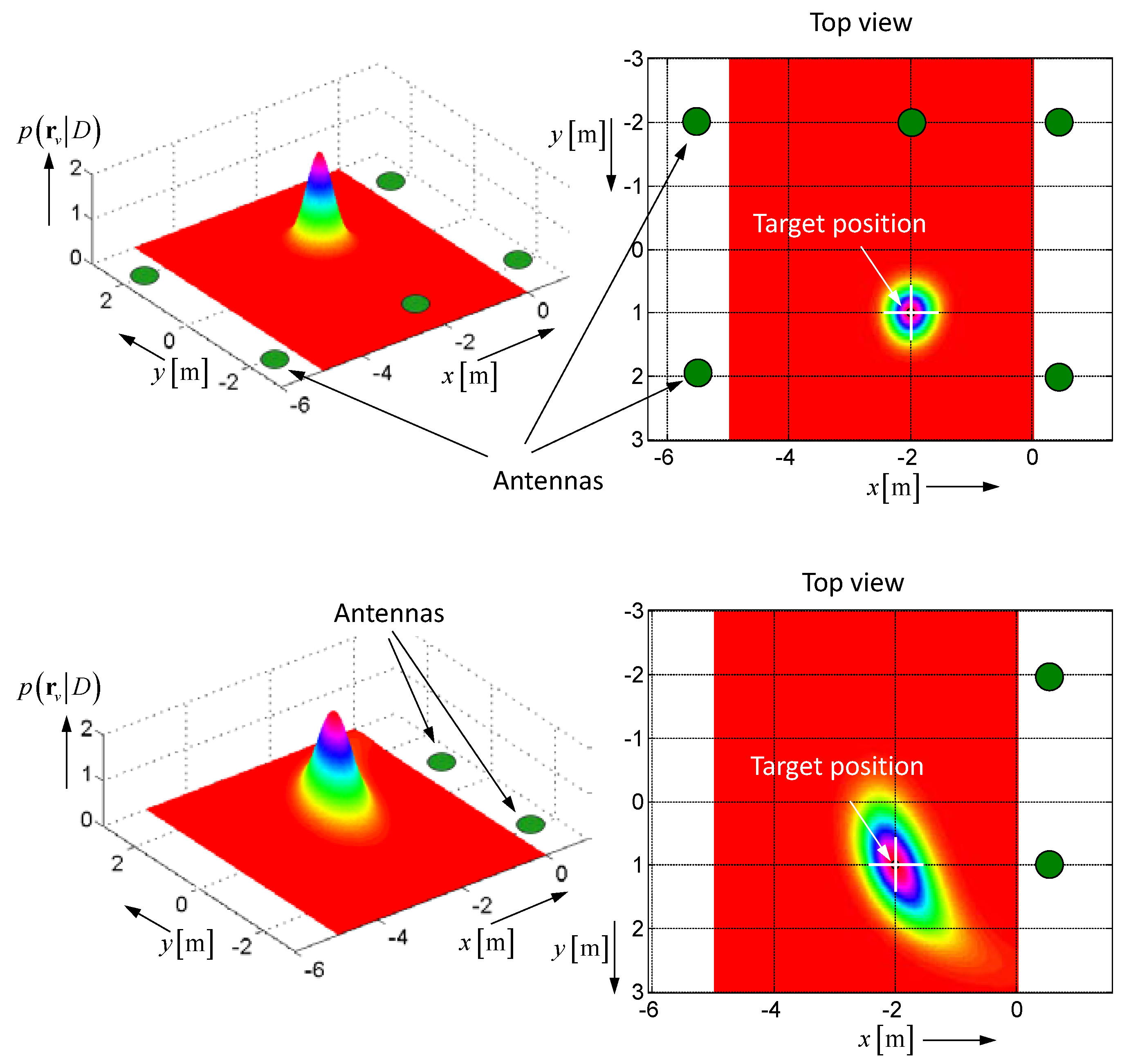
2.1. Invariant Object in Free Space and Its Localization
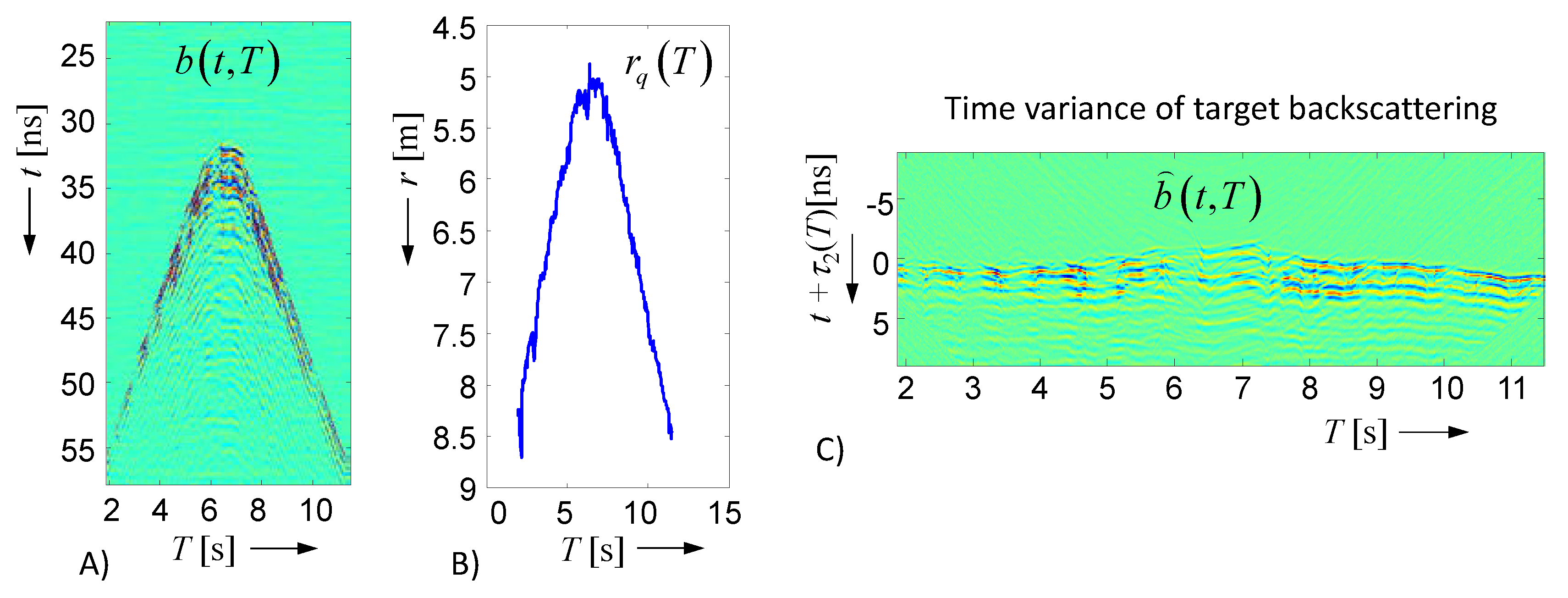
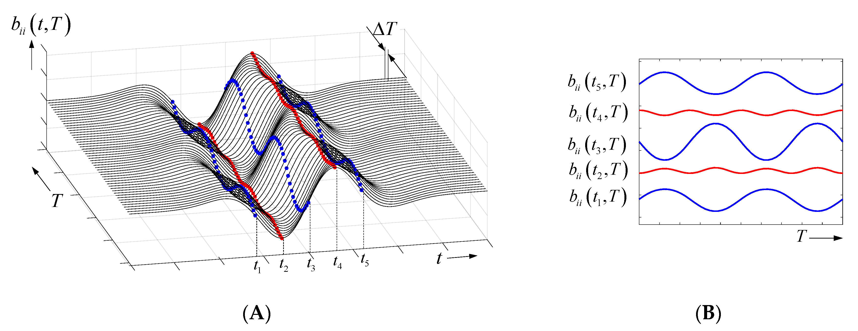
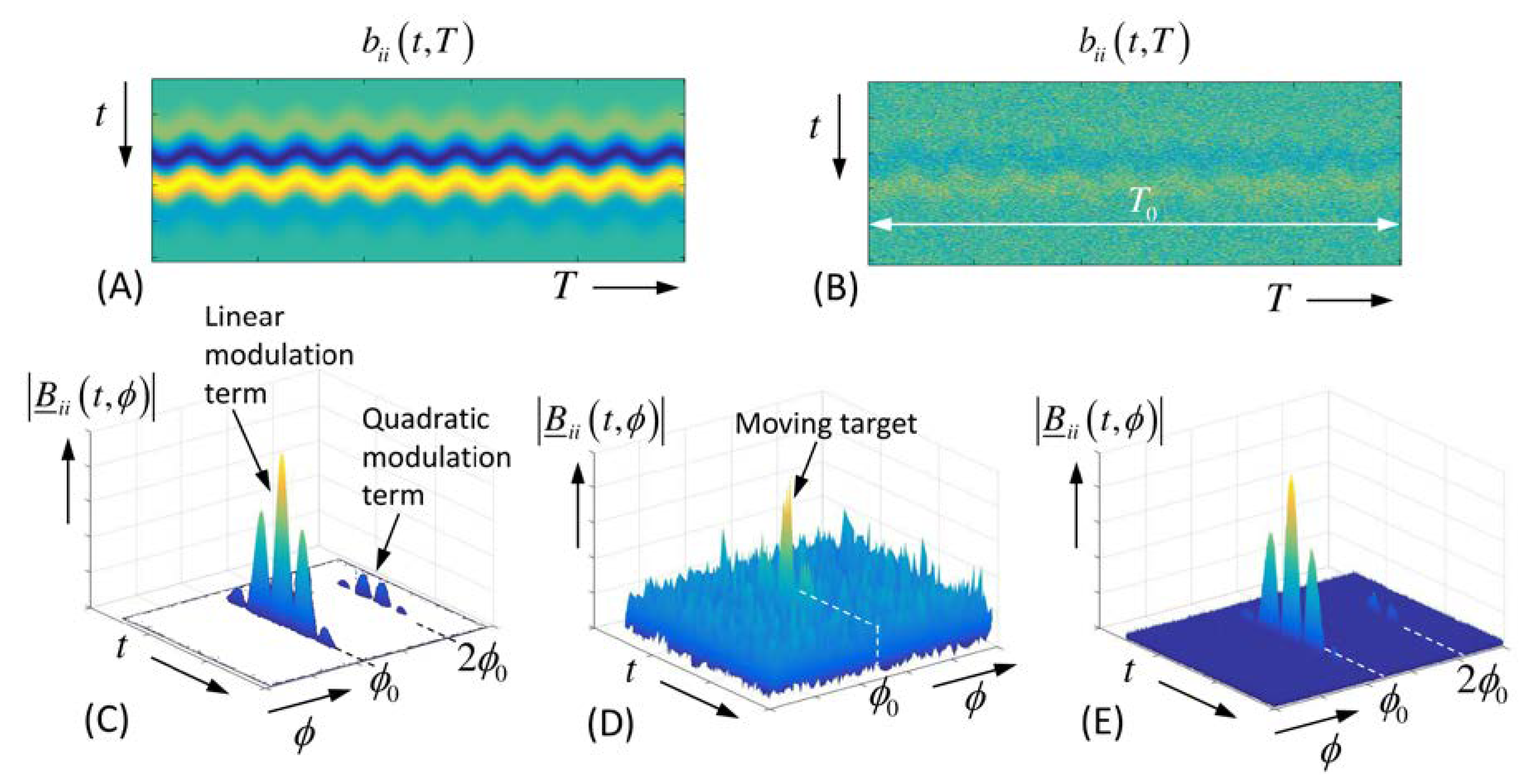
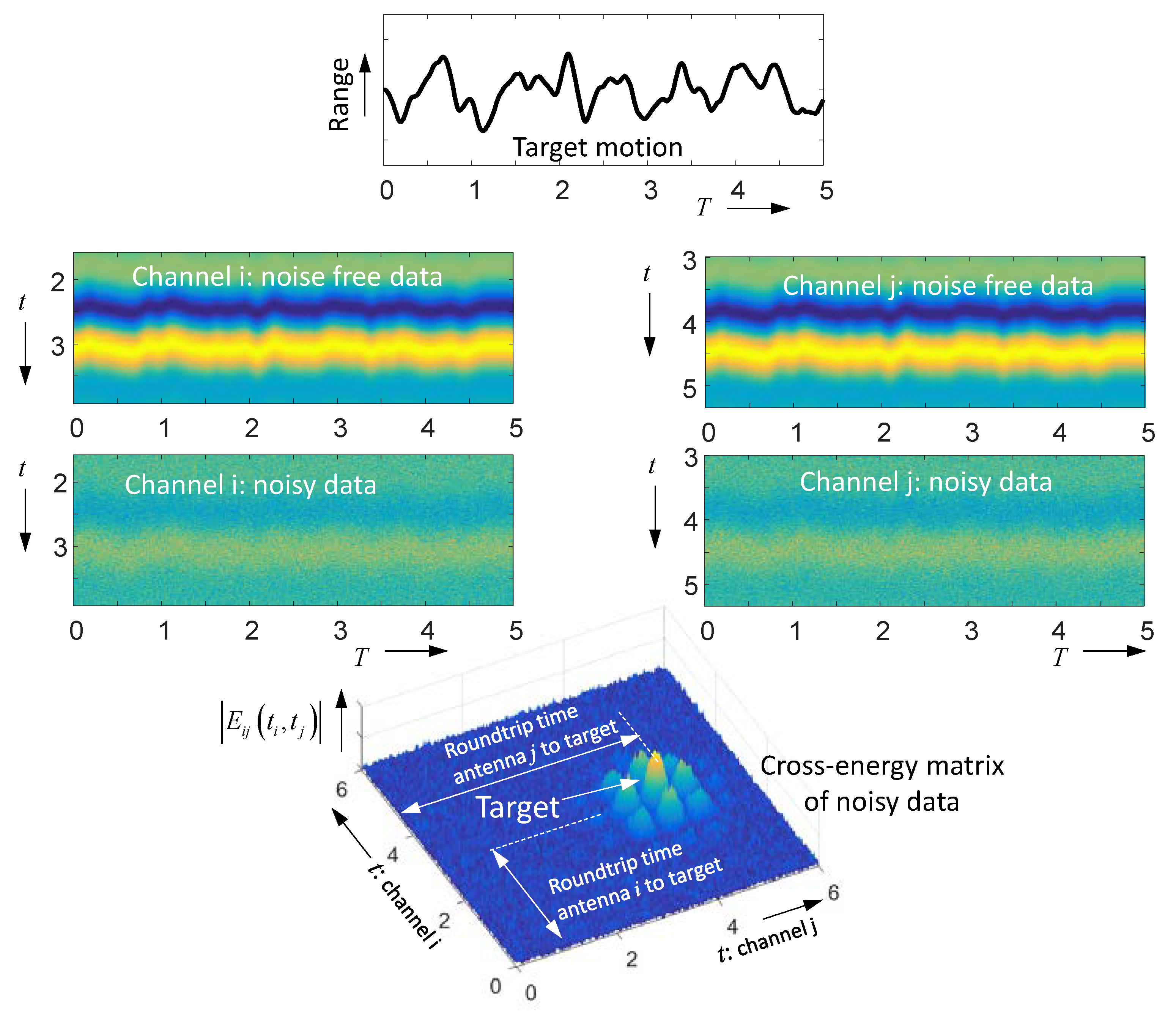
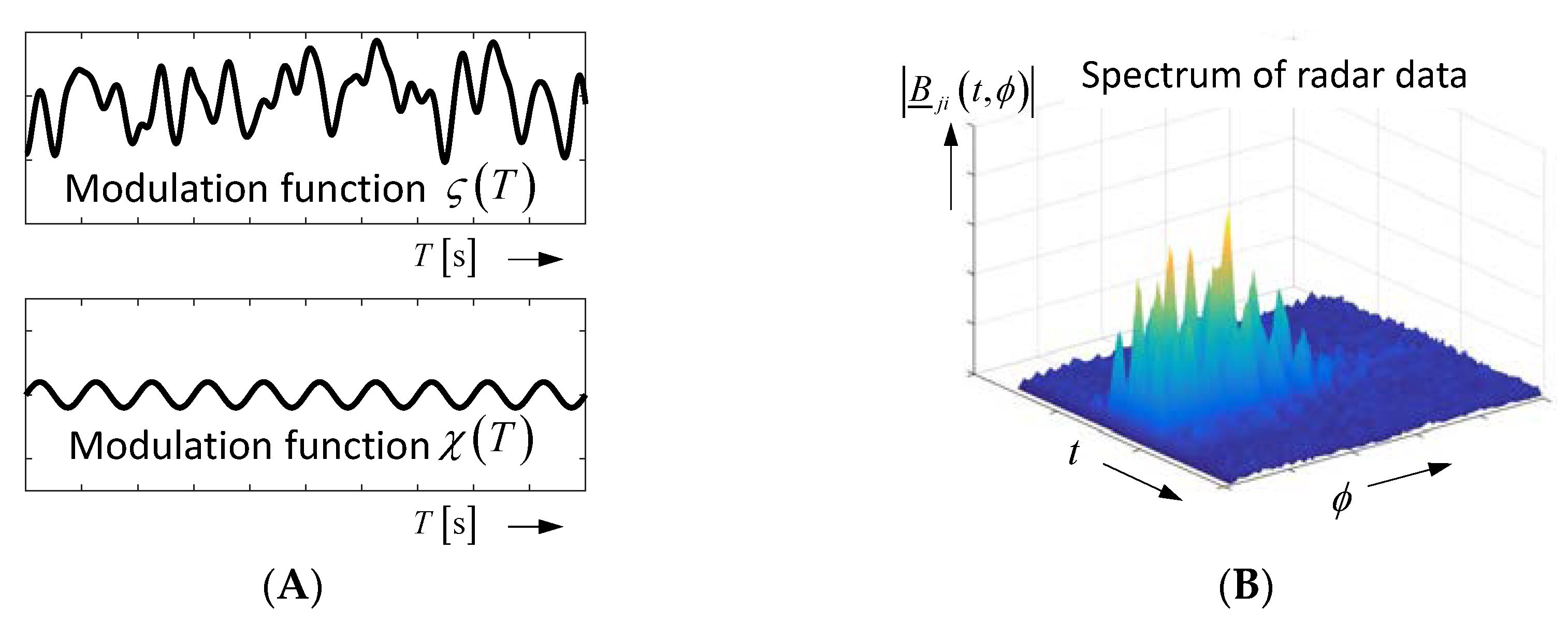
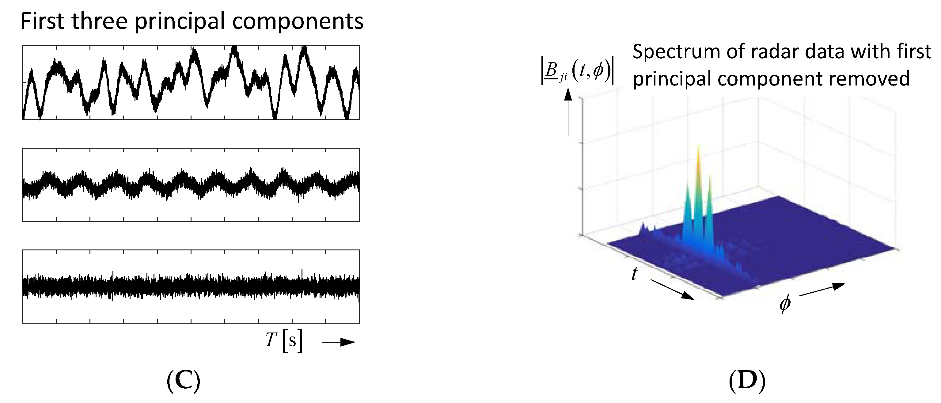
2.2. Time-Variant Objects and Their Emphasis from Noise
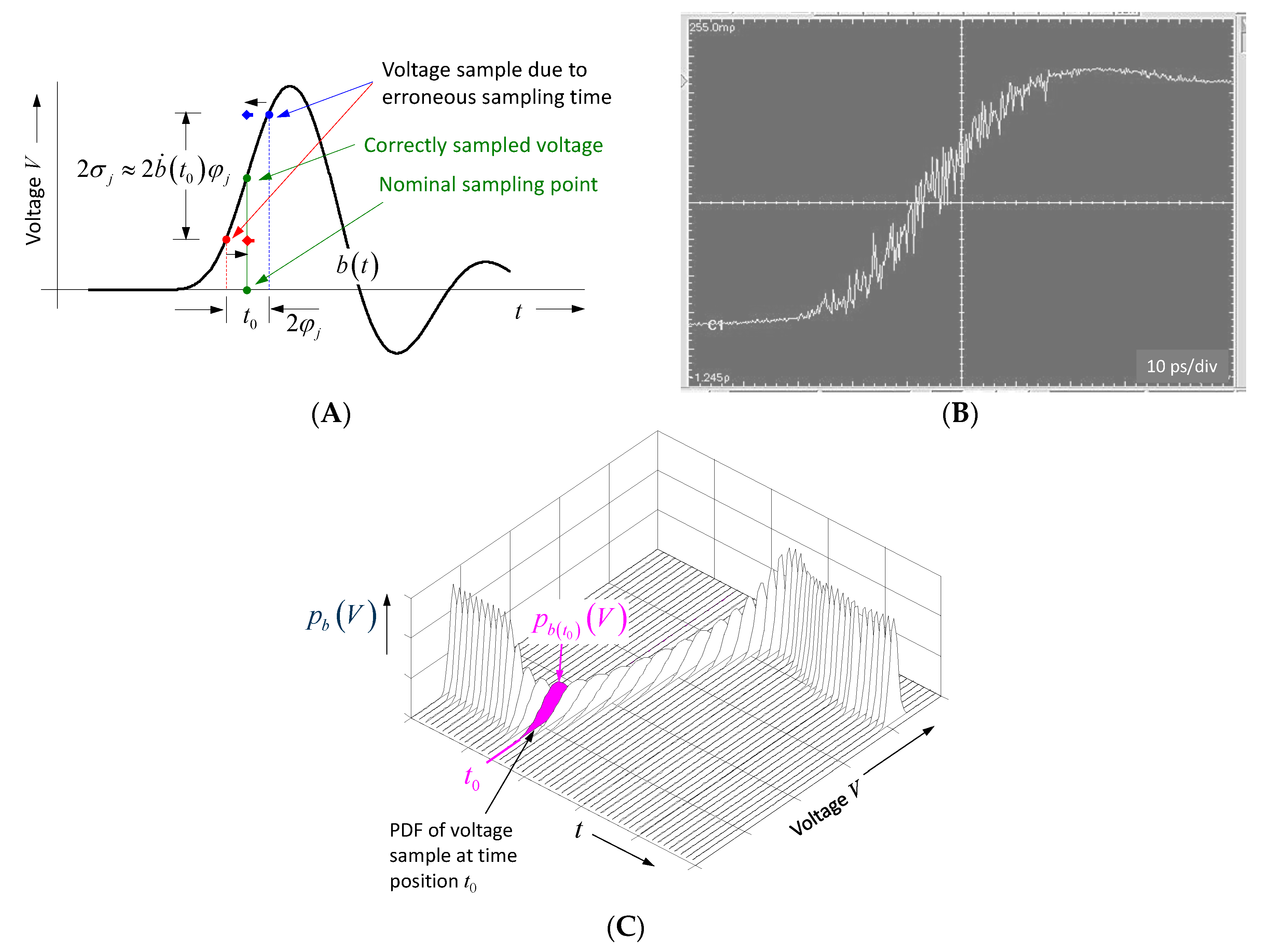
- the largest modulation is provided by the sample located at the steepest part of the received signal;
- the modulations at rising and falling edges are inverted; and
- the modulation at the signal peaks has double frequency (due to the squaring) and is quite weak.
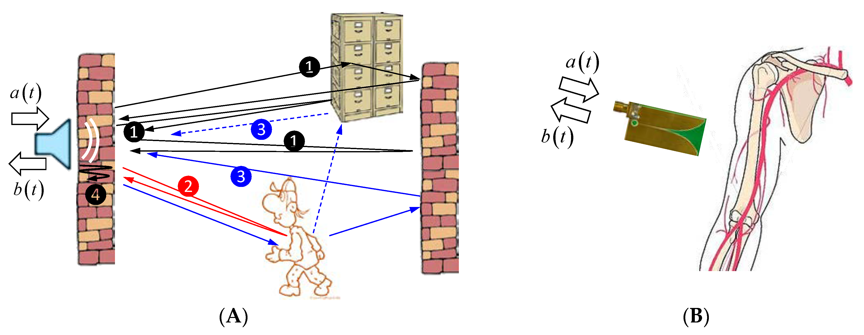
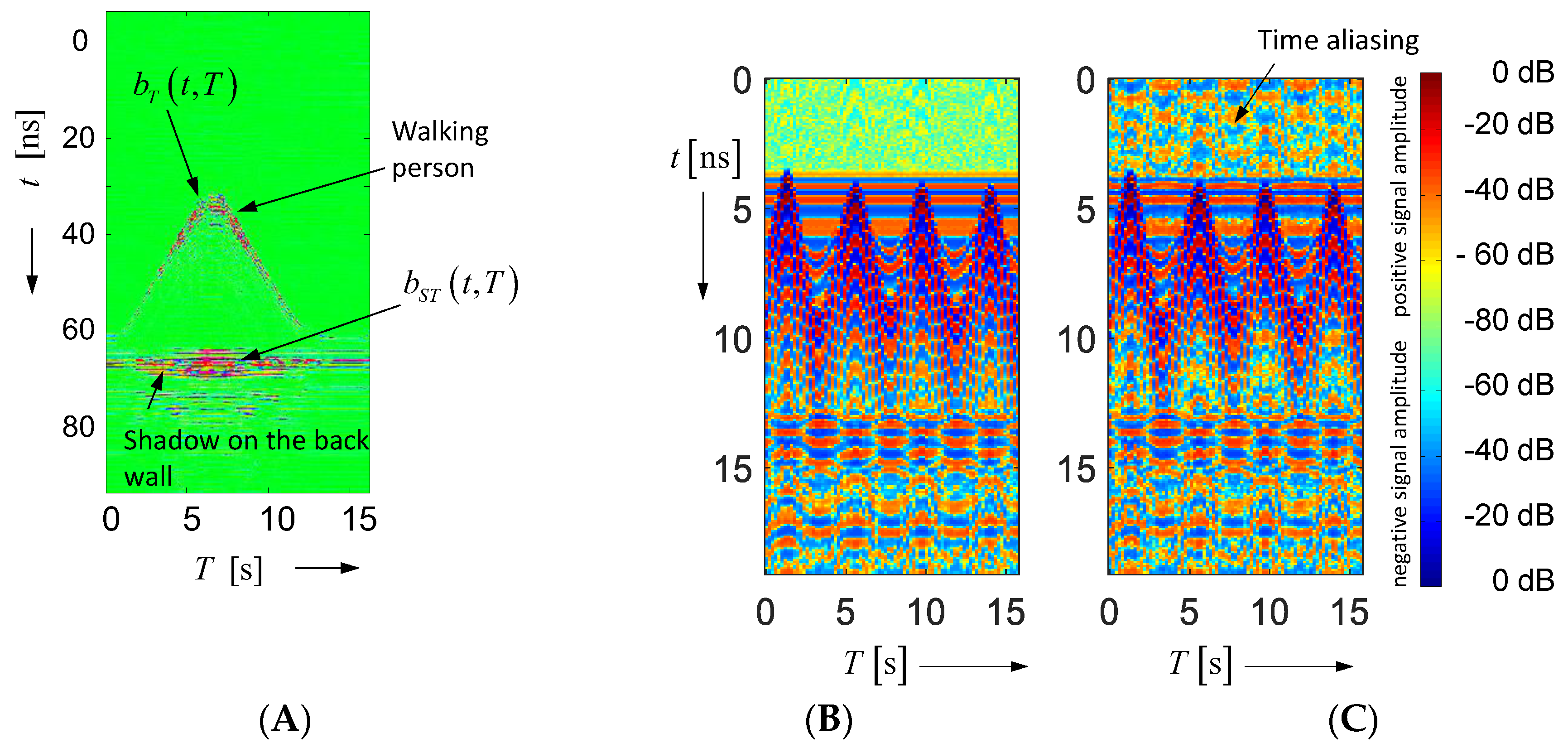
2.3. Time-Variant Objects in Multi-Path Environment
3. Device Requirements for Differential Imaging
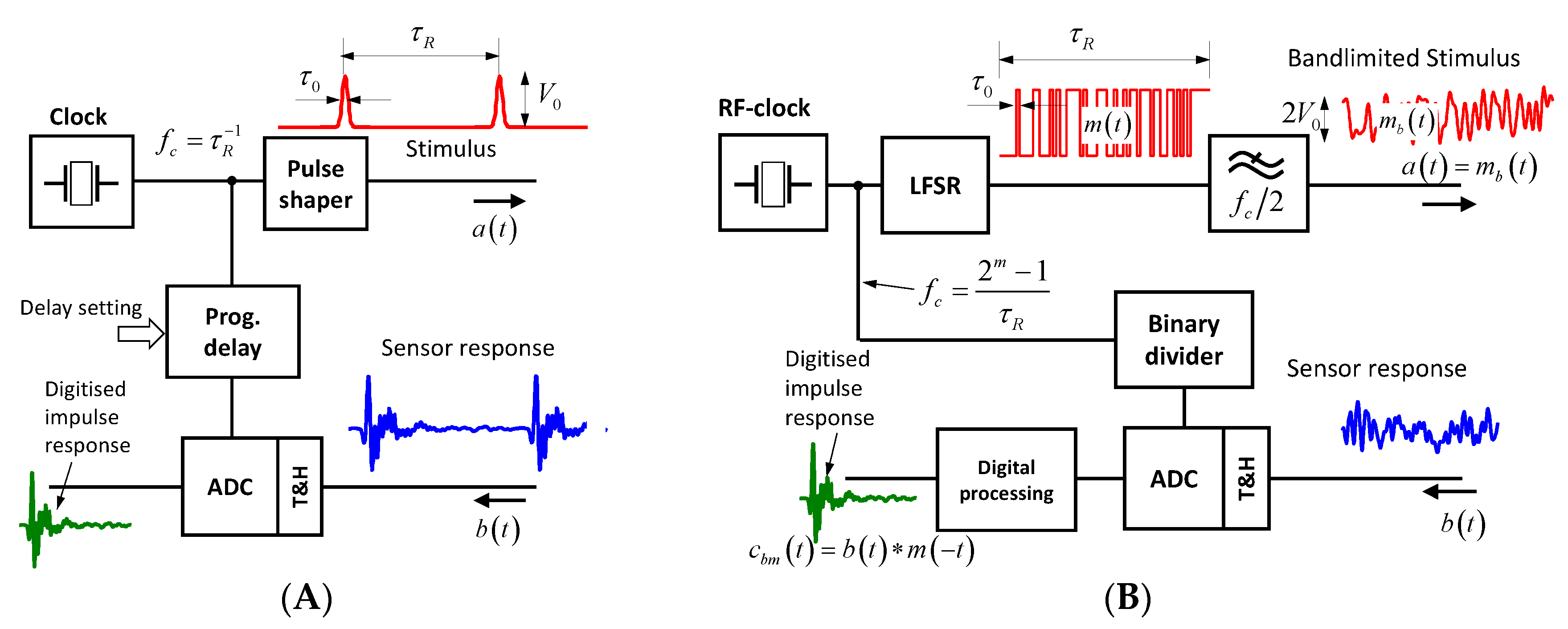
3.1. Pulse and M-Sequence Radar
3.2. Bandwidth, Measurement Rate, and Antenna Array
3.3. Unambiguity Range and Data Throughput
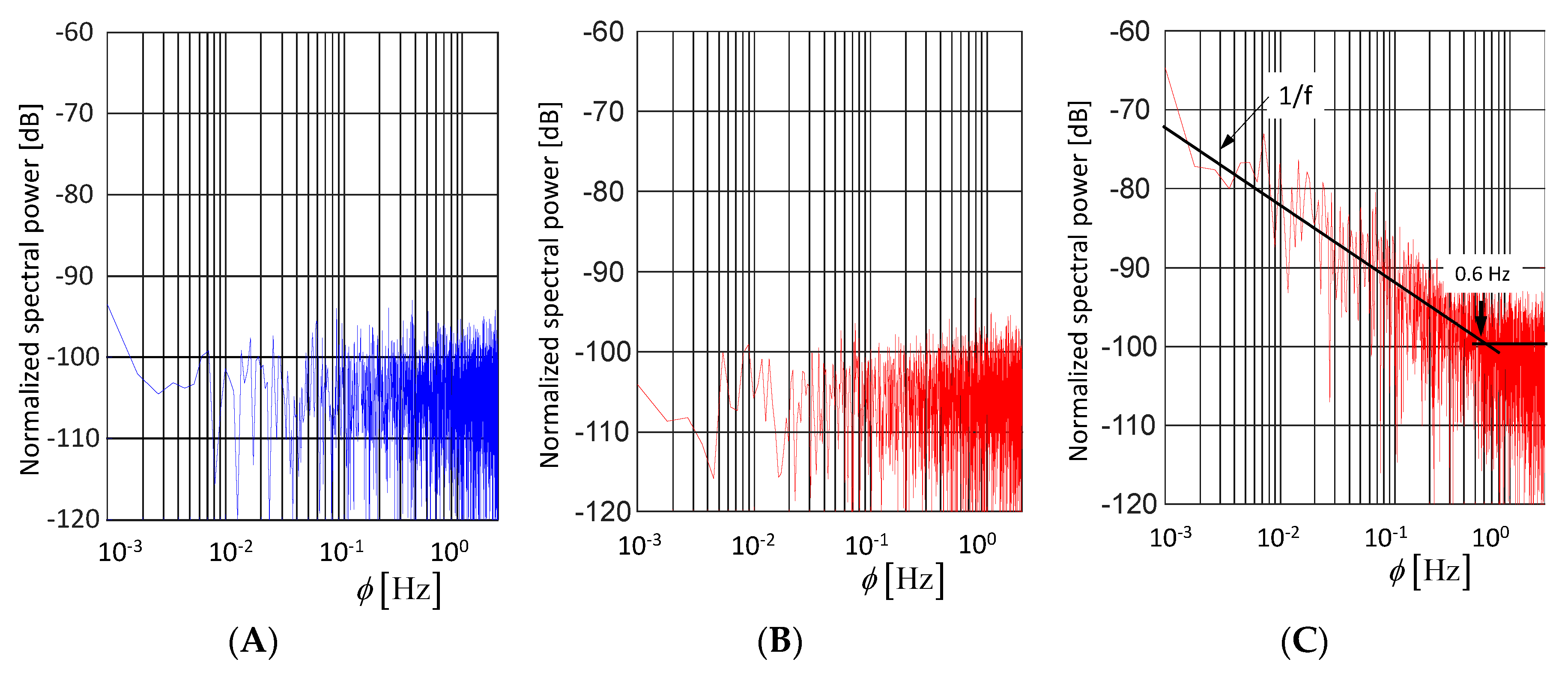
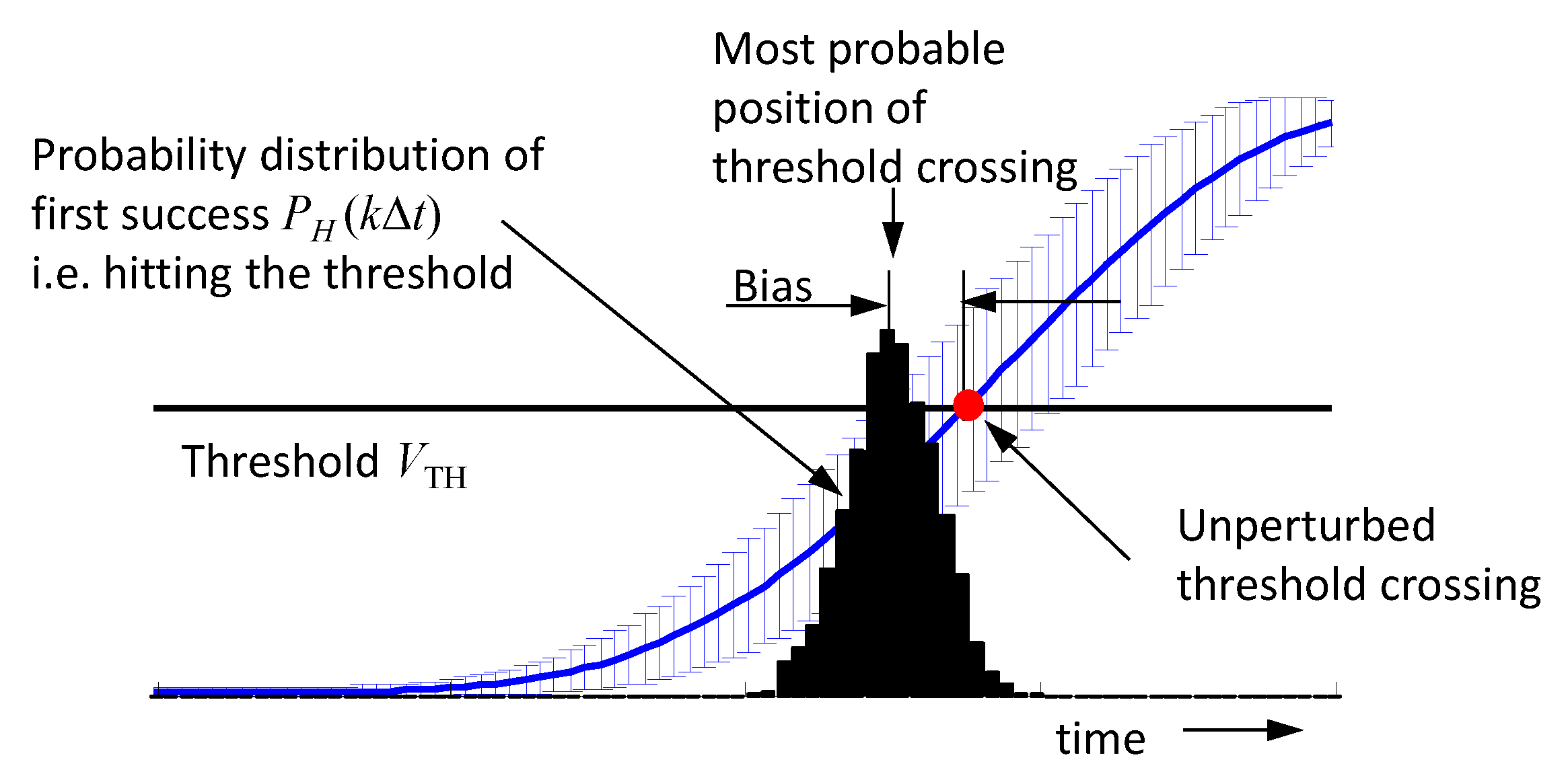
3.4. Random Effects
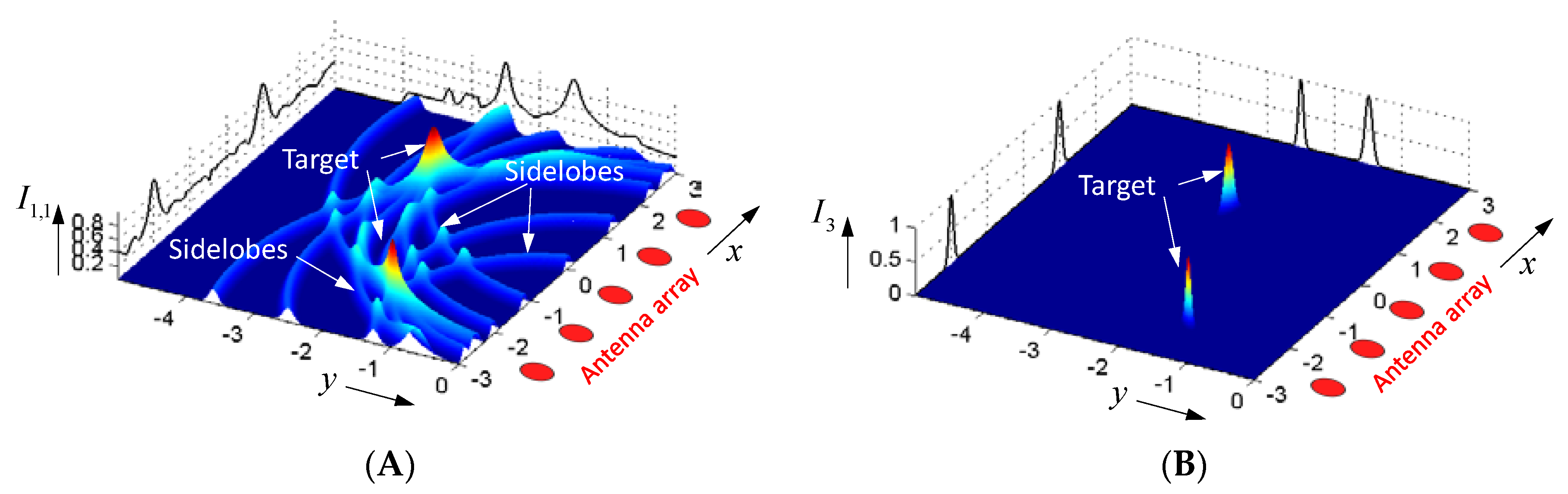
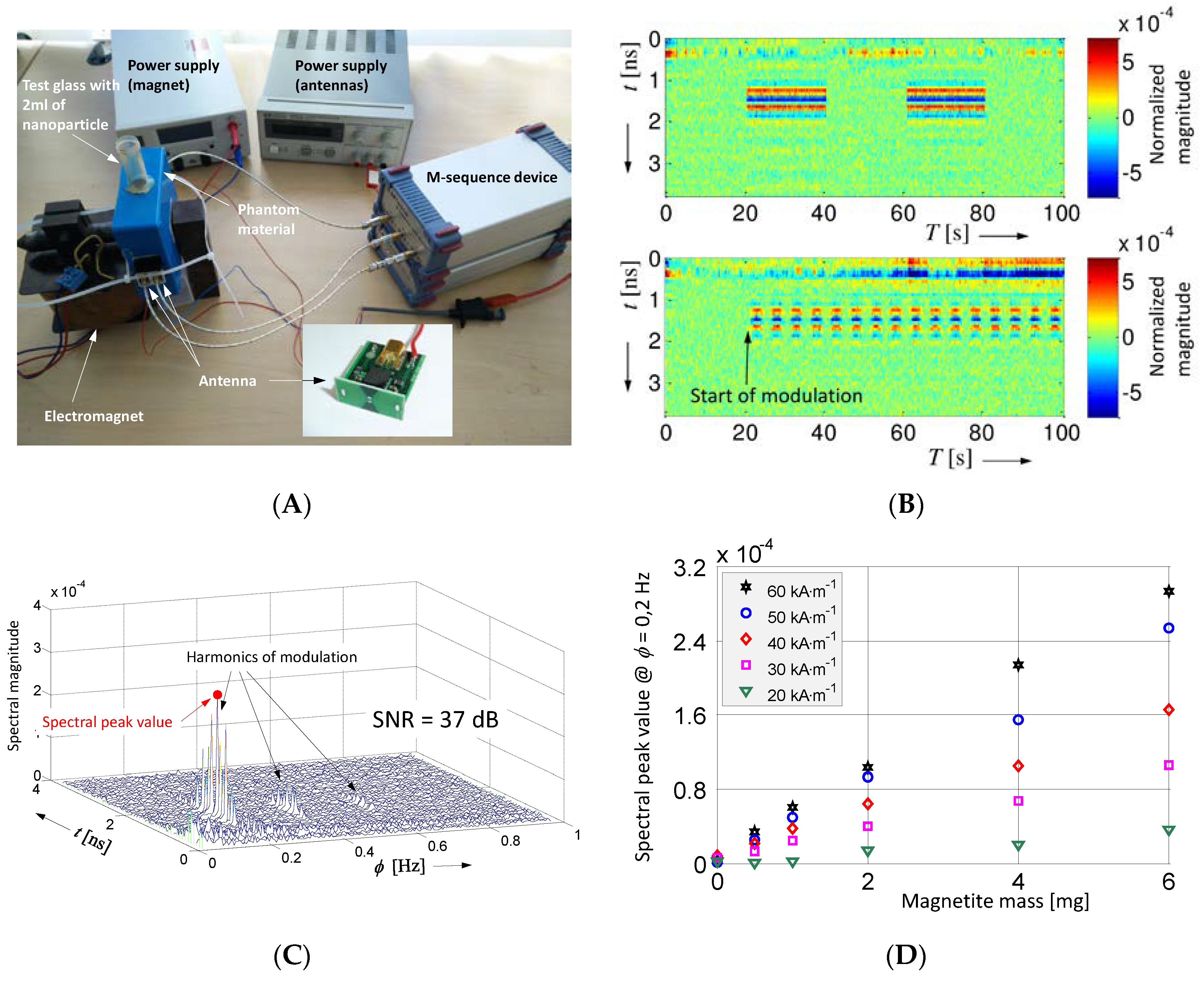
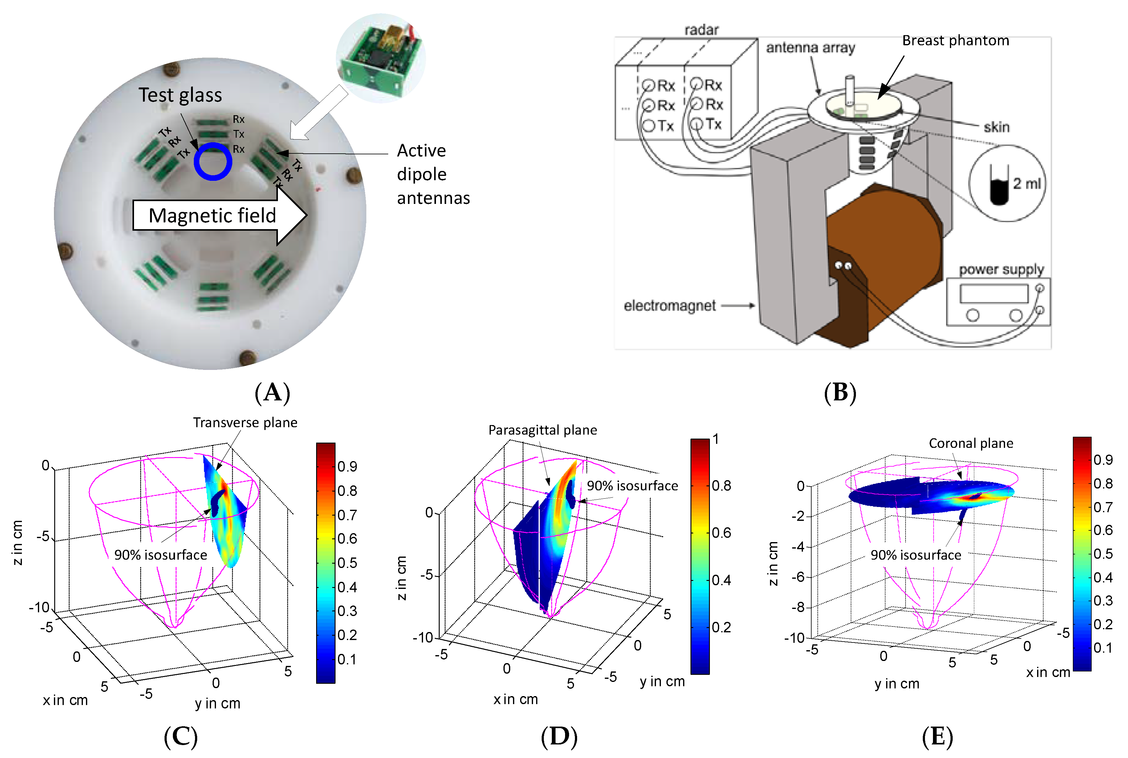
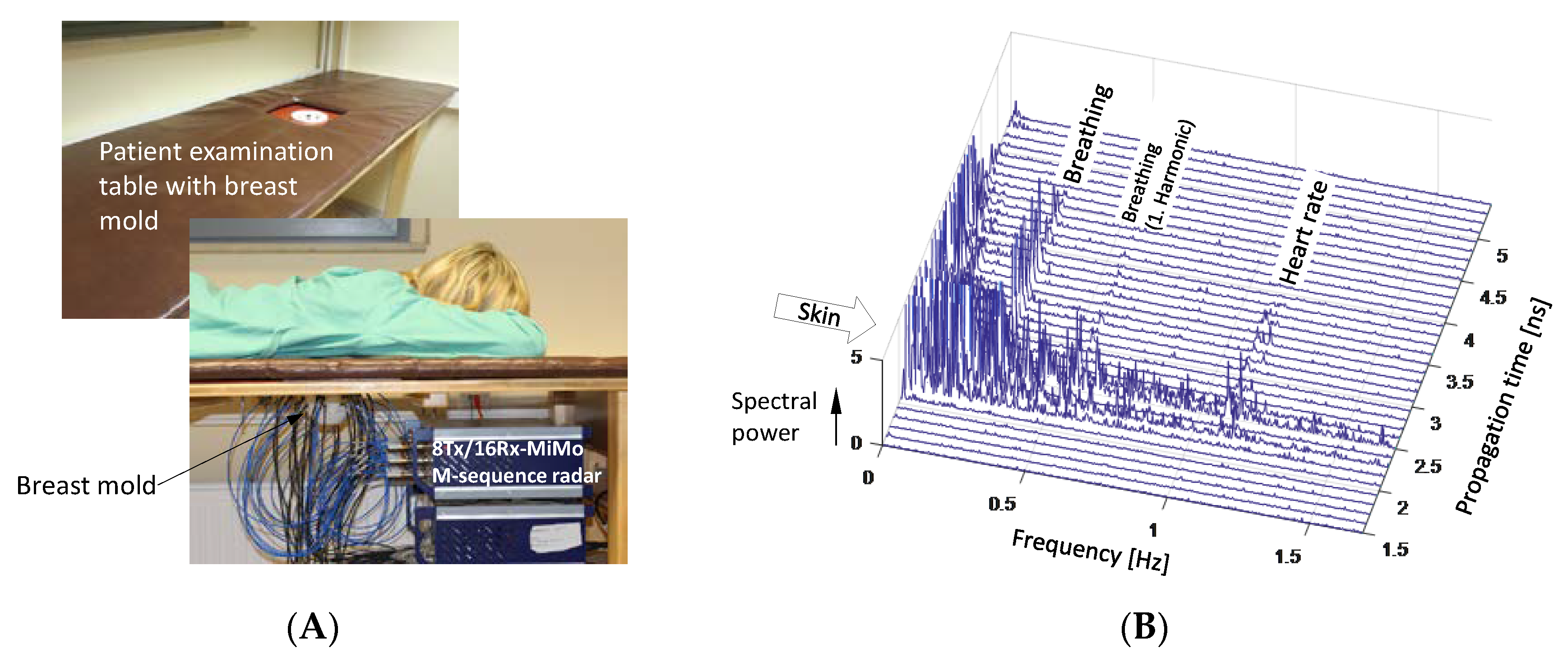
4. Demonstration Examples
5. Conclusions
Author Contributions
Funding
Conflicts of Interest
References
- Sachs, J. Handbook of Ultra-Wideband Short-Range Sensing-Theory, Sensors, Applications; Wiley-VCH: Berlin, Germany, 2012; p. 840. [Google Scholar]
- Nikolova, N.K. Introduction to Microwave Imaging; Cambridge University Press: Cambridge, UK, 2017. [Google Scholar]
- Palmeri, R.; Bevacqua, M.T.; Donato, L.D.; Crocco, L.; Isernia, T. Microwave imaging of non-weak targets in stratified media via virtual experiments and compressive sensing. In Proceedings of the 11th European Conference on Antennas and Propagation (EUCAP), Paris, France, 19–24 March 2017; pp. 1711–1715. [Google Scholar]
- Meo, S.D.; Espín-López, P.F.; Martellosio, A.; Pasian, M.; Matrone, G.; Bozzi, M.; Magenes, G.; Mazzanti, A.; Perregrini, L.; Svelto, F.; et al. On the feasibility of breast cancer imaging systems at millimeter-waves frequencies. IEEE Trans. Microw. Theory Tech. 2017, 65, 1795–1806. [Google Scholar] [CrossRef]
- Zhuge, X.; Yarovoy, A.G. Study on two-dimensional sparse mimo uwb arrays for high resolution near-field imaging. IEEE Trans. Antennas Propag. 2012, 60, 4173–4182. [Google Scholar] [CrossRef]
- Lee, D.; Velander, J.; Nowinski, D.; Augustine, R. A preliminary research on skull healing utilizing short pulsed radar technique on layered cranial surgery phantom models. Prog. Electromagn. Res. 2018, 84, 1–9. [Google Scholar] [CrossRef]
- Scapaticci, R.; Bucci, O.M.; Catapano, I.; Crocco, L. Differential microwave imaging for brain stroke followup. Int. J. Antennas Propag. 2014, 2014. [Google Scholar] [CrossRef]
- Haynes, M.; Stang, J.; Moghaddam, M. Real-time microwave imaging of differential temperature for thermal therapy monitoring. IEEE Trans. Biomed. Eng. 2014, 61, 1787–1797. [Google Scholar] [CrossRef] [PubMed]
- Scapaticci, R.; Bellizzi, G.G.; Cavagnaro, M.; Lopresto, V.; Crocco, L. Exploiting microwave imaging methods for real-time monitoring of thermal ablation. Int. J. Antennas Propag. 2017, 2017. [Google Scholar] [CrossRef]
- Abbosh, A.M.; Mohammed, B.; Bialkowski, K. Differential microwave imaging of breast pair for tumor detection. In Proceedings of the IEEE MTT-S 2015 International Microwave Workshop Series on RF and Wireless Technologies for Biomedical and Healthcare Applications (IMWS-BIO), Taipei, Taiwan, 21–23 September 2015; pp. 63–64. [Google Scholar]
- Margrave, G.F. Numerical Methods of Exploration Seismology with Algorithms in MATLAB. 2001. Available online: https://www.crewes.org/ResearchLinks/FreeSoftware/NumMeth.pdf (accessed on 2 June 2018).
- Savelyev, T.G.; Van Kempen, L.; Sahli, H. Deconvolution techniques. In Ground Penetrating Radar, 2nd ed.; Daniels, D., Ed.; Institution of Electrical Engineers: London, UK, 2004. [Google Scholar]
- Bond, E.J.; Xu, L.; Hagness, S.C.; Van Veen, B.D. Microwave imaging via space-time beamforming for early detection of breast cancer. In Proceedings of the 2002 IEEE International Conference on Acoustics, Speech, and Signal Processing, Orlando, FL, USA, 13–17 May 2002; pp. III-2909–III-2912. [Google Scholar]
- Jian, L.; Stoica, P.; Zhisong, W. On robust capon beamforming and diagonal loading. IEEE Trans. Signal Process. 2003, 51, 1702–1715. [Google Scholar] [CrossRef]
- Lorenz, R.G.; Boyd, S.P. Robust minimum variance beamforming. IEEE Trans. Signal Process. 2005, 53, 1684–1696. [Google Scholar] [CrossRef]
- Hooi Been, L.; Nguyen Thi Tuyet, N.; Er-Ping, L.; Nguyen Duc, T. Confocal microwave imaging for breast cancer detection: Delay-multiply-and-sum image reconstruction algorithm. IEEE Trans. Biomed. Eng. 2008, 55, 1697–1704. [Google Scholar] [CrossRef]
- Zetik, R.; Sachs, J.; Thoma, R. Modified cross-correlation back projection for uwb imaging: Numerical examples. In Proceedings of the IEEE International Conference on Ultra-Wideband (ICUWB), Zurich, Switzerland, 5–8 September 2005. [Google Scholar]
- Matrone, G.; Savoia, A.S.; Caliano, G.; Magenes, G. The delay multiply and sum beamforming algorithm in ultrasound b-mode medical imaging. IEEE Trans. Med. Imaging 2015, 34, 940–949. [Google Scholar] [CrossRef] [PubMed]
- Senglee, F.; Kashyap, S. Cross-correlated back projection for uwb radar imaging. In Proceedings of the Antennas and Propagation Society International Symposium, Monterey, CA, USA, 20–25 June 2004. [Google Scholar]
- Zhou, L.; Huang, C.; Su, Y. A fast back-projection algorithm based on cross correlation for GPR imaging. IEEE Geosci. Remote Sens. Lett. 2012, 9, 228–232. [Google Scholar] [CrossRef]
- Sachs, J.; Herrmann, R.; Kmec, M. Time and range accuracy of short-range ultra-wideband pseudo-noise radar. Appl. Radio Electron. 2013, 12, 105–113. [Google Scholar]
- Sachs, J. On the range estimation by uwb-radar. In Proceedings of the IEEE International Conference on Ultra-Wideband (ICUWB), Paris, France, 1–3 September 2014. [Google Scholar]
- Kerbrat, E.; Prada, C.; Cassereau, D.; Ing, R.K.; Fink, M. Detection and imaging in complex media with the D.O.R.T. Method. In Proceedings of the IEEE Ultrasonics Symposium, San Juan, Puerto Rico, USA, 22–25 October 2000. [Google Scholar]
- Devaney, A.J. Time reversal imaging of obscured targets from multistatic data. IEEE Trans. Antennas Propag. 2005, 53, 1600–1610. [Google Scholar] [CrossRef]
- Bellomo, L.; Saillard, M.; Pioch, S.; Belkebir, K.; Chaumet, P. An ultrawideband time reversal-based radar for microwave-range imaging in cluttered media. In Proceedings of the 13th International Conference on Ground Penetrating Radar (GPR), Lecce, Italy, 21–25 June 2010. [Google Scholar]
- Kosmas, P.; Laranjeira, S.; Dixon, J.H.; Li, X.; Chen, Y. Time reversal microwave breast imaging for contrast-enhanced tumor classification. In Proceedings of the 2010 Annual International Conference of the IEEE Engineering in Medicine and Biology Society (EMBC), Buenos Aires, Argentina, 31 August–4 September 2010. [Google Scholar]
- Yavuz, M.E.; Teixeira, F.L. Ultrawideband microwave sensing and imaging using time-reversal techniques: A review. Remote Sens. 2009, 1, 466–495. [Google Scholar] [CrossRef]
- Fink, M.; Prada, C. Acoustic time-reversal mirrors. Inverse Probl. 2001, 17, R1–R38. [Google Scholar] [CrossRef]
- Zhen, Z.; Fang, L. Application of wavelet analysis technique in the signal denoising of life sign detection. Phys. Proced. 2012, 24, 2124–2130. [Google Scholar] [CrossRef]
- Li, J.; Liu, L.; Zeng, Z.; Liu, F. Advanced signal processing for vital sign extraction with applications in uwb radar detection of trapped victims in complex environments. IEEE J. Sel. Top. Appl. Earth Obs. Remote Sens. 2014, 7, 783–791. [Google Scholar]
- Nezirovic, A.; Yarovoy, A.G.; Ligthart, L.P. Signal processing for improved detection of trapped victims using uwb radar. IEEE Trans. Geosci. Remote Sens. 2010, 48, 2005–2014. [Google Scholar] [CrossRef]
- Mabrouk, M.; Rajan, S.; Bolic, M.; Batkin, I.; Dajani, H.R.; Groza, V.Z. Detection of human targets behind the wall based on singular value decomposition and skewness variations. In Proceedings of the 2014 IEEE Radar Conference, Cincinnati, OH, USA, 19–23 May 2014; pp. 1466–1470. [Google Scholar]
- Lazaro, A.; Girbau, D.; Villarino, R. Techniques for clutter suppression in the presence of body movements during the detection of respiratory activity through UWB radars. Sensors 2014, 14, 2595–2618. [Google Scholar] [CrossRef] [PubMed]
- Conte, E.; Filippi, A.; Tomasin, S. Ml period estimation with application to vital sign monitoring. IEEE Signal Process. Lett. 2010, 17, 905–908. [Google Scholar] [CrossRef]
- Lv, H.; Qi, F.; Zhang, Y.; Jiao, T.; Liang, F.; Li, Z.; Wang, J. Improved detection of human respiration using data fusion based on a multistatic uwb radar. Remote Sens. 2016, 8, 773. [Google Scholar] [CrossRef]
- Li, W.Z. A new method for non-line-of-sight vital sign monitoring based on developed adaptive line enhancer using low entre frequency uwb radar. Prog. Electromagn. Res. 2013, 133, 535–554. [Google Scholar] [CrossRef]
- Ossberger, G.; Buchegger, T.; Schimback, E.; Stelzer, A.; Weigel, R. Non-invasive respiratory movement detection and monitoring of hidden humans using ultra wideband pulse radar. In Proceedings of the 2004 International Workshop on Joint UWBST & IWUWBS, Kyoto, Japan, 18–21 May 2004. [Google Scholar]
- Zaikov, E. M-sequence radar sensor for search and rescue of survivors beneath collapsed buildings. In Handbook of Ultra-Wideband Short-Range Sensing: Theory, Sensors, Applications; Sachs, J., Ed.; Wiley-VCH: Weinheim, Germany, 2012. [Google Scholar]
- Sachs, J.; Helbig, M.; Herrmann, R.; Kmec, M.; Schilling, K.; Zaikov, E. Remote vital sign detection for rescue, security, and medical care by ultra-wideband pseudo-noise radar. Ad Hoc Netw. 2012, 13, 42–53. [Google Scholar] [CrossRef]
- Blum, A.; Hopcroft, J.; Kannan, R. Foundations of Data Science. 2018. Available online: https://www.cs.cornell.edu/jeh/book.pdf (accessed on 2 June 2018).
- Yunqiang, Y.; Fathy, A.E. Development and implementation of a real-time see-through-wall radar system based on FPGA. IEEE Trans. Geosci. Remote Sens. 2009, 47, 1270–1280. [Google Scholar] [CrossRef]
- Zeng, X.; Monteith, A.; Fhager, A.; Persson, M.; Zirath, H. Noise performance comparison between two different types of time-domain systems for microwave detection. Int. J. Microw. Wirel. Technol. 2017, 9, 535–542. [Google Scholar] [CrossRef]
- Ilmsens. M:Explore. Available online: https://www.uwb-shop.com/products/m-explore/ (accessed on 2 June 2018).
- Elkhouly, E.; Fathy, A.E.; Mahfouz, M.R. Signal detection and noise modeling of a 1-d pulse-based ultra-wideband ranging system and its accuracy assessment. IEEE Trans. Microw. Theory Tech. 2015, 63, 1746–1757. [Google Scholar] [CrossRef]
- Amin, M.G. Through-the-Wall Radar Imaging; CRC Press: Boca Raton, FL, USA, 2011. [Google Scholar]
- Fiser; Helbig, M.; Ley, S.; Sachs, J.; Vrba, J. Feasibility study of temperature change detection in phantom using m-sequence radar. In Proceedings of the 10th European Conference on Antennas and Propagation (EuCAP), Davos, Switzerland, 10–15 April 2016; pp. 1–4. [Google Scholar]
- Sachs, J.; Helbig, M.; Kmec, M.; Herrmann, R.; Schilling, K.; Plattes, S.; Fritsch, H.C. Remote heartbeat capturing of high yield cows by uwb radar. In Proceedings of the International Radar Symposium, Dresden, Germany, 24–26 June 2015. [Google Scholar]
- Sachs, J.; Herrmann, R. M-sequence based ultra-wideband sensor network for vitality monitoring of elders at home. IET Radar Sonar Navig. 2015, 9, 125–137. [Google Scholar] [CrossRef]
- Helbig, M.; Zender, J.; Ley, S.; Sachs, J. Simultaneous electrical and mechanical heart activity registration by means of synchronized ECG and M-sequence UWB sensor. In Proceedings of the 10th European Conference on Antennas and Propagation (EuCAP), Davos, Switzerland, 10–15 April 2016; pp. 1–3. [Google Scholar]
- Kosch, O.; Thiel, F.; Schwarz, U.; di Clemente, F.S.; Hein, M.A.; Seifert, F. UWB cardiovascular monitoring for enhanced magnetic resonance imaging. In Handbook of Ultra-Wideband Short-Range Sensing: Theory, Sensors, Applications; Sachs, J., Ed.; Wiley-VCH: Weinheim, Germany, 2012. [Google Scholar]
- Rovňáková, J.; Kocur, D. Experimental comparison of two UWB radar systems for through-wall tracking application. Acta Electrotech. Inform. 2012, 12, 59–66. [Google Scholar] [CrossRef]
- Helbig, M.; Koch, J.H.; Ley, S.; Herrmann, R.; Kmec, M.; Schilling, K.; Sachs, J. Development and test of a massive MIMO system for fast medical UWB imaging. In Proceedings of the International Conference on Electromagnetics in Advanced Applications (ICEAA), Verona, Italy, 11–15 September 2017; pp. 1331–1334. [Google Scholar]
- Klemm, M.; Leendertz, J.; Gibbins, D.; Craddock, I.J.; Preece, A.; Benjamin, R. Towards contrast enhanced breast imaging using ultra-wideband microwave radar system. In Proceedings of the IEEE Radio and Wireless Symposium (RWS), New Orleans, LA, USA, 10–14 January 2010. [Google Scholar]
- Mashal, A.; Sitharaman, B.; Booske, J.H.; Hagness, S.C. Dielectric characterization of carbon nanotube contrast agents for microwave breast cancer detection. In Proceedings of the IEEE Antennas and Propagation Society International Symposium, Charleston, SC, USA, 1–5 June 2009. [Google Scholar]
- Ley, S.; Helbig, M.; Sachs, J.; Faenger, B.; Hilger, I. Initial volunteer trial based on ultra-wideband pseudo-noise radar. In Proceedings of the IMBioC, Gothenburg, Sweden, 15–17 May 2017. [Google Scholar]
- Bellizzi, G.; Bucci, O.M.; Capozzoli, A. Broadband spectroscopy of the electromagnetic properties of aqueous ferrofluids for biomedical applications. J. Magn. Magn. Mater. 2010, 322, 3004–3013. [Google Scholar] [CrossRef]
- Bellizzi, G.G.; Bellizzi, G.; Bucci, O.M.; Crocco, L.; Helbig, M.; Ley, S.; Sachs, J. Optimization of working conditions for magnetic nanoparticle enhanced ultra-wide band breast cancer detection. In Proceedings of the 10th European Conference on Antennas and Propagation (EuCAP), Davos, Switzerland, 10–15 April 2016; pp. 1–3. [Google Scholar]
- Bellizzi, G.; Bellizzi, G.G.; Bucci, O.M.; Crocco, L.; Helbig, M.; Ley, S.; Sachs, J. Optimization of the working conditions for magnetic nanoparticle-enhanced microwave diagnostics of breast cancer. IEEE Trans. Biomed. Eng. 2018, 65. [Google Scholar] [CrossRef] [PubMed]
- Ley, S.; Helbig, M.; Sachs, J.; Frick, S.; Hilger, I. First trials towards contrast enhanced microwave breast cancer detection by magnetic modulated nanoparticles. In Proceedings of the 9th European Conference on Antennas and Propagation (EuCAP), Lisbon, Portugal, 13–17 April 2015. [Google Scholar]
- Ley, S.; Helbig, M.; Sachs, J. MNP enhanced microwave breast cancer imaging based on ultra-wideband pseudo-noise sensing. In Proceedings of the 11th European Conference on Antennas and Propagation (EUCAP), Paris, France, 19–24 March 2017. [Google Scholar]
- Helbig, M.; Dahlke, K.; Hilger, I.; Kmec, M.; Sachs, J. UWB microwave imaging of heterogeneous breast phantoms. Biomed. Eng. Tech. 2012, 57, 486–489. [Google Scholar] [CrossRef]
- Garrett, J.; Fear, E. A new breast phantom with a durable skin layer for microwave breast imaging. IEEE Trans. Antennas Propag. 2015, 63, 1693–1700. [Google Scholar] [CrossRef]
- Lazebnik, M.; Madsen, E.L.; Frank, G.R.; Hagness, S.C. Tissue-mimicking phantom materials for narrowband and ultrawideband microwave applications. Phys. Med. Biol. 2005, 50, 4245–4258. [Google Scholar] [CrossRef] [PubMed]


© 2018 by the authors. Licensee MDPI, Basel, Switzerland. This article is an open access article distributed under the terms and conditions of the Creative Commons Attribution (CC BY) license (http://creativecommons.org/licenses/by/4.0/).
Share and Cite
Sachs, J.; Ley, S.; Just, T.; Chamaani, S.; Helbig, M. Differential Ultra-Wideband Microwave Imaging: Principle Application Challenges. Sensors 2018, 18, 2136. https://doi.org/10.3390/s18072136
Sachs J, Ley S, Just T, Chamaani S, Helbig M. Differential Ultra-Wideband Microwave Imaging: Principle Application Challenges. Sensors. 2018; 18(7):2136. https://doi.org/10.3390/s18072136
Chicago/Turabian StyleSachs, Jürgen, Sebastian Ley, Thomas Just, Somayyeh Chamaani, and Marko Helbig. 2018. "Differential Ultra-Wideband Microwave Imaging: Principle Application Challenges" Sensors 18, no. 7: 2136. https://doi.org/10.3390/s18072136
APA StyleSachs, J., Ley, S., Just, T., Chamaani, S., & Helbig, M. (2018). Differential Ultra-Wideband Microwave Imaging: Principle Application Challenges. Sensors, 18(7), 2136. https://doi.org/10.3390/s18072136