Estimation of Tri-Axial Walking Ground Reaction Forces of Left and Right Foot from Total Forces in Real-Life Environments


Abstract
1. Introduction
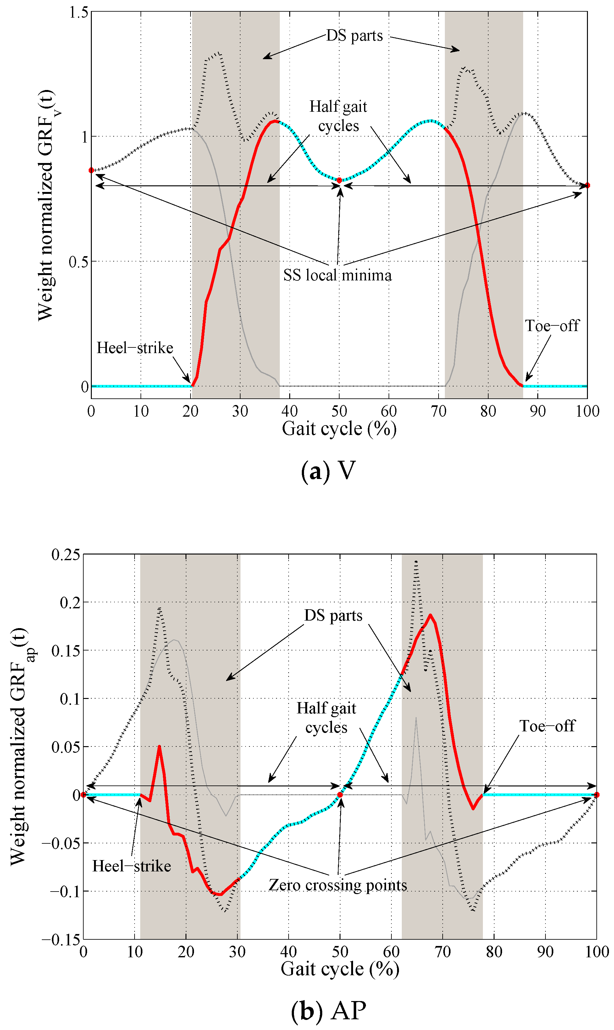
- The ground reaction forces and moments of the trailing foot reduce smoothly to zero during the DS phase.
- The ratios of the ground reactions to their values at contralateral heel strike (i.e., the non-dimensional ground reactions) can be expressed as functions of DS phase duration (termed transition functions).
2. TPM Methodology
2.1. Experimental Data
2.2. TPM Specifications
2.2.1. Identification and Validation Experimental Datasets
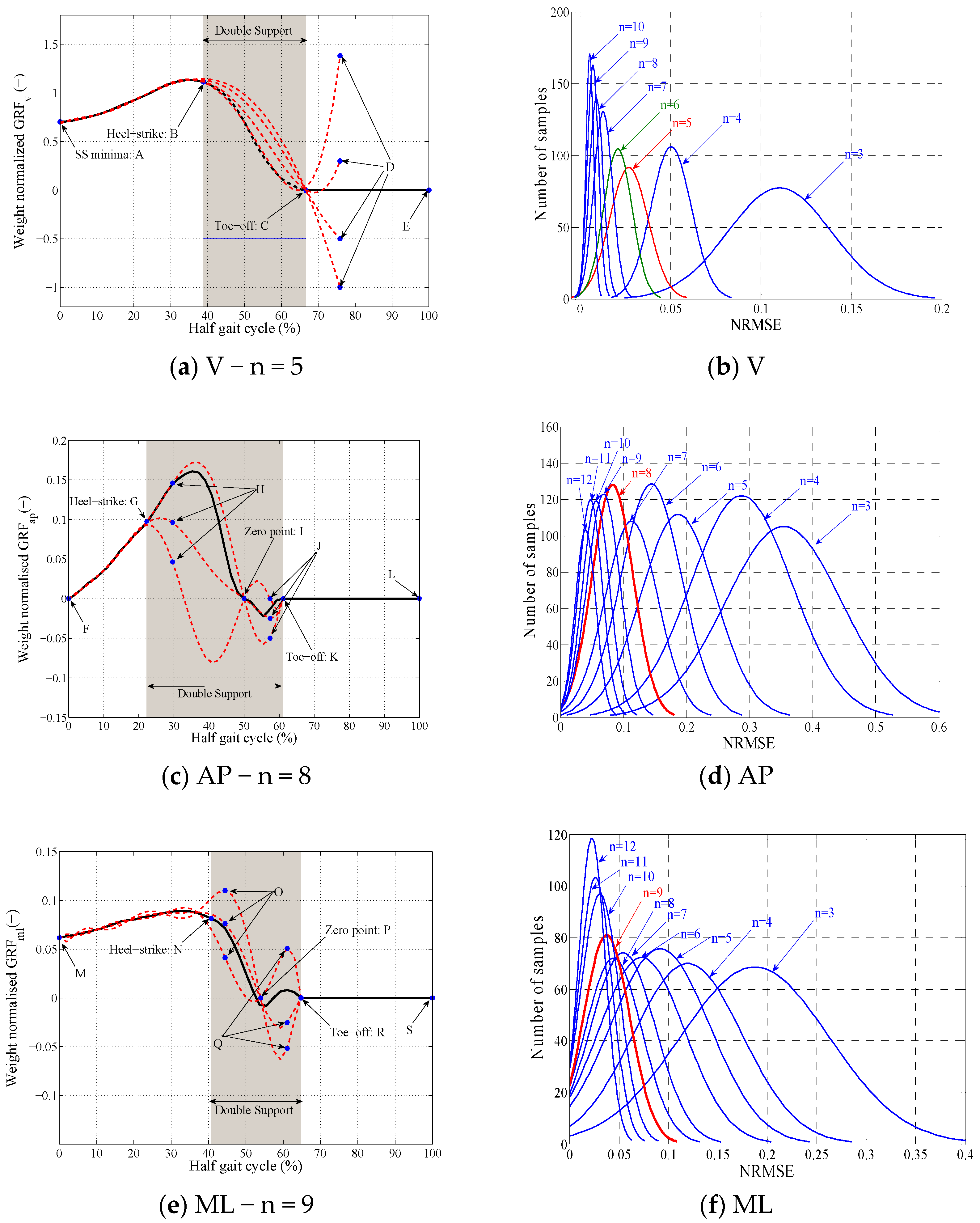
2.2.2. Polynomial Degree Selection
2.2.3. Added Constraints
2.2.4. Optimization Strategy
3. Results
3.1. TPM Procedure
- A.
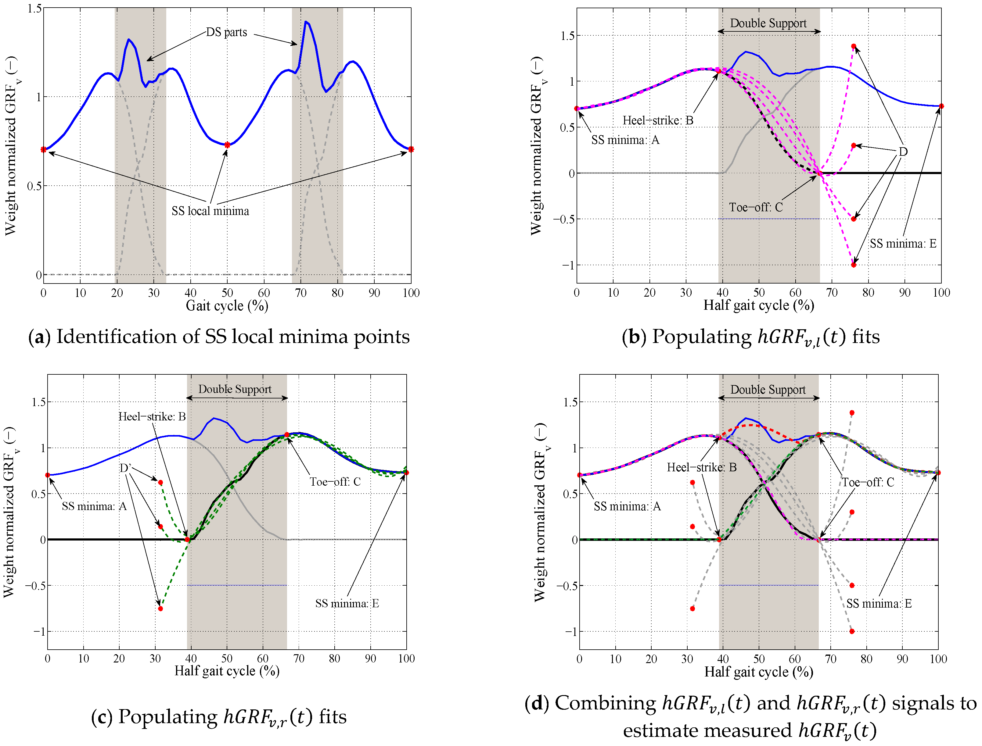
- Vertical direction
- In the first step, the SS local minima points are identified from the total (Figure 5a).
- For each segment of the total signal between two consecutive local minima (total ):
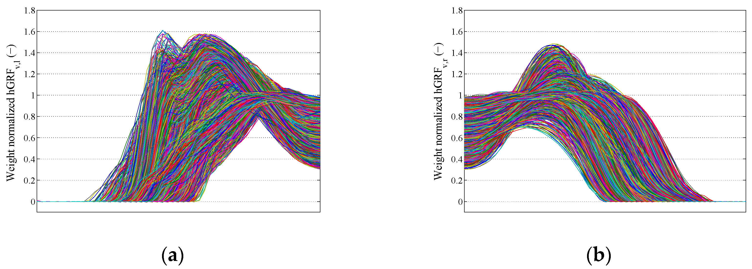
- The total segment is resampled to 100 points (T = 100) and is normalized to the weight of the subject (Figure 5b).
- For each pair of toe-off () and heel-strike () points selected from their initial ranges (27 < 52 and 53 < 85):
- The procedure is repeated for all possible combinations of and selected from their initial ranges (Table 1).
- The pair of left-right polynomial curves that estimated the total with minimum NRMSE is found. These curves are considered accurate estimates of the and signals for the current half gait cycle.
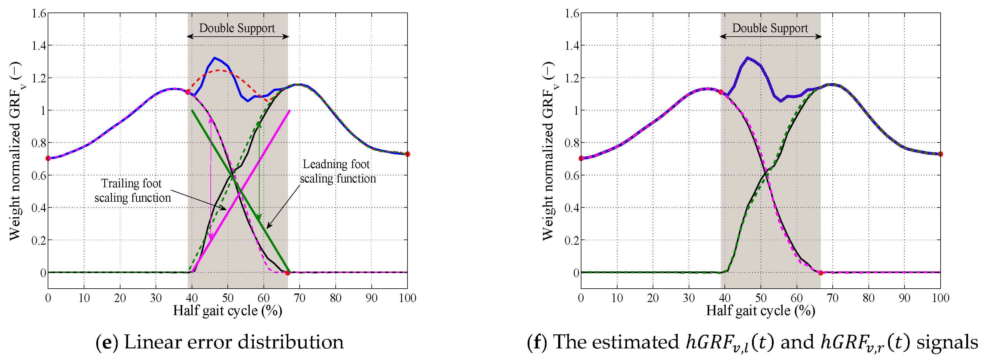
- The estimated and signals (dashed curves in Figure 5f) are multiplied by the weight of the subject and resampled back to the actual length of the measured total signal for the current half gait cycle.
- The next half gait cycle is selected and the estimation procedure described in Step A.II is repeated.
- B.
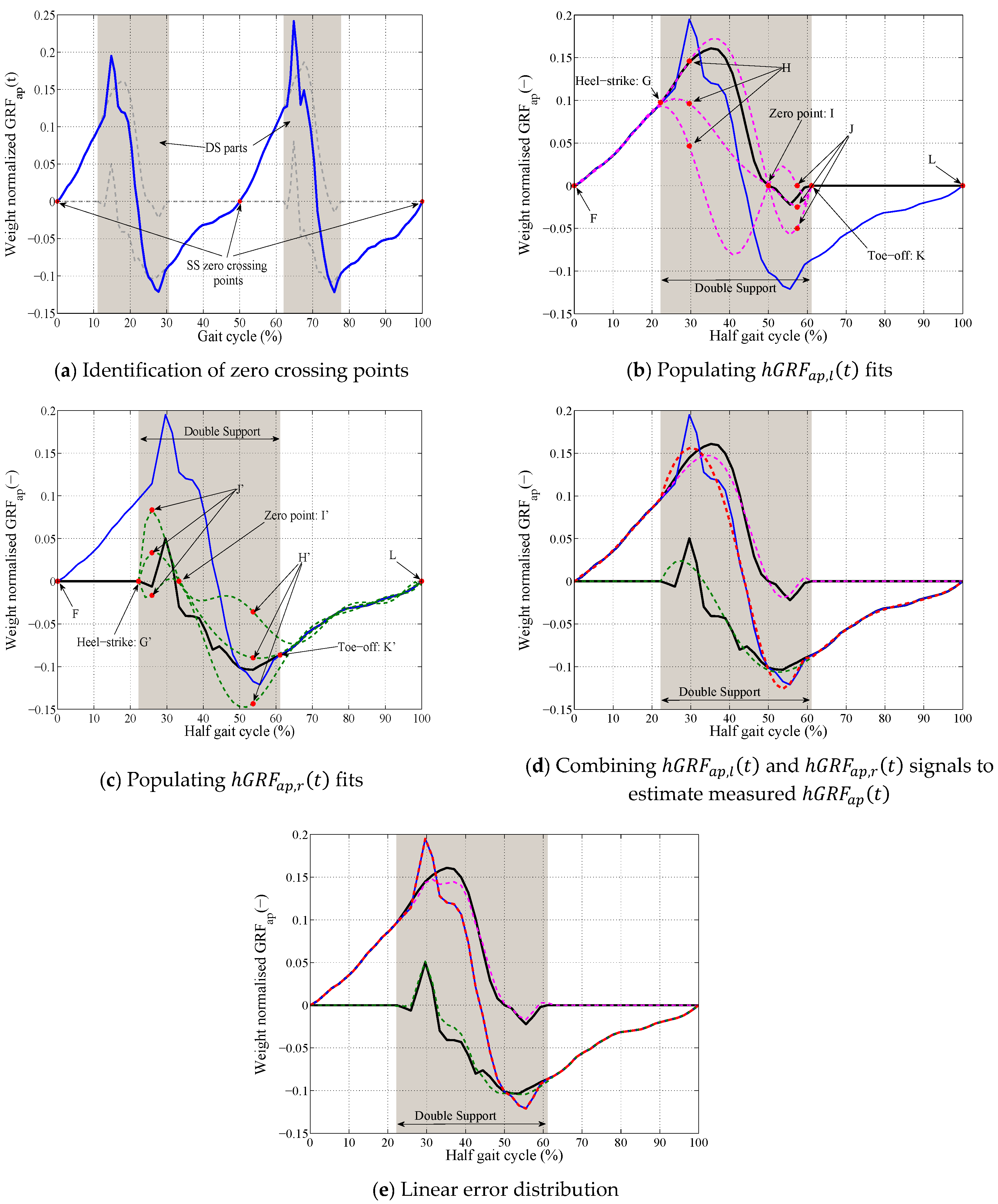
- Anterior-posterior direction
- In the first step, the SS phase zero crossing points are identified from the total (Figure 6a).
- For each segment of the total signal between two consecutive zero crossing points (total :
- The total segment is resampled to 100 points (T = 100) and normalized to the weight of the subject (Figure 6b).
- The timing of the heel-strike () and toe-off () points of this half gait cycle are identified from the previously-estimated and signals corresponding to this half gait cycle.
- The difference between the measured (blue curve in Figure 6d) and estimated total (dashed red curve in Figure 6d) curves during the DS phase , are distributed between the estimated (dashed pink curve in Figure 6d) and (dashed green curve in Figure 6d) signals using Equations (3) and (4) when and (Figure 6e).
- The estimated and signals are multiplied by the weight of the subject and resampled back to the actual length of the measured total signal for the current half gait cycle.
- The next half gait cycle is selected and the estimation procedure described in Step B.II is repeated.
- C.
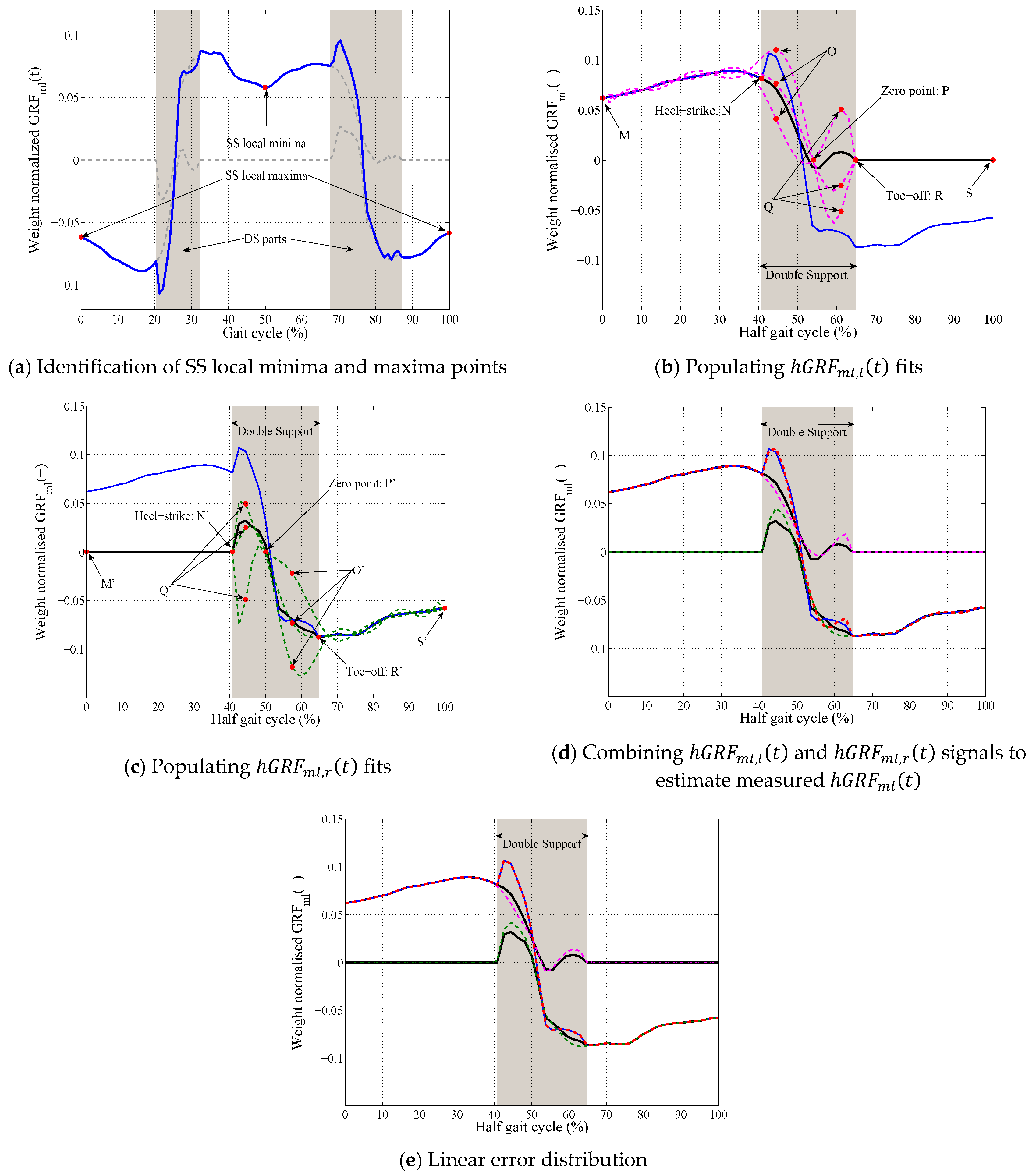
- Medial-lateral direction
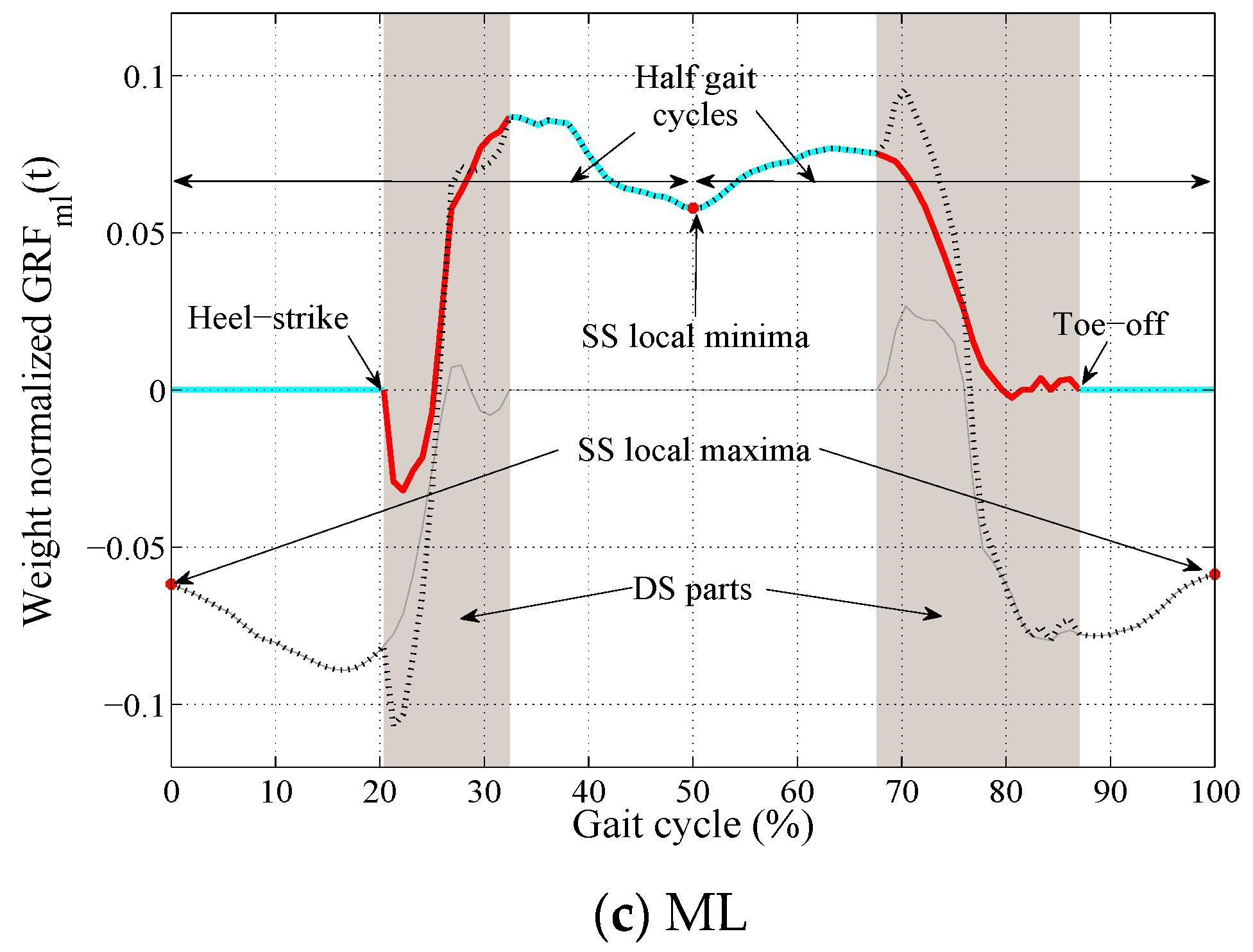
- In the first step, the SS local minima and maxima points are identified from the total (Figure 7a).
- For each segment of the total signal between two consecutive local minima and maxima (total ):
- The total signal is resampled to 100 points (T = 100) and normalized to the weight of the subject (Figure 7b).
- The timing of the heel-strike () and toe-off () points for this half gait cycle are identified from the previously-estimated and signals corresponding to this half gait cycle.
- The difference between the measured (blue curve in Figure 7d) and estimated total (dashed red curve in Figure 7d) curves during the DS phase , are distributed between the estimated (dashed pink curve in Figure 7d) and (dashed green curve in Figure 7d) signals using Equations (3) and (4) when and (Figure 7e).
- The estimated and signals are multiplied by the weight of the subject and resampled back to the actual length of the measured total signal for the current half gait cycle.
- The next half gait cycle is selected and the estimation procedure described in Step C.II is repeated.
3.2. Model Validation
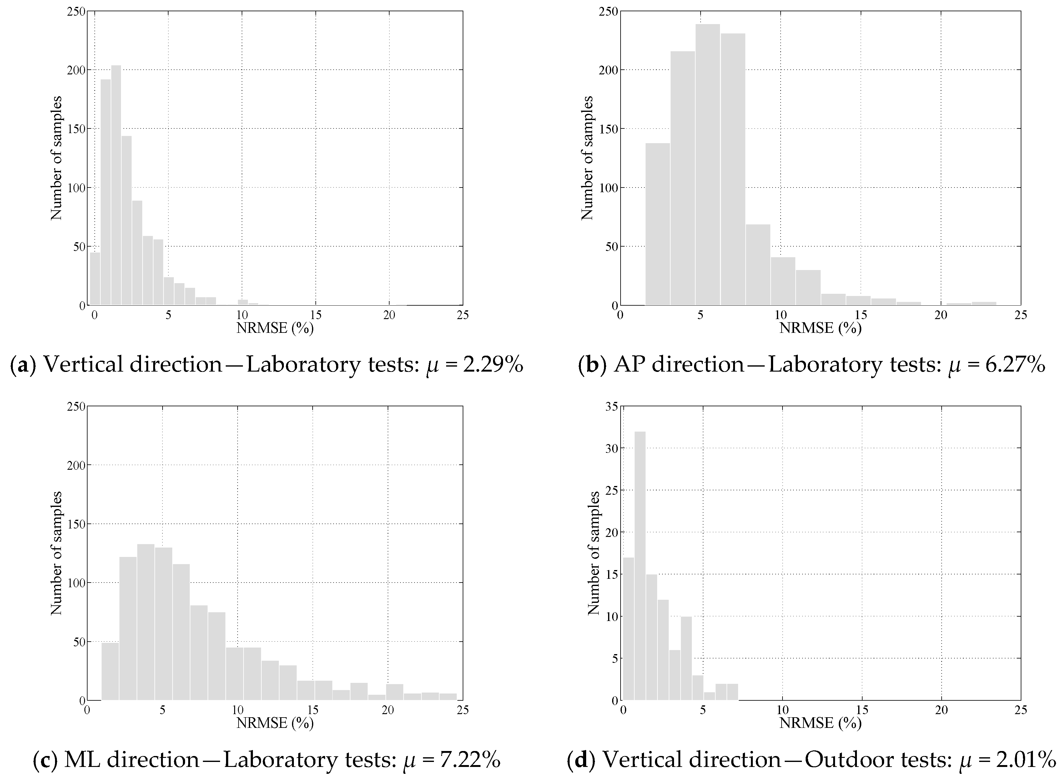
3.2.1. Performance of TPM in Laboratory Environment
3.2.2. Performance of TPM in Real-Life Environment
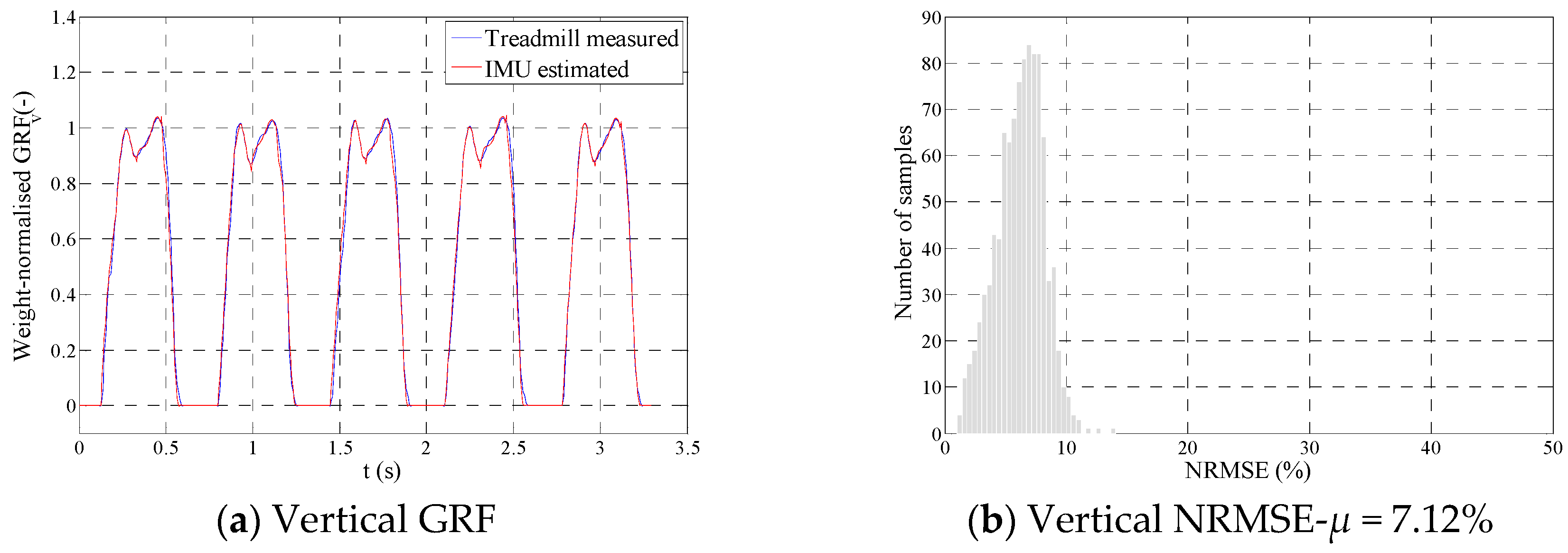
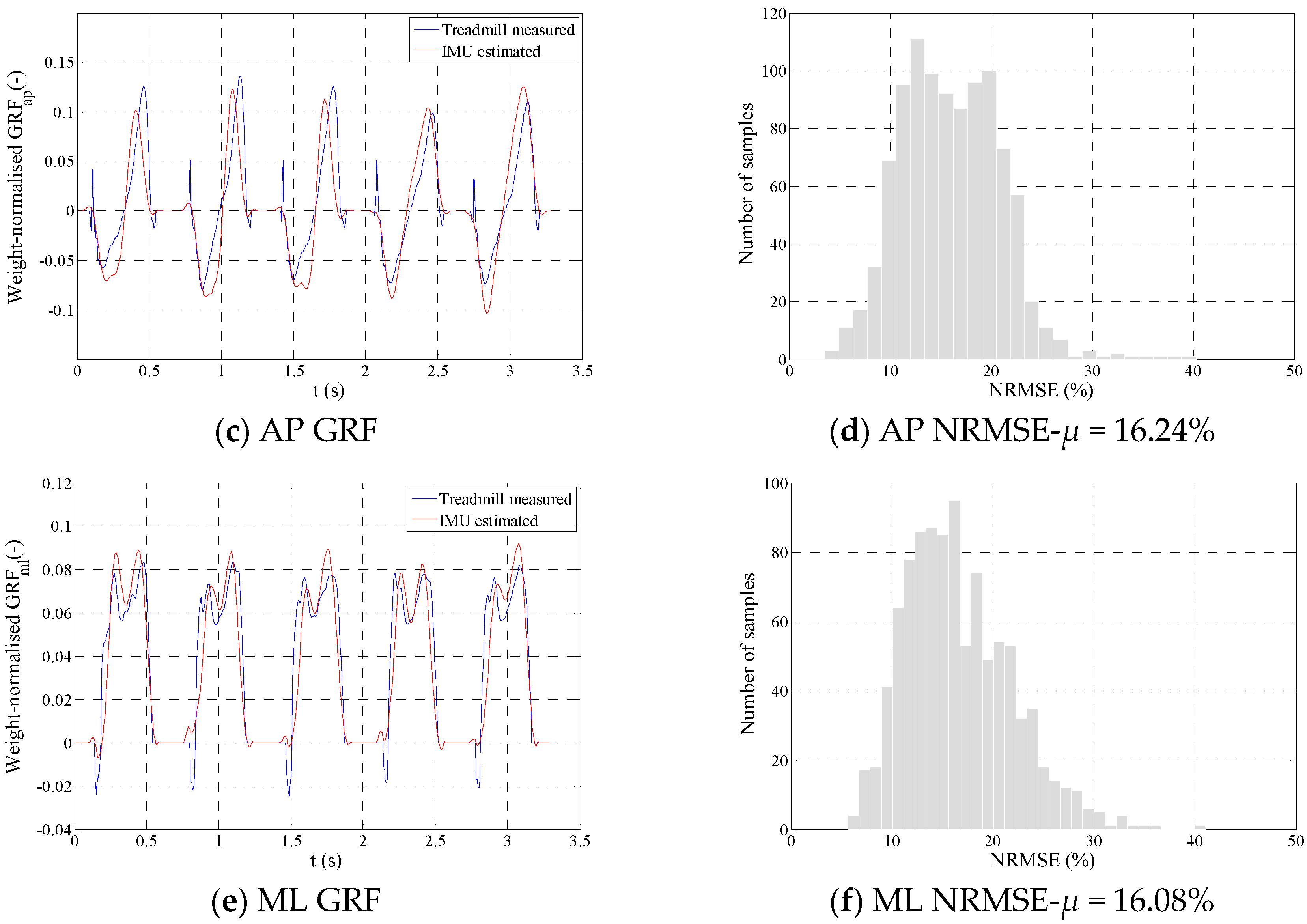
3.2.3. Application of TPM on IMU Data
4. Discussion
5. Conclusions
6. Declarations
Author Contributions
Funding
Conflicts of Interest
Abbreviations
| A, B, C, D, E, and A’, B’, C’, D’, E’ | Guiding points related to (Figure 3a) |
| ap | Anterior-posterior direction |
| Trajectory of center of plantar pressure | |
| DS | Double-support phase of the walking gait |
| Error in estimation of the total (Equation (2)) | |
| F, G, H, I, J, K, L and F’, G’, H’, I’, J’, K’, L’ | Guiding points related to (Figure 3c) |
| Total | Total (right and left foot) walking force |
| Left | Left foot walking force |
| Right | Right foot walking force |
| Left and right foot signals corresponding to half of a gait cycle and | |
| IMU | Inertial Measurement Unit |
| M, N, O, P, Q, R, S and M’, N’, O’, P’, Q’, R’, S’ | Guiding points related to (Figure 3e) |
| ml | Medial-lateral direction |
| n | Order of the polynomial curve |
| NRMSE | Peak-to-peak normalized root mean square error (Equation (1)) |
| Mean value of NRMSE values | |
| Standard deviation of NRMSE values | |
| Polynomial of degree n | |
| Probability Distribution Function | |
| Error scaling function (Equations (5) and (6)) | |
| SS | Single-support phase of the walking gait |
| Length of the resampled signals () | |
| Timing of guiding points (resampled to 100 points) | |
| TPM | Twin Polynomial Method |
| v | Vertical direction |
| Normalized amplitude of guiding points |
References
- Winter, D.A. The Biomechanics and Motor Control of Human Gait: Normal, Elderly and Pathological; University of Waterloo Press: Waterloo, ON, Canada, 1991. [Google Scholar]
- McDonald, M.G.; Zivanovic, S. Measuring dynamic force of a jumping person by monitoring their body kinematics. In Proceedings of the 11th International Conference on Recent Advances in Structural Dynamics (RASD), Pisa, Italy, 1–3 July 2013. [Google Scholar]
- Bocian, M.; Brownjohn, J.M.W.; Racic, V.; Hester, D.; Quattrone, A.; Monnickendam, R. A framework for experimental determination of localized vertical pedestrian forces on full-scale structures using wireless attitude and heading reference systems. J. Sound Vib. 2016, 376, 217–243. [Google Scholar] [CrossRef]
- Fluit, R.; Andersen, M.S.; Kolk, S.; Verdonschot, N.; Koopman, H.F.J.M. Prediction of ground reaction forces and moments during various activities of daily living. J. Biomech. 2014, 47, 2321–2329. [Google Scholar] [CrossRef] [PubMed]
- Koopman, B.; Grootenboer, H.J.; de Jongh, H.J. An inverse dynamics model for the analysis, reconstruction and prediction of bipedal walking. J. Biomech. 1995, 28, 1369–1376. [Google Scholar] [CrossRef]
- Vaughan, C.L.; Hay, J.G.; Andrews, J.G. Closed loop problems in biomechanics. Part II—An optimization approach. J. Biomech. 1982, 15, 201–210. [Google Scholar] [CrossRef]
- Davis, B.L.; Cavanagh, P.R. Decomposition of superimposed ground reaction forces into left and right force profiles. J. Biomech. 1993, 26, 593–597. [Google Scholar] [CrossRef]
- Quanbury, A.O.; Winter, D.A. Calculation of floor reaction forces from kinematic data during single support phase of human gait. In Proceedings of the 5th Canadian Medical and Biological Engineering Conference, Montreal, QC, Canada, 3–6 September 1974. [Google Scholar]
- Robertson, D.G.E.; Winter, D.A. Estimation of Ground Reaction Forces from Kinematics and Body Segment Parameters; Canadian Association of Sport Sciences: Vancouver, BC, Canada, 1979.
- McGhee, R.B. Mathematical models for dynamics and control of posture and gait. In Proceedings of the VII International Congress of Biomechanics, Warsaw, Poland, 18–21 September 1979. [Google Scholar]
- McGhee, R.B.; Koozekanani, S.H.; Gupta, S.; Cheng, I.S. Automatic estimation of joint forces and moments in human locomotion from television data. In Identification and System Parameter Estimation; Rajbman, E., Ed.; North-Holland: New York, NY, USA, 1978. [Google Scholar]
- Hardt, D.E.; Mann, R.W. A five body three-dimensional dynamic analysis of walking. J. Biomech. 1979, 13, 455–457. [Google Scholar] [CrossRef]
- Morecki, A.; Koozekanani, S.H.; McGhee, R.B. Reduced order dynamic models for computer analysis of human gait. In Proceedings of the IV International Symposium of Robots and Manipulators, Warsaw, Poland, 8–12 September 1981. [Google Scholar]
- Ren, L.; Jones, R.K.; Howard, D. Dynamic analysis of load carriage biomechanics during level walking. J. Biomech. 2005, 38, 853–863. [Google Scholar] [CrossRef] [PubMed]
- Ren, L.; Jones, R.K.; Howard, D. Whole body inverse dynamics over a complete gait cycle based only on measured kinematics. J. Biomech. 2008, 41, 2750–2759. [Google Scholar] [CrossRef] [PubMed]
- Ballaz, L.; Raison, M.; Detrembleur, C. Decomposition of the vertical ground reaction forces during gait on a single force plate. J. Musculoskelet. Neuronal Interact. 2013, 13, 236–243. [Google Scholar] [PubMed]
- Samadi, B.; Raison, M.; Detrembleur, C.; Ballaz, L. Real-time detection of reaction forces during gait on a ground equipped with a large force platform. In Proceedings of the Global Information Infrastructure and Networking Symposium (GIIS), Montreal, QC, Canada, 15–19 September 2014. [Google Scholar] [CrossRef]
- Villeger, D.; Costes, A.; Watier, B.; Moretto, P. An algorithm to decompose ground reaction forces and moments from a single force platform in walking gait. Med. Eng. Phys. 2014, 36, 1530–1535. [Google Scholar] [CrossRef] [PubMed]
- Meurisse, G.M.; Bastien, G.J. Determination of vertical ground reaction forces under each foot during walking. Comput. Methods Biomech. Biomed. Eng. 2014, 17, 110–111. [Google Scholar] [CrossRef] [PubMed]
- Karatsidis, A.; Bellusci, G.; Schepers, H.M.; de Zee, M.; Andersen, M.S.; Veltink, P.H. Estimation of Ground Reaction Forces and Moments during Gait Using Only Inertial Motion Capture. Sensors 2017, 17, 75. [Google Scholar] [CrossRef] [PubMed]
- Shahabpoor, E.; Pavic, A. Measurement of Walking Ground Reactions in Real-Life Environments: A Systematic Review of Techniques and Technologies. Sensors 2017, 17, 2085. [Google Scholar] [CrossRef] [PubMed]
- MathWorks. MATLAB and Statistics Toolbox Release 2016; MathWorks, Inc.: Natick, MA, USA, 2016. [Google Scholar]
- Tekscan. F-Scan® In-Shoe Analysis System Data Sheet. Available online: https://www.tekscan.com/sites/default/files/resources/MDL-F-Scan-Datasheet.pdf (accessed on 28 October 2016).
- APDM. Mobility Lab White Paper. Available online: http://www.apdm.com/wp-content/uploads/2015/10/Whitepaper1.pdf (accessed on 28 October 2016).
- Shahabpoor, E.; Pavic, A.; Brownjohn, J.M.W.; Billings, S.A.; Guo, L.; Bocian, M. Real-Life Measurement of Tri-Axial Walking Ground Reaction Forces Using Optimal Network of Wearable Inertial Measurement Units. IEEE Trans. Neural Syst. Rehabil. Eng. 2018, 26, 1243–1253. [Google Scholar] [CrossRef] [PubMed]


| n | Main Points | Guide Point/s | |||
|---|---|---|---|---|---|
| 5 | A | - | SS local minima | Total | |
| B | - | μ = 39.12; σ = 6.00; | Total | ||
| C | - | μ = 68.89; σ = 7.78; | |||
| - | D | μ = 0.79; σ = 0.58; | |||
| E | - | SS local minima | |||
| 5 | A | - | SS local minima | ||
| B | - | μ = 39.12; σ = 6.00; | |||
| C | - | μ = 68.89; σ = 7.78; | Total | ||
| - | D’ | μ = 0.79; σ = 0.58; | |||
| E | - | SS local minima | Total | ||
| 8 | F | - | SS zero crossing | ||
| G | - | Heel-strike of leading foot | Total | ||
| - | H | μ = 0.06; σ = 0.02; | |||
| - | I | μ = 56.04; σ = 4.58; | |||
| - | J | μ = −0.01; σ = 0.01; | |||
| K | - | Toe-off of trailing foot | |||
| L | - | SS zero crossing | |||
| 8 | F | - | SS zero crossing | ||
| G’ | - | Heel-strike of leading foot | |||
| - | H’ | μ = 0.02; σ = 0.06; | |||
| - | I’ | μ = 33.07; σ = 6.28; | |||
| - | J’ | μ = 0.03; σ = 0.02; | |||
| K’ | - | Toe-off of trailing foot | Total | ||
| L | - | SS zero crossing | |||
| 9 | M | - | SS local minima | Total | |
| N | - | Heel-strike of leading foot | Total | ||
| - | O | μ = −0.005; σ = 0.008; | |||
| - | P | μ = 54.70; σ = 6.32; | |||
| - | Q | μ = 0; σ = 0.016; | |||
| R | - | Toe-off of trailing foot | |||
| S | - | SS local maxima | |||
| 9 | M’ | - | SS local minima | ||
| N’ | - | Heel-strike of leading foot | |||
| - | O’ | μ = 0.008; σ = 0.013; | |||
| - | P’ | μ = 45.50; σ = 9.67; | |||
| - | Q’ | μ = 0.010; σ = 0.021; | |||
| R’ | - | Toe-off of trailing foot | Total | ||
| S’ | - | SS local maxima | Total |
© 2018 by the authors. Licensee MDPI, Basel, Switzerland. This article is an open access article distributed under the terms and conditions of the Creative Commons Attribution (CC BY) license (http://creativecommons.org/licenses/by/4.0/).
Share and Cite
Shahabpoor, E.; Pavic, A. Estimation of Tri-Axial Walking Ground Reaction Forces of Left and Right Foot from Total Forces in Real-Life Environments. Sensors 2018, 18, 1966. https://doi.org/10.3390/s18061966
Shahabpoor E, Pavic A. Estimation of Tri-Axial Walking Ground Reaction Forces of Left and Right Foot from Total Forces in Real-Life Environments. Sensors. 2018; 18(6):1966. https://doi.org/10.3390/s18061966
Chicago/Turabian StyleShahabpoor, Erfan, and Aleksandar Pavic. 2018. "Estimation of Tri-Axial Walking Ground Reaction Forces of Left and Right Foot from Total Forces in Real-Life Environments" Sensors 18, no. 6: 1966. https://doi.org/10.3390/s18061966
APA StyleShahabpoor, E., & Pavic, A. (2018). Estimation of Tri-Axial Walking Ground Reaction Forces of Left and Right Foot from Total Forces in Real-Life Environments. Sensors, 18(6), 1966. https://doi.org/10.3390/s18061966