Two-Phase Framework for Indoor Positioning Systems Using Visible Light †

Abstract
1. Introduction
2. Visible Light Positioning Systems
3. Two-Phase Positioning Framework
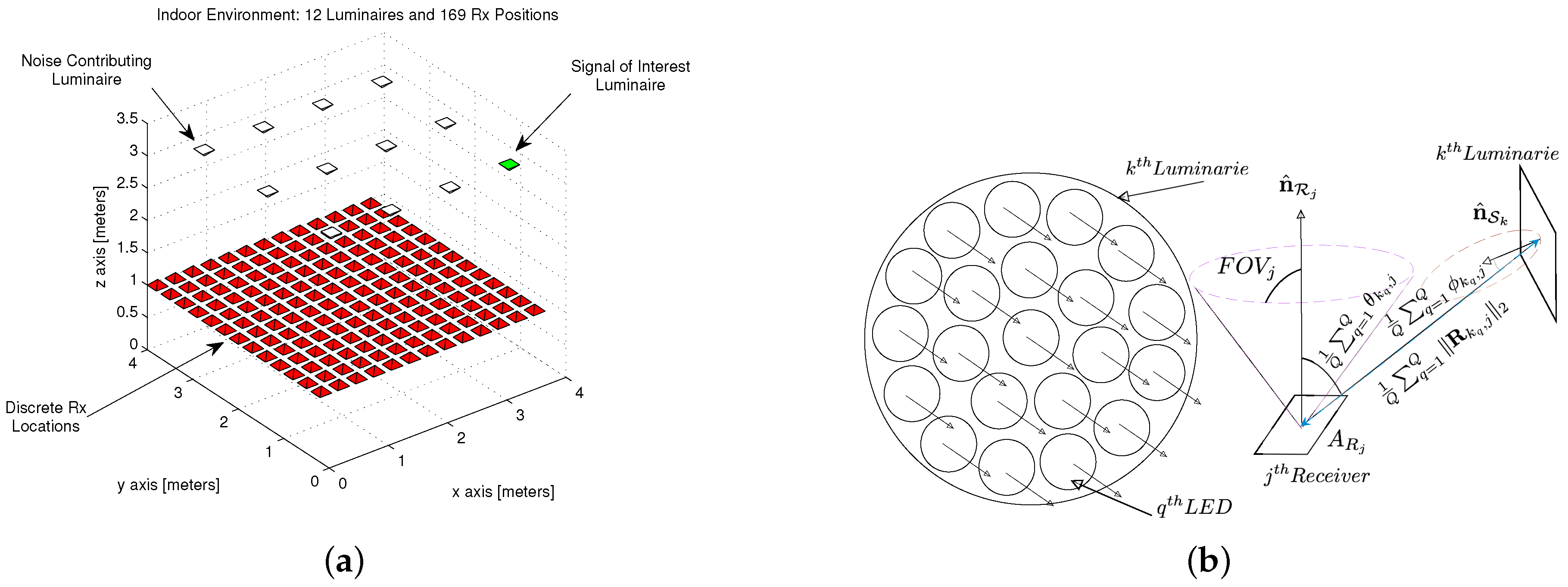
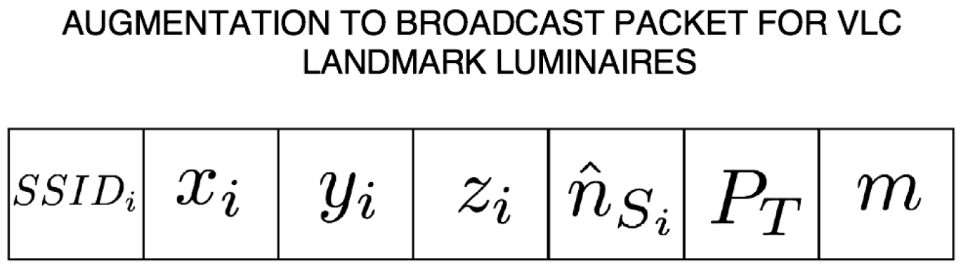
3.1. Model Framework
3.2. Coarse Phase
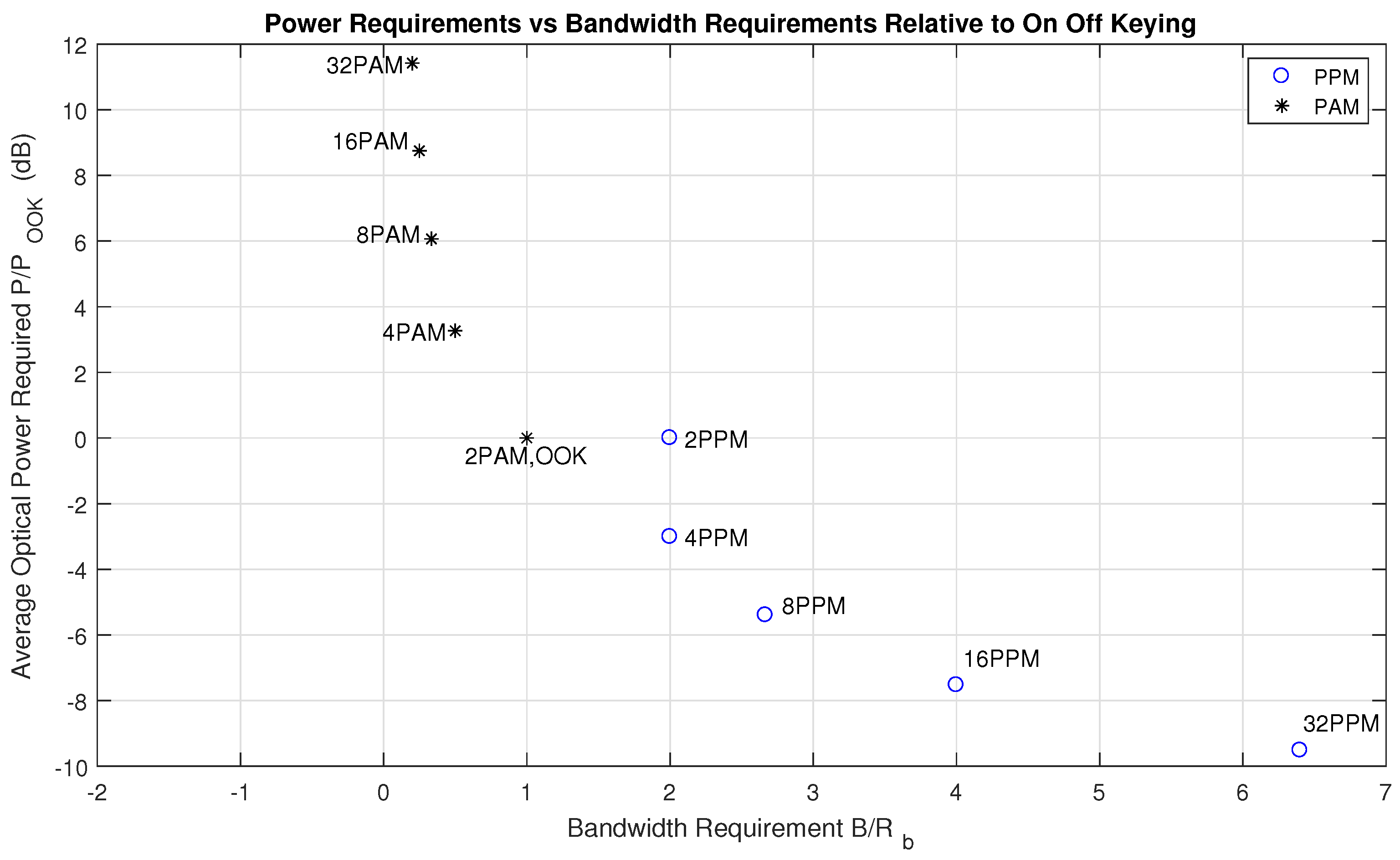
3.2.1. Modulations
Pulsed Modulation
Muti-Carrier Modulations
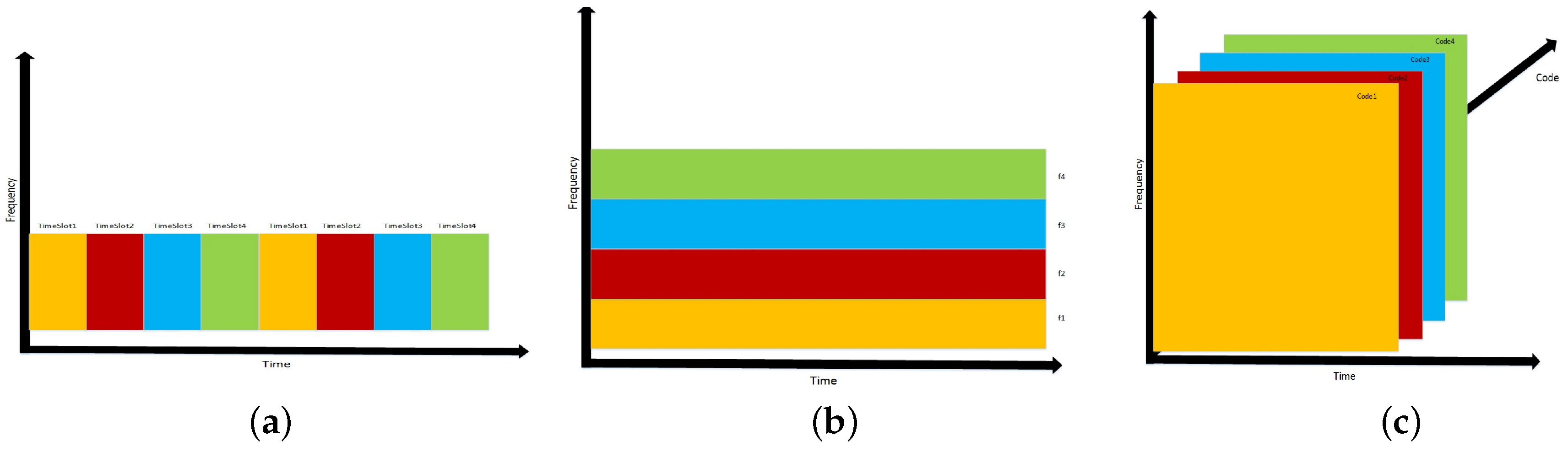
3.2.2. Multiple Access
Time Division Multiplexing (TDM)
Frequency Division Multiplexing (FDM) & Wavelength Division Multiplexing (WDM)
Code Division Multiplexing (CDM)
3.3. Fine Phase
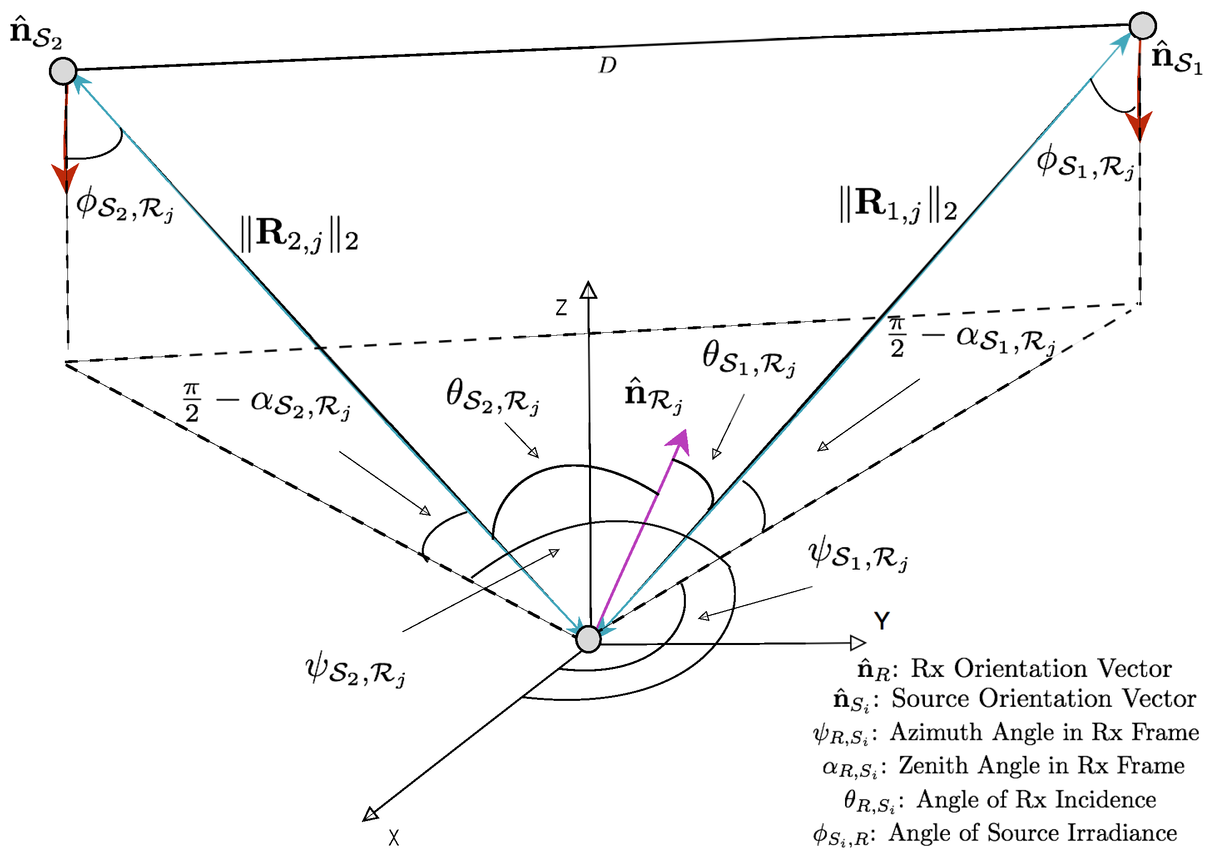
3.4. Fine Phase-Triangulation Based Positioning Using AoA
3.5. Fine Phase-Trilateration Based Positioning Using ToF or RSS
- RF Channel: , where is the gain of the transmit antenna, is the gain of the receive antenna, is the wavelength of the RF signal.
- VLC Channel: , where angle of emission dependent transmit optics, is the effective area of the photodetector, is the angle of incidence dependent concentration optics at the receiver.
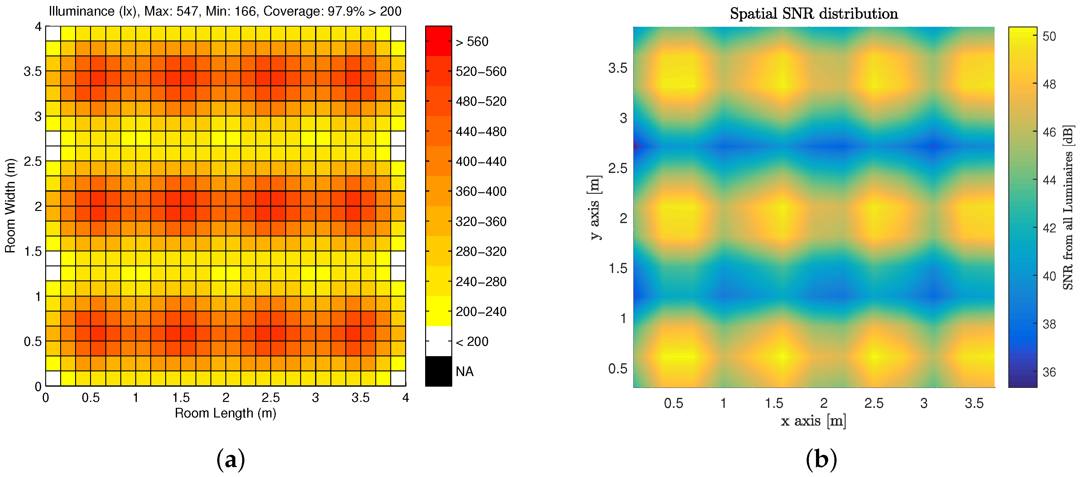
4. Results
4.1. Coarse
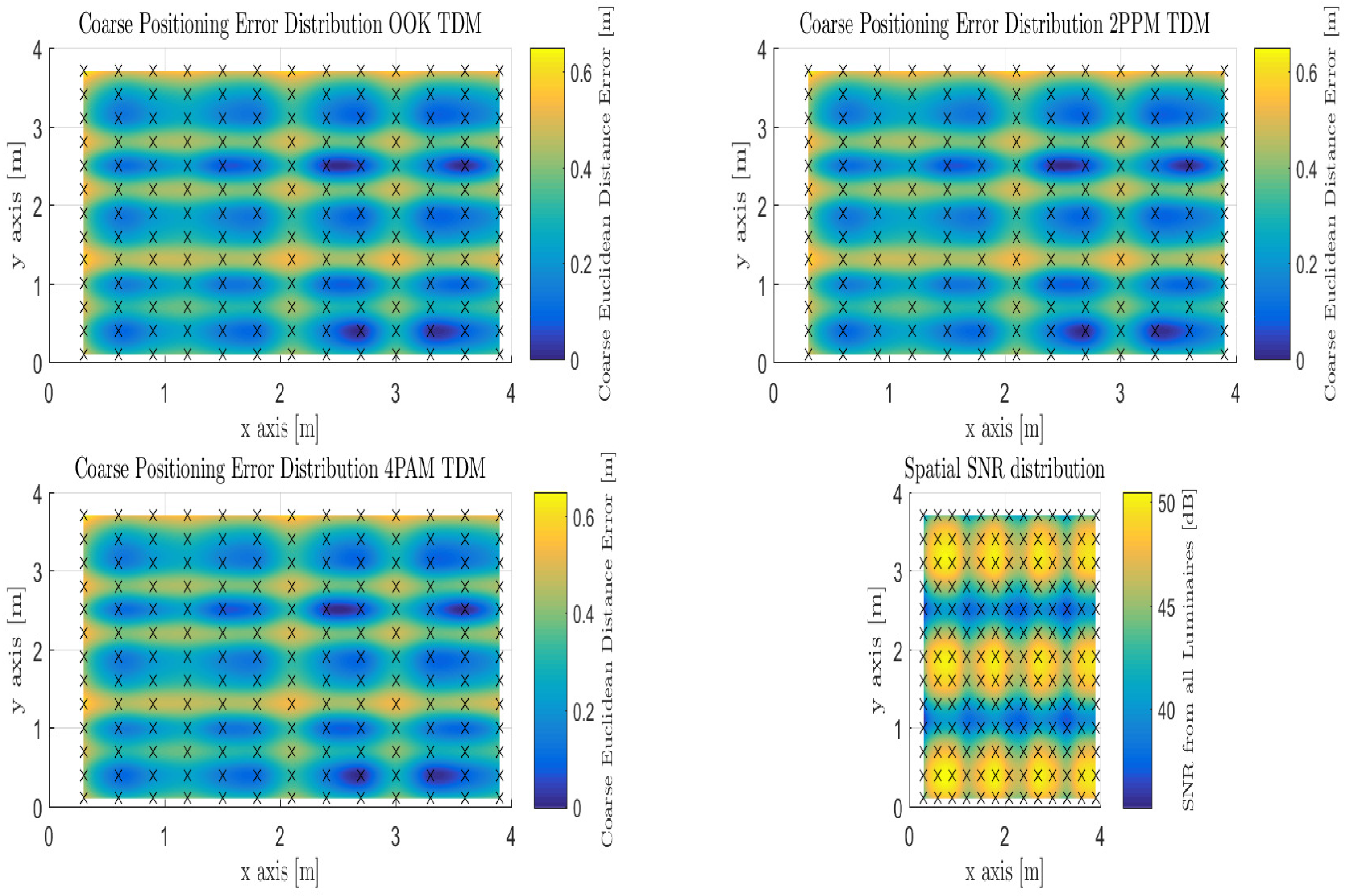
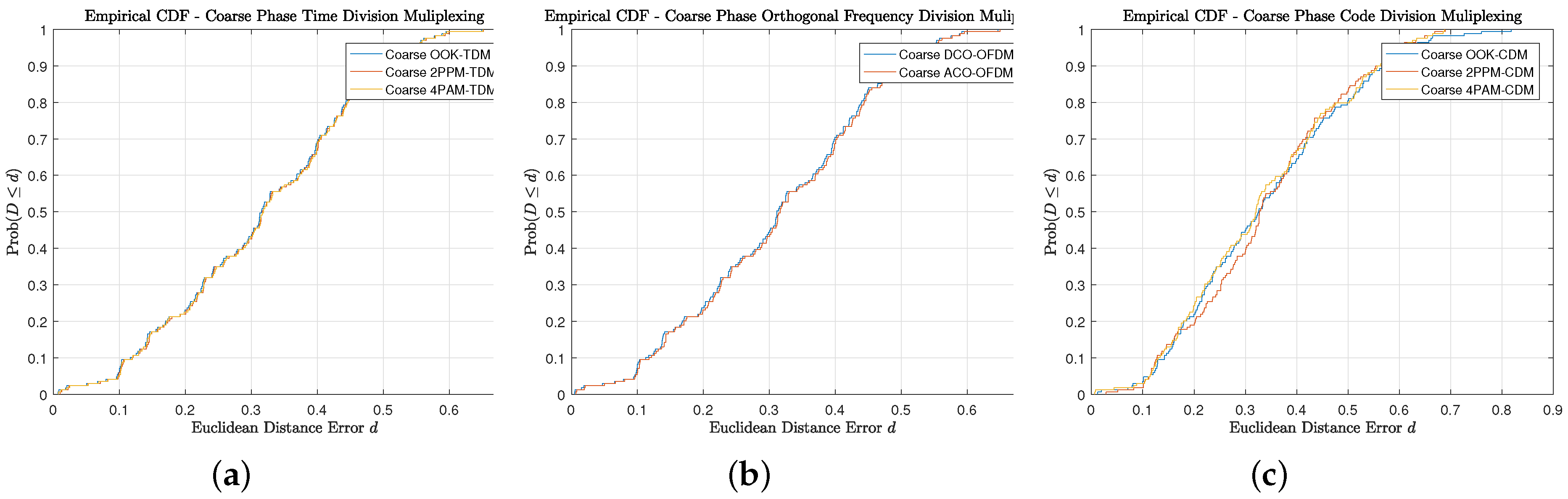
4.1.1. Coarse Phase-Proximity-Based Positioning with Time Division Multiplexing
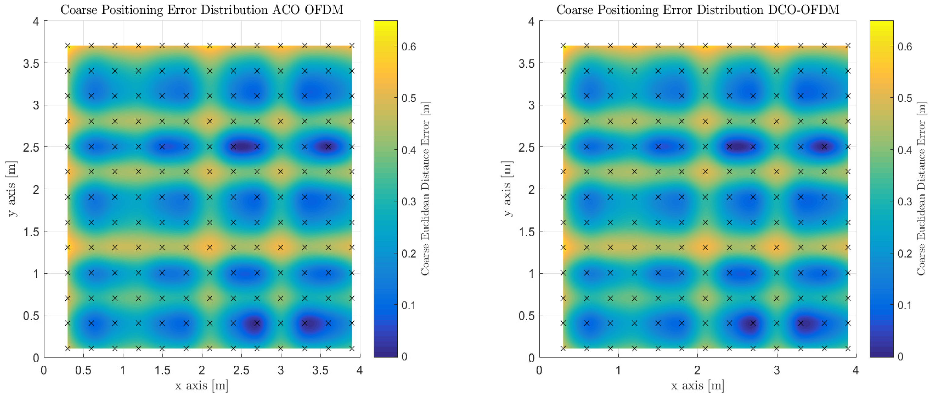
4.1.2. Coarse Phase-Proximity-Based Positioning with Frequency Division Multiplexing
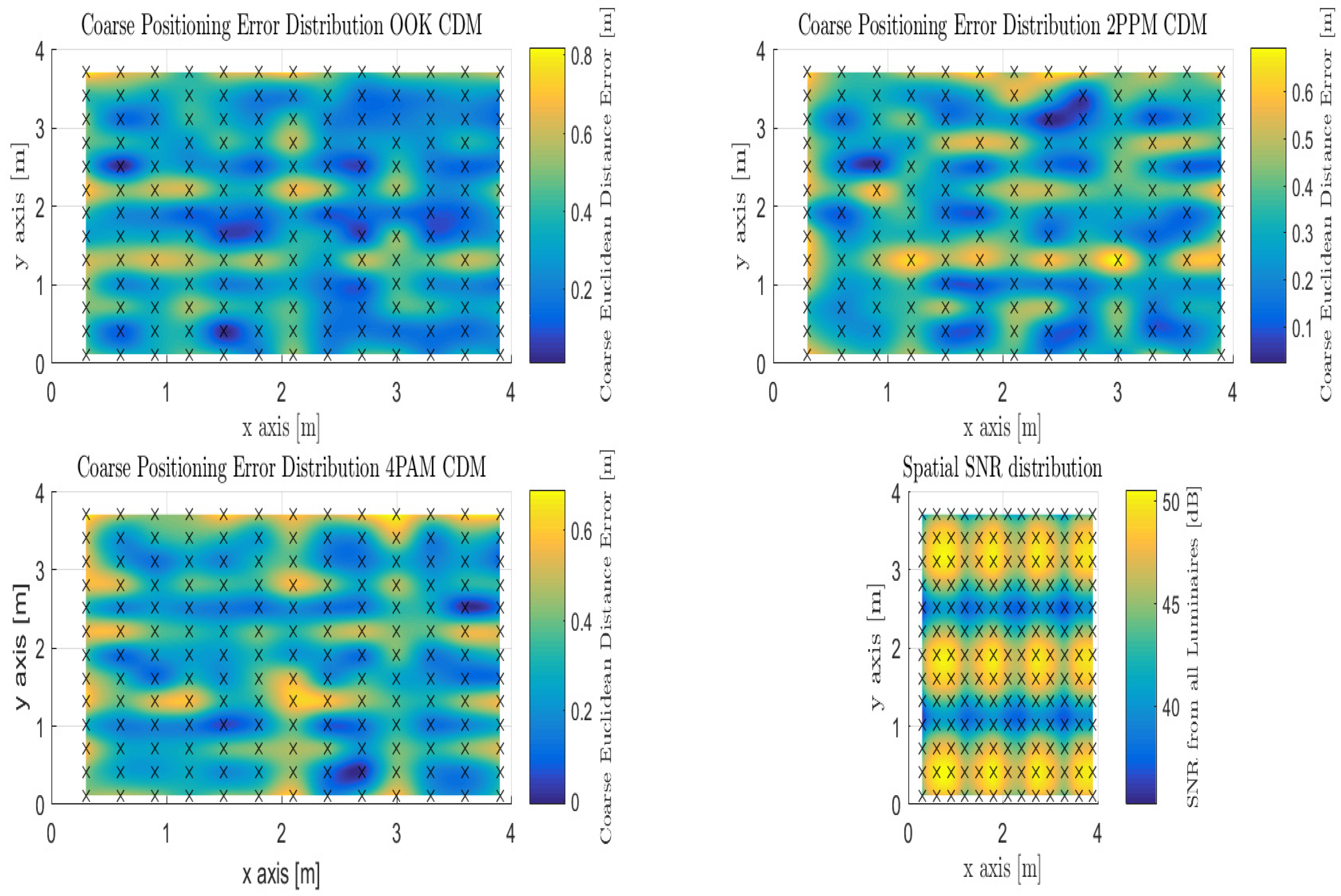
4.1.3. Coarse Phase-Proximity-Based Positioning with Code Division Multiplexing
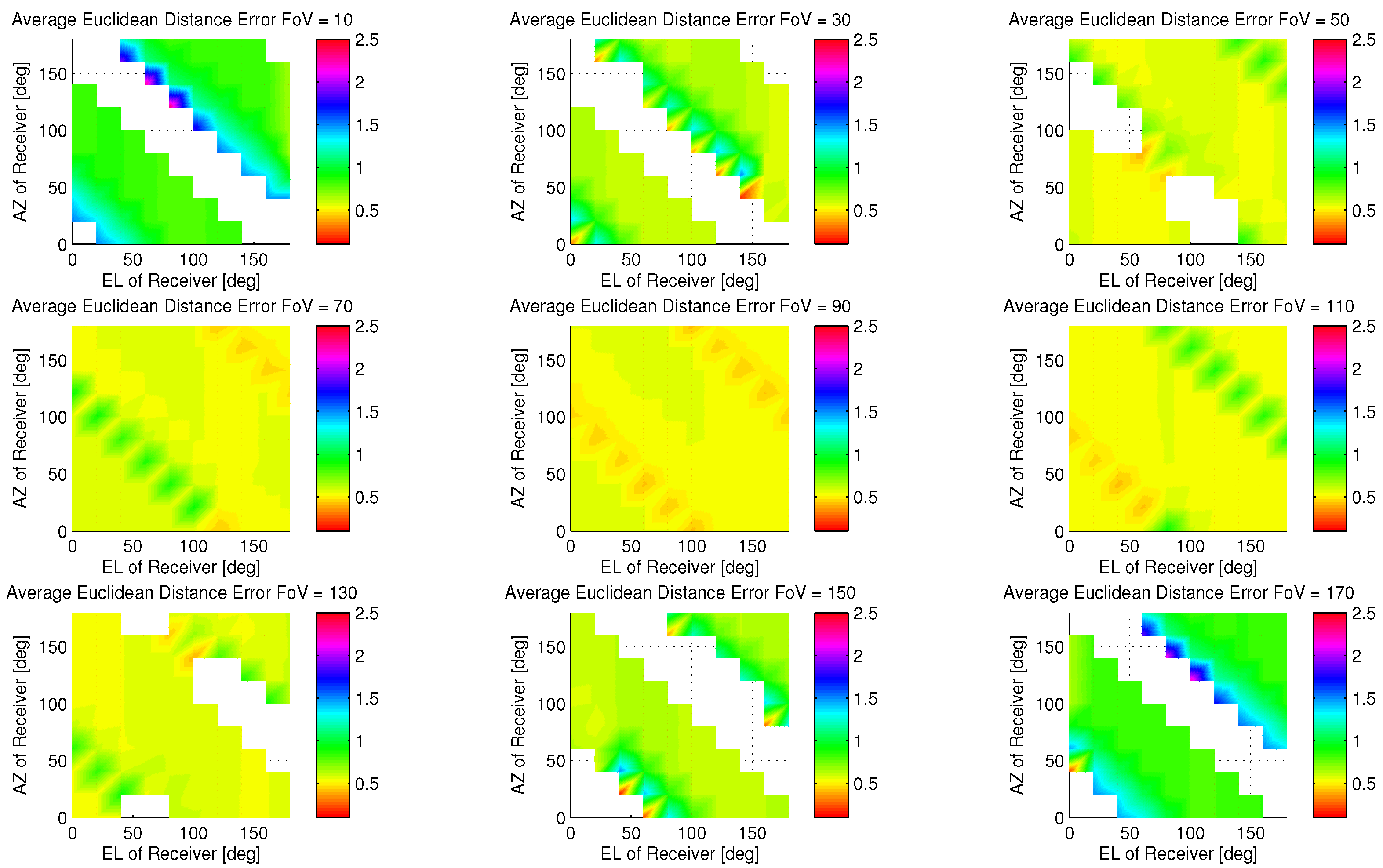
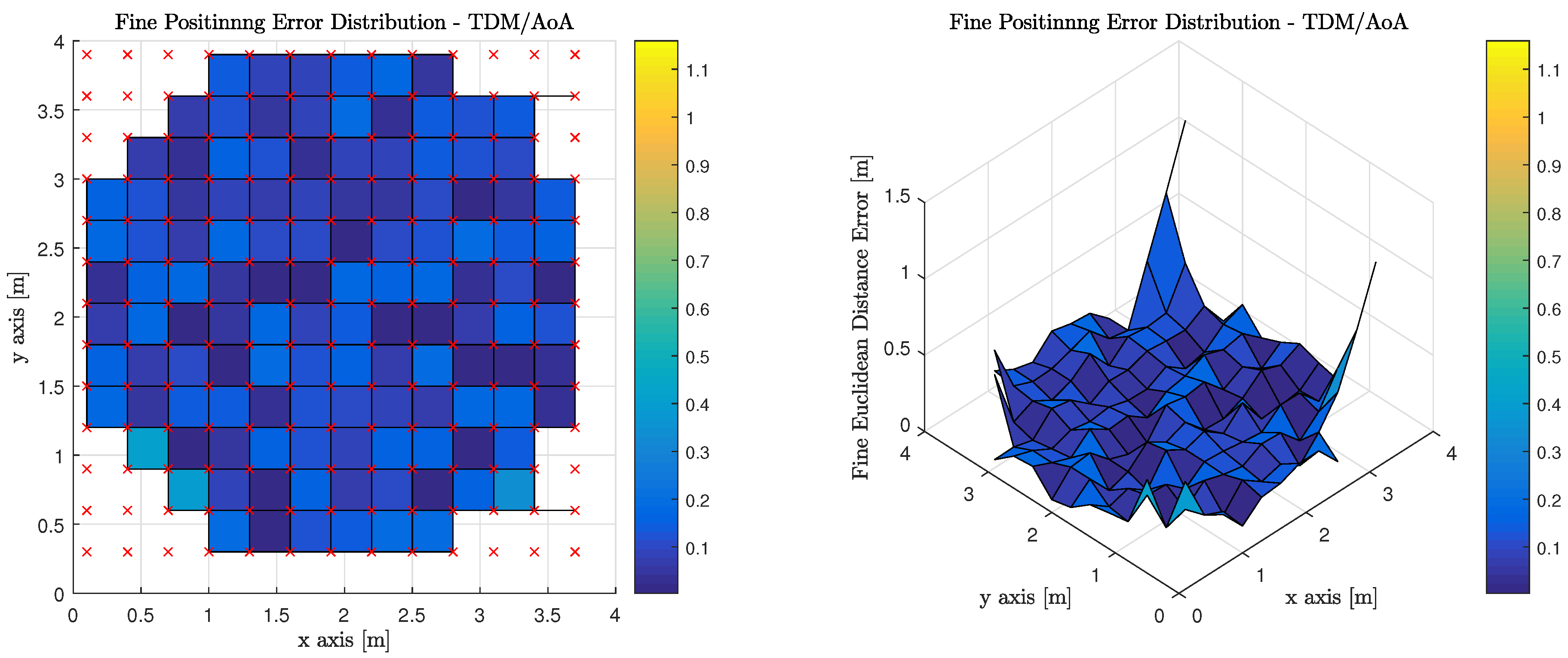
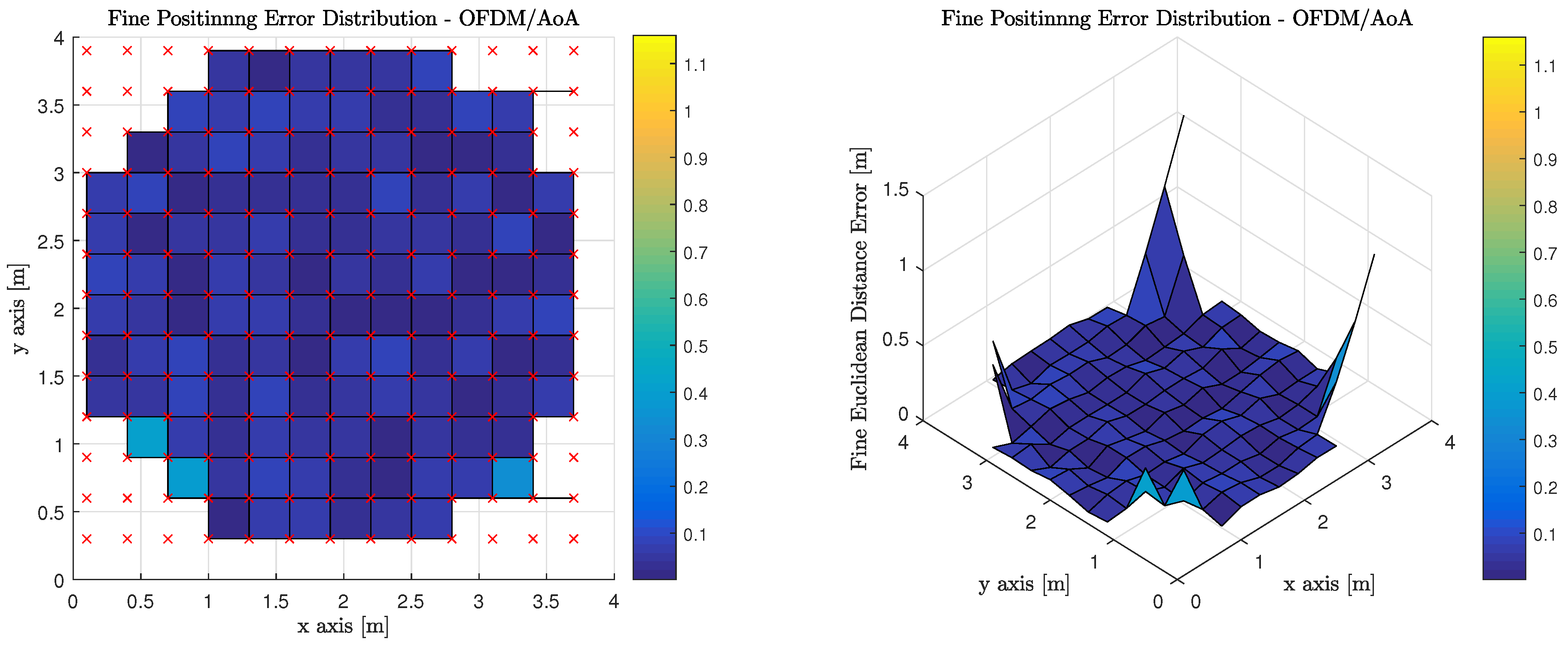
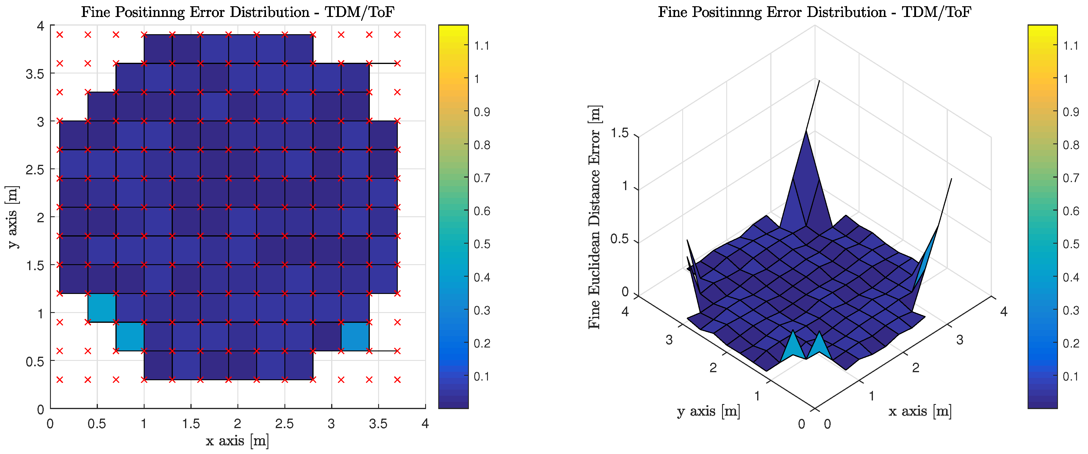
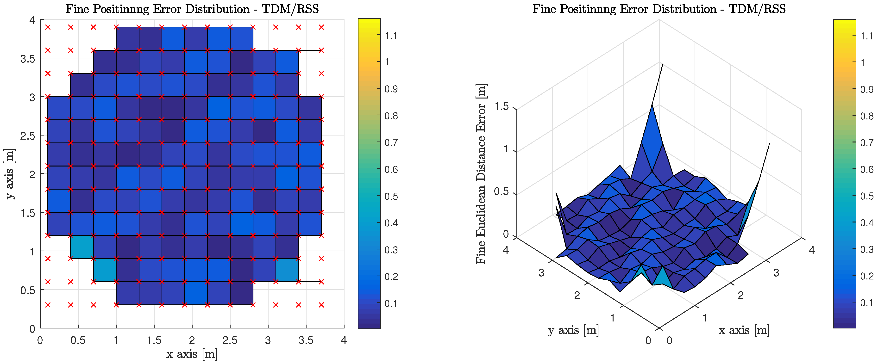
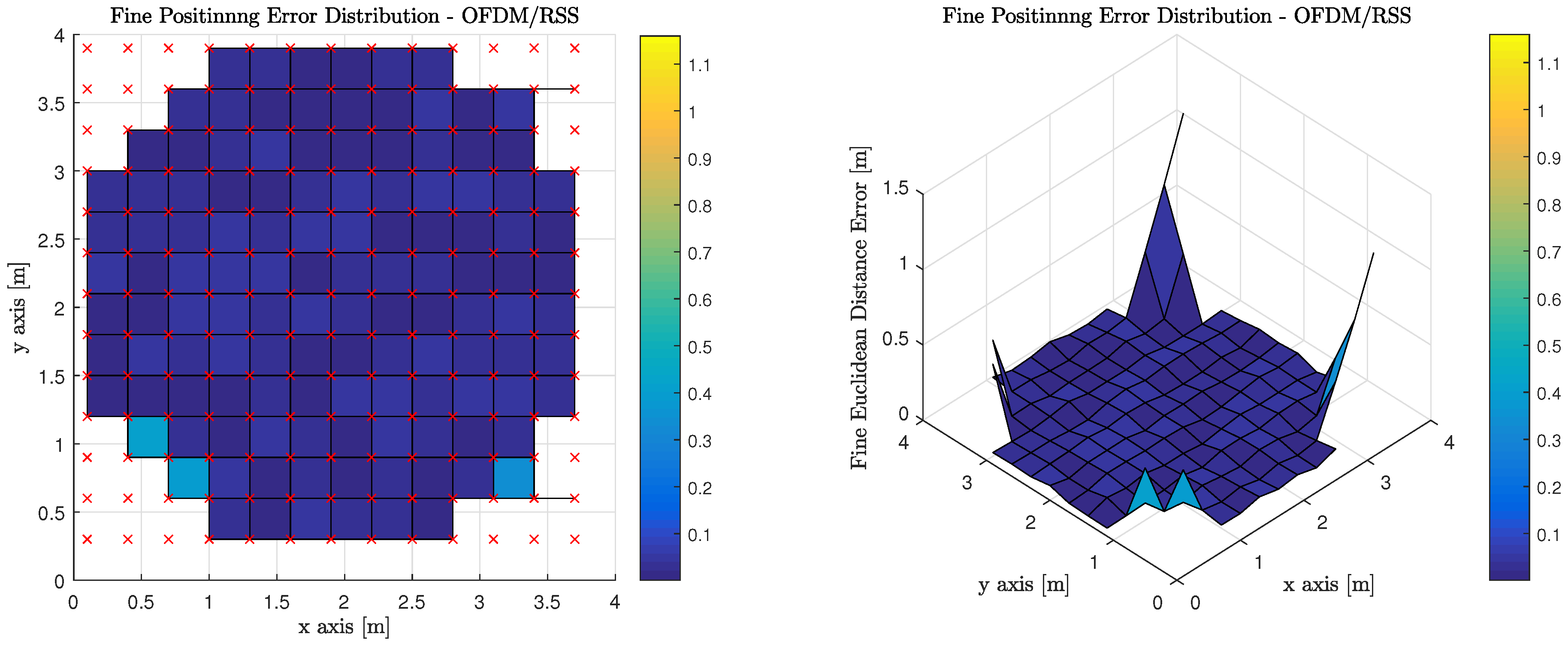
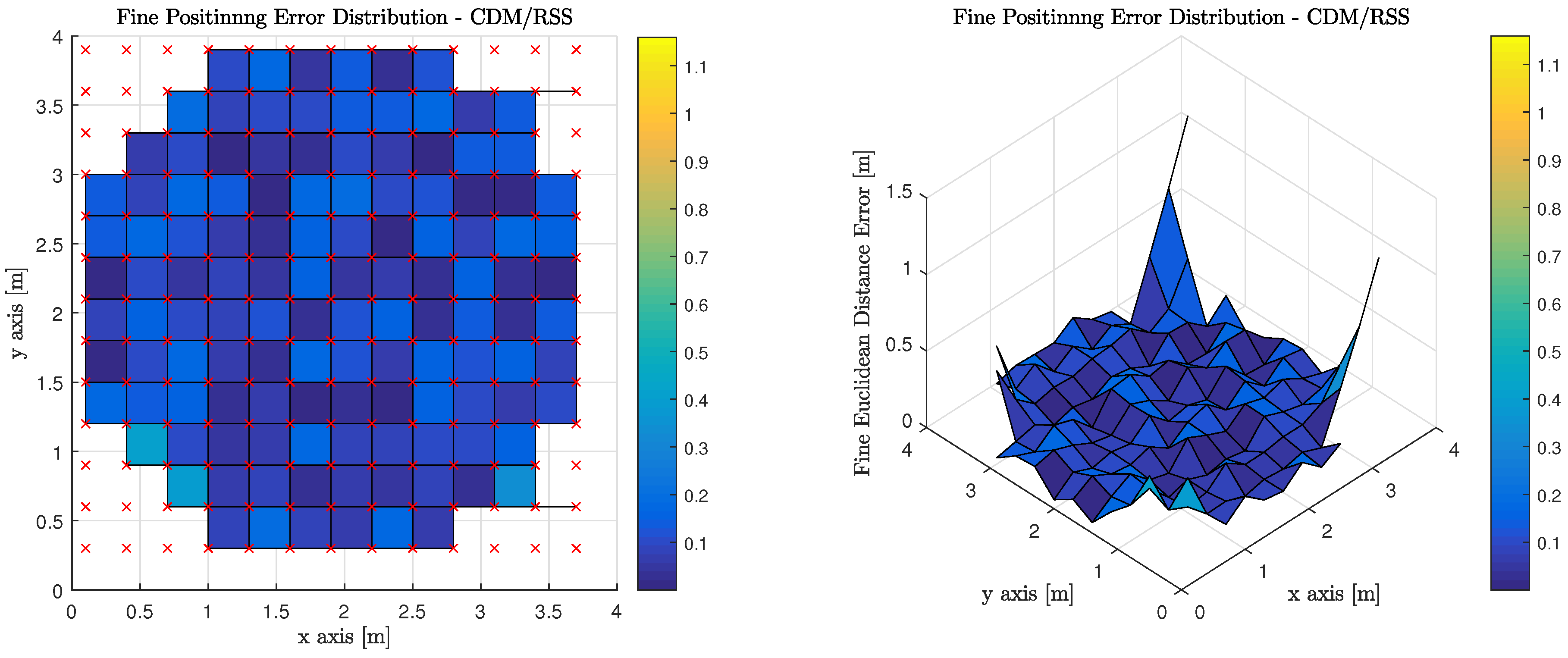
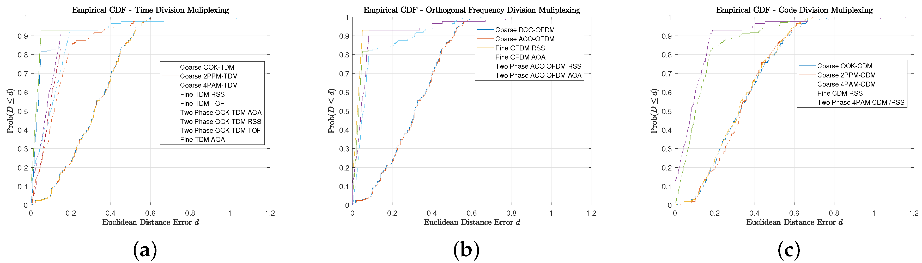
4.2. Fine
4.3. Two-Phase
5. Conclusions
Author Contributions
Funding
Acknowledgments
Conflicts of Interest
References
- Armstrong, J.; Sekercioglu, Y.A.; Neild, A. Visible light positioning: A roadmap for international standardization. IEEE Commun. Mag. 2013, 51, 68–73. [Google Scholar] [CrossRef]
- Luo, J.; Fan, L.; Li, H. Indoor Positioning Systems Based on Visible Light Communication: State of the Art. IEEE Commun. Sur. Tutor. 2017, 19, 2871–2893. [Google Scholar] [CrossRef]
- Do, T.H.; Yoo, M. An in-Depth Survey of Visible Light Communication Based Positioning Systems. Sensors 2016, 16, 678. [Google Scholar] [CrossRef] [PubMed]
- Prince, G.B.; Little, T.D. A two phase hybrid RSS/AoA algorithm for indoor device localization using visible light. In Proceedings of the 2012 IEEE Global Communications Conference (GLOBECOM), Anaheim, CA, USA, 3–7 December 2012; pp. 3347–3352. [Google Scholar]
- Liu, X.; Makino, H.; Mase, K. Improved indoor location estimation using fluorescent light communication system with a nine-channel receiver. IEICE Trans. Commun. 2010, 93, 2936–2944. [Google Scholar] [CrossRef]
- Liu, X.; Makino, H.; Kobayashi, S.; Maeda, Y. Research of practical indoor guidance platform using fluorescent light communication. IEICE Trans. Commun. 2008, 91, 3507–3515. [Google Scholar] [CrossRef]
- Zhang, W.; Kavehrad, M. Comparison of VLC-Based Indoor Positioning Techniques. Proc. SPIE 2013, 8645. [Google Scholar] [CrossRef]
- Cossu, G.; Presi, M.; Corsini, R.; Choudhury, P.; Khalid, A.M.; Ciaramella, E. A Visible Light localization aided Optical Wireless system. In Proceedings of the 2011 IEEE Globecom Workshops, Houston, TX, USA, 5–9 December 2011; pp. 802–807. [Google Scholar]
- Sertthin, C.; Tsuji, E.; Nakagawa, M.; Kuwano, S.; Watanabe, K. A switching estimated receiver position scheme for visible light based indoor positioning system. In Proceedings of the 2009 4th International Symposium on Wireless Pervasive Computing, Melbourne, Australia, 11–13 February 2009; pp. 1–5. [Google Scholar]
- Sertthin, C. An Indoor Positioning Architecture Based on Visible Light Communication and Multiband Received Signal Strength Fingerprinting. Ph.D. Thesis, Keio University, Tokyo, Japan, 2011. [Google Scholar]
- Yasir, M.; Ho, S.W.; Vellambi, B.N. Indoor localization using visible light and accelerometer. In Proceedings of the 2013 IEEE Global Communications Conference (GLOBECOM), Atlanta, GA, USA, 9–13 December 2013; pp. 3341–3346. [Google Scholar]
- Yasir, M.; Ho, S.W.; Vellambi, B.N. Indoor positioning system using visible light and accelerometer. J. Lightwave Technol. 2014, 32, 3306–3316. [Google Scholar] [CrossRef]
- Won, Y.Y.; Yang, S.H.; Kim, D.H.; Han, S.K. Three-dimensional optical wireless indoor positioning system using location code map based on power distribution of visible light emitting diode. IET Optoelectron. 2013, 7, 77–83. [Google Scholar] [CrossRef]
- Gu, W.; Zhang, W.; Kavehrad, M.; Feng, L. Three-dimensional light positioning algorithm with filtering techniques for indoor environments. Opt. Eng. 2014, 53, 107107. [Google Scholar] [CrossRef]
- Nguyen, T.; Jang, Y.M. Highly Accurate Indoor Three-Dimensional Localization Technique in Visible Light Communication Systems. J. Korea Inf. Commun. Soc. 2013, 38, 775–780. [Google Scholar] [CrossRef]
- Jeong, E.M.; Yang, S.H.; Kim, H.S.; Han, S.K. Tilted receiver angle error compensated indoor positioning system based on visible light communication. Electron. Lett. 2013, 49, 890–892. [Google Scholar] [CrossRef]
- Kim, H.S.; Kim, D.R.; Yang, S.H.; Son, Y.H.; Han, S.K. An indoor visible light communication positioning system using a RF carrier allocation technique. J. Lightwave Technol. 2013, 31, 134–144. [Google Scholar] [CrossRef]
- Kim, H.S.; Kwon, D.H.; Yang, S.H.; Son, Y.H.; Han, S.K. Channel Assignment Technique for RF Frequency Reuse in CA-VLC-Based Accurate Optical Indoor Localization. J. Lightwave Technol. 2014, 32, 2544–2555. [Google Scholar] [CrossRef]
- Do, T.H.; Hwang, J.; Yoo, M. TDoA based indoor visible light positioning systems. In Proceedings of the 2013 Fifth International Conference on Ubiquitous and Future Networks (ICUFN), Da Nang, Vietnam, 2–5 July 2013; pp. 456–458. [Google Scholar]
- Zhang, W.; Chowdhury, M.S.; Kavehrad, M. Asynchronous indoor positioning system based on visible light communications. Opt. Eng. 2014, 53, 045105. [Google Scholar] [CrossRef]
- Lou, P.; Zhang, H.; Zhang, X.; Yao, M.; Xu, Z. Fundamental Analysis for Indoor Visible Light Positioning System. In Proceedings of the 2012 1st IEEE International Conference on Communications in Communications in China Workshops (ICCC), Beijing, China, 15–17 August 2012; pp. 59–63. [Google Scholar]
- Jung, S.Y.; Hann, S.; Park, C.S. TDOA-based optical wireless indoor localization using LED ceiling lamps. IEEE Trans. Consumer Electron. 2011, 57, 1592–1597. [Google Scholar] [CrossRef]
- Nah, J.; Parthiban, R.; Jaward, M.H. Visible Light Communications localization using TDOA-based coherent heterodyne detection. In Proceedings of the 2013 IEEE 4th International Conference on Photonics (ICP), Melaka, Malaysia, 28–30 October 2013; pp. 247–249. [Google Scholar]
- Luo, P.; Zhang, M.; Zhang, X.; Cai, G.; Han, D.; Li, Q. An indoor visible light communication positioning system using dual-tone multi-frequency technique. In Proceedings of the 2013 2nd International Workshop on Optical Wireless Communications (IWOW), Newcastle upon Tyne, UK, 21 October 2013; pp. 25–29. [Google Scholar]
- Panta, K.; Armstrong, J. Indoor localisation using white LEDs. Inst. Eng. Technol. Electron. Lett. 2012, 48, 228–230. [Google Scholar] [CrossRef]
- Jia, Z. A Visible Light Communication Based Hybrid Positioning Method for Wireless Sensor Networks. In Proceedings of the 2012 Second International Conference on Intelligent System Design and Engineering Application (ISDEA), Sanya, China, 6–7 January 2012; pp. 1367–1370. [Google Scholar]
- Wang, T.Q.; Sekercioglu, Y.A.; Neild, A.; Armstrong, J. Position accuracy of time-of-arrival based ranging using visible light with application in indoor localization systems. J. Lightwave Technol. 2013, 31, 3302–3308. [Google Scholar] [CrossRef]
- Vegni, A.M.; Biagi, M. An indoor localization algorithm in a small-cell LED-based lighting system. In Proceedings of the 2012 International Conference on Indoor Positioning and Indoor Navigation (IPIN), Sydney, Australia, 13–15 November 2012; pp. 1–7. [Google Scholar]
- Kail, G.; Maechler, P.; Preyss, N.; Burg, A. Robust asynchronous indoor localization using LED lighting. In Proceedings of the 2014 IEEE International Conference on Acoustics, Speech and Signal Processing (ICASSP), Florence, Italy, 4–9 May 2014; pp. 1866–1870. [Google Scholar]
- Jung, S.Y.; Lee, S.R.; Park, C.S. Indoor location awareness based on received signal strength ratio and time division multiplexing using light-emitting diode light. Opt. Eng. 2014, 53, 016106. [Google Scholar] [CrossRef]
- Jung, S.Y.; Choi, C.K.; Heo, S.H.; Lee, S.R.; Park, C.S. Received signal strength ratio based optical wireless indoor localization using light emitting diodes for illumination. In Proceedings of the 2013 IEEE International Conference on Consumer Electronics (ICCE), Las Vegas, NV, USA, 11–14 January 2013. [Google Scholar]
- Jung, S.Y.; Park, C.S. Lighting LEDs based Indoor Positioning System using Received Signal Strength Ratio. In Proceedings of 3DSA2013; Springer: Berlin, Germany, 2016; Volume 8, p. 5. [Google Scholar]
- Hann, S.; Kim, J.H.; Jung, S.Y.; Park, C.S. White LED ceiling lights positioning systems for optical wireless indoor applications. In Proceedings of the 36th European Conference and Exhibition on Optical Communication, Torino, Italy, 19–23 September 2010. [Google Scholar]
- Girod, L.; Estrin, D. Robust range estimation using acoustic and multimodal sensing. In Proceedings of the 2001 IEEE/RSJ International Conference on Intelligent Robots and Systems, Maui, HI, USA, 29 October–3 November 2001; Volume 3, pp. 1312–1320. [Google Scholar]
- Abedi, A.; Chen, J. A Hybrid Framework for Radio Localization in Broadband Wireless Systems. In Proceedings of the 2010 IEEE Global Telecommunications Conference, Miami, FL, USA, 6–10 December 2010; p. 1. [Google Scholar]
- Rahaim, M.; Vegni, A.; Little, T. A hybrid radio frequency and broadcast visible light communication system. In Proceedings of the 2011 IEEE GLOBECOM Workshops (GC Wkshps), Houston, TX, USA, 5–9 December 2011; pp. 792–796. [Google Scholar]
- Lee, Y.; Baang, S.; Park, J.; Zhou, Z.; Kavehrad, M. Hybrid Positioning with Lighting LEDs and Zigbee Multihop Wireless Network. Proc. SPIE 2012, 8282. [Google Scholar] [CrossRef]
- Rahaim, M.; Borogovac, T.; Carruthers, J. CandlES: Communication and lighting emulation software. In Proceedings of the Fifth ACM International Workshop on Wireless Network Testbeds, Experimental Evaluation and Characterization, Chicago, IL, USA, 20–24 September 2010; ACM: New York, NY, USA, 2010; pp. 9–14. [Google Scholar]
- Shen, J.; Oda, Y. Direction estimation for cellular enhanced cell-ID positioning using multiple sector observations. In Proceedings of the 2010 International Conference on Indoor Positioning and Indoor Navigation (IPIN), Zurich, Switzerland, 15–17 September 2010; pp. 1–6. [Google Scholar]
- De Lausnay, S.; De Strycker, L.; Goemaere, J.P.; Stevens, N.; Nauwelaers, B. Influence of MAI in a CDMA VLP system. In Proceedings of the 2015 International Conference on Indoor Positioning and Indoor Navigation (IPIN), Banff, AB, Canada, 13–16 October 2015; pp. 1–9. [Google Scholar]
- Cohen, C.; Koss, F. Comprehensive study of three object triangulation. Proc. SPIE 1993, 1831. [Google Scholar] [CrossRef]
- Bishop, A.; Anderson, B.; Fidan, B.; Pathirana, P.; Mao, G. Bearing-only localization using geometrically constrained optimization. IEEE Trans. Aerosp. Electron. Syst. 2009, 45, 308–320. [Google Scholar] [CrossRef]
- Linde, H. On Aspects of Indoor Localization. Ph.D. Thesis, Universität Dortmund, Dortmund, Germany, 2006. [Google Scholar]
- Manolakis, D. Efficient solution and performance analysis of 3-D position estimation by trilateration. IEEE Trans. Aerosp. Electron. Syst. 1996, 32, 1239–1248. [Google Scholar] [CrossRef]
- Coope, I. Reliable computation of the points of intersection of n spheres in n-dimensional real space. ANZIAM J. 2000, 42, C461–C477. [Google Scholar] [CrossRef]


| Parameter | Value | Units |
|---|---|---|
| Optical Tx Power | 1.924 | W |
| Lambertian Mode | 1 | - |
| Effective Area of Rx | 0.81 | |
| Electron Charge | C | |
| Background Light Current | A | |
| Speed of Light | m/s | |
| Noise PSD | W/Hz | |
| Optical / Electrical Efficiency | 0.53 | - |
| Source Orientation Vector | - | |
| Rx Azimuth Angle | rad | |
| Rx Elevation Angle | rad | |
| Rx Orientation Vector | ||
| Vertical Range | 2.2 | m |
| Symbol Rate | 20 | symbols/s |
| Source Bandwidth | 20 | MHz |
| Field of View | rad | |
| Wall Reflectivity | 0.6 | - |
| Coarse Phase Multiplexing Scheme | Benefits | Drawbacks |
|---|---|---|
| OFDM | Better suited for high data rate communication, Asynchronous | Complex Modulator and Demodulator |
| TDM | Simplistic | Requires Network Infrastructure, Highly Accurate Clocks, Synchronous |
| CDM | Asynchronous | Multiple Access Interference, Codes are not fully orthogonal |
| Pulsed Modulation Using TDM | Mean Positioning Error [m] | Median Positioning Error [m] | Mode Positioning Error [m] | Standard Deviation Positioning Error [m] |
|---|---|---|---|---|
| OOK | 0.315 | 0.3149 | 0.0065 | 0.1437 |
| 2PPM | 0.315 | 0.3149 | 0.0065 | 0.1437 |
| 4PAM | 0.315 | 0.3149 | 0.0065 | 0.1437 |
| Multicarrier Modulation Using OFDM | Mean Positioning Error [m] | Median Positioning Error [m] | Mode Positioning Error [m] | Standard Deviation Positioning Error [m] |
|---|---|---|---|---|
| ACO-OFDM | 0.305 | 0.3029 | 0.0056 | 0.1232 |
| DCO-OFDM | 0.305 | 0.3029 | 0.0056 | 0.1232 |
| Pulsed Modulation Using CDM | Mean Positioning Error [m] | Median Positioning Error [m] | Mode Positioning Error [m] | Standard Deviation Positioning Error [m] |
|---|---|---|---|---|
| OOK | 0.3406 | 0.3258 | 0.0121 | 0.1643 |
| 2PPM | 0.3404 | 0.3278 | 0.0285 | 0.1515 |
| 4PAM | 0.3321 | 0.3205 | 0.0095 | 0.1578 |
| Coarse Phase Multiplexing Scheme | Mean Pos. Error [m] | Median Pos. Error [m] | Mode Pos. Error [m] | Std Dev. Pos. Error [m] | 90 Percent Precision |
|---|---|---|---|---|---|
| OFDM-ALL | 0.305 | 0.3029 | 0.0056 | 0.1232 | 0.498 |
| TDM-ALL | 0.315 | 0.3149 | 0.0065 | 0.1437 | 0.5085 |
| CDM-4PAM | 0.3321 | 0.3205 | 0.0095 | 0.1578 | 0.563 |
| CDM-2PPM | 0.3404 | 0.3278 | 0.0285 | 0.1515 | 0.565 |
| CDM-OOK | 0.3406 | 0.3258 | 0.0121 | 0.1643 | 0.575 |
| Performance Metric | Average Positioning Error [m] | Median Positioning Error [m] | Std Dev Positioning Error [m] |
|---|---|---|---|
| CDM with RSS | 0.1142 | 0.0931 | 0.1050 |
| OFDM with AOA | 0.0778 | 0.0422 | 0.1191 |
| OFDM with RSS | 0.0608 | 0.0260 | 0.1252 |
| TDM with AOA | 0.1213 | 0.0985 | 0.1014 |
| TDM with RSS | 0.1059 | 0.0803 | 0.1067 |
| TDM with TOF | 0.0616 | 0.0276 | 0.1249 |
| Performance Metric | Average Positioning Error [m] | Median Positioning Error [m] | Std Dev Positioning Error [m] |
|---|---|---|---|
| CDM with RSS | 0.1413 | 0.0997 | 0.0704 |
| OFDM with AOA | 0.0988 | 0.0452 | 0.0790 |
| OFDM with RSS | 0.0826 | 0.0328 | 0.0880 |
| TDM with AOA | 0.1403 | 0.1207 | 0.0539 |
| TDM with RSS | 0.1254 | 0.0975 | 0.0627 |
| TDM with TOF | 0.0833 | 0.0309 | 0.0877 |
© 2018 by the authors. Licensee MDPI, Basel, Switzerland. This article is an open access article distributed under the terms and conditions of the Creative Commons Attribution (CC BY) license (http://creativecommons.org/licenses/by/4.0/).
Share and Cite
Prince, G.B.; Little, T.D.C. Two-Phase Framework for Indoor Positioning Systems Using Visible Light †. Sensors 2018, 18, 1917. https://doi.org/10.3390/s18061917
Prince GB, Little TDC. Two-Phase Framework for Indoor Positioning Systems Using Visible Light †. Sensors. 2018; 18(6):1917. https://doi.org/10.3390/s18061917
Chicago/Turabian StylePrince, Gregary B., and Thomas D. C. Little. 2018. "Two-Phase Framework for Indoor Positioning Systems Using Visible Light †" Sensors 18, no. 6: 1917. https://doi.org/10.3390/s18061917
APA StylePrince, G. B., & Little, T. D. C. (2018). Two-Phase Framework for Indoor Positioning Systems Using Visible Light †. Sensors, 18(6), 1917. https://doi.org/10.3390/s18061917