A BDS Interference Suppression Technique Based on Linear Phase Adaptive IIR Notch Filters


Abstract
:1. Introduction
2. Signal Models and Distortion Analysis
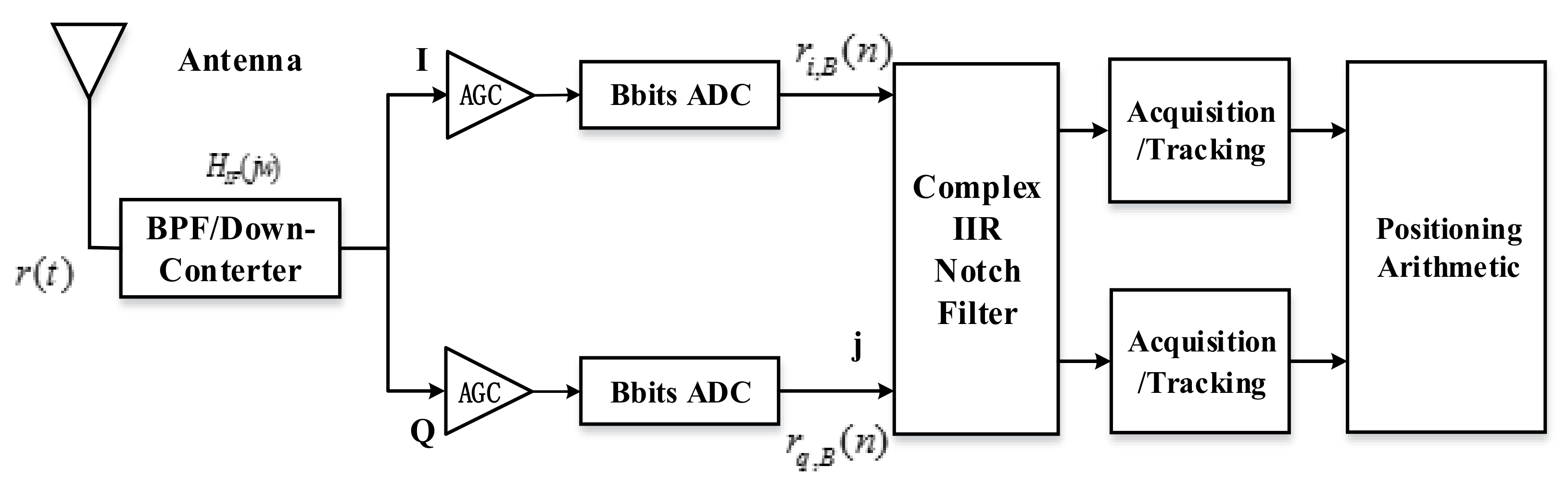
2.1. Signal Model
2.2. Distortion Analysis

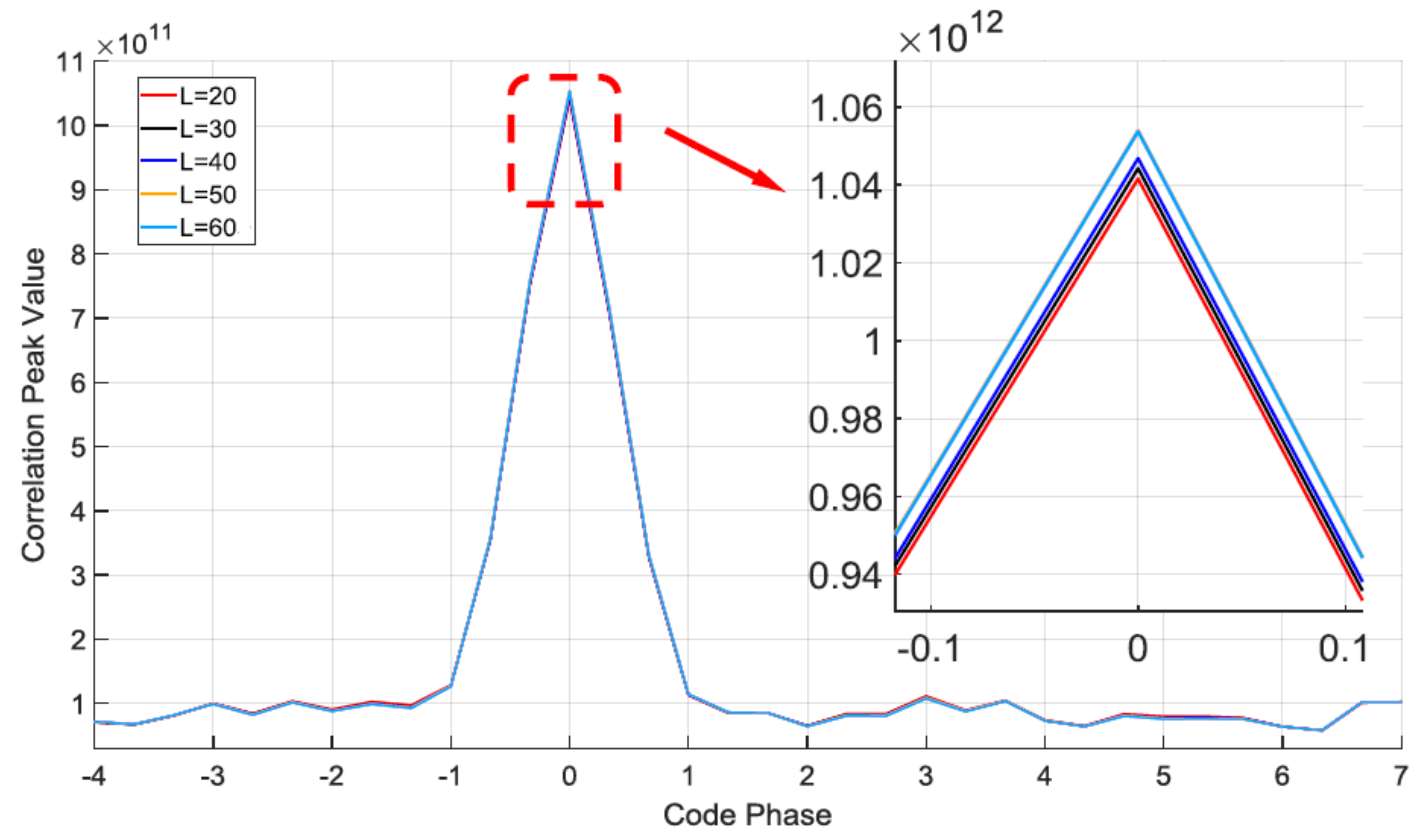
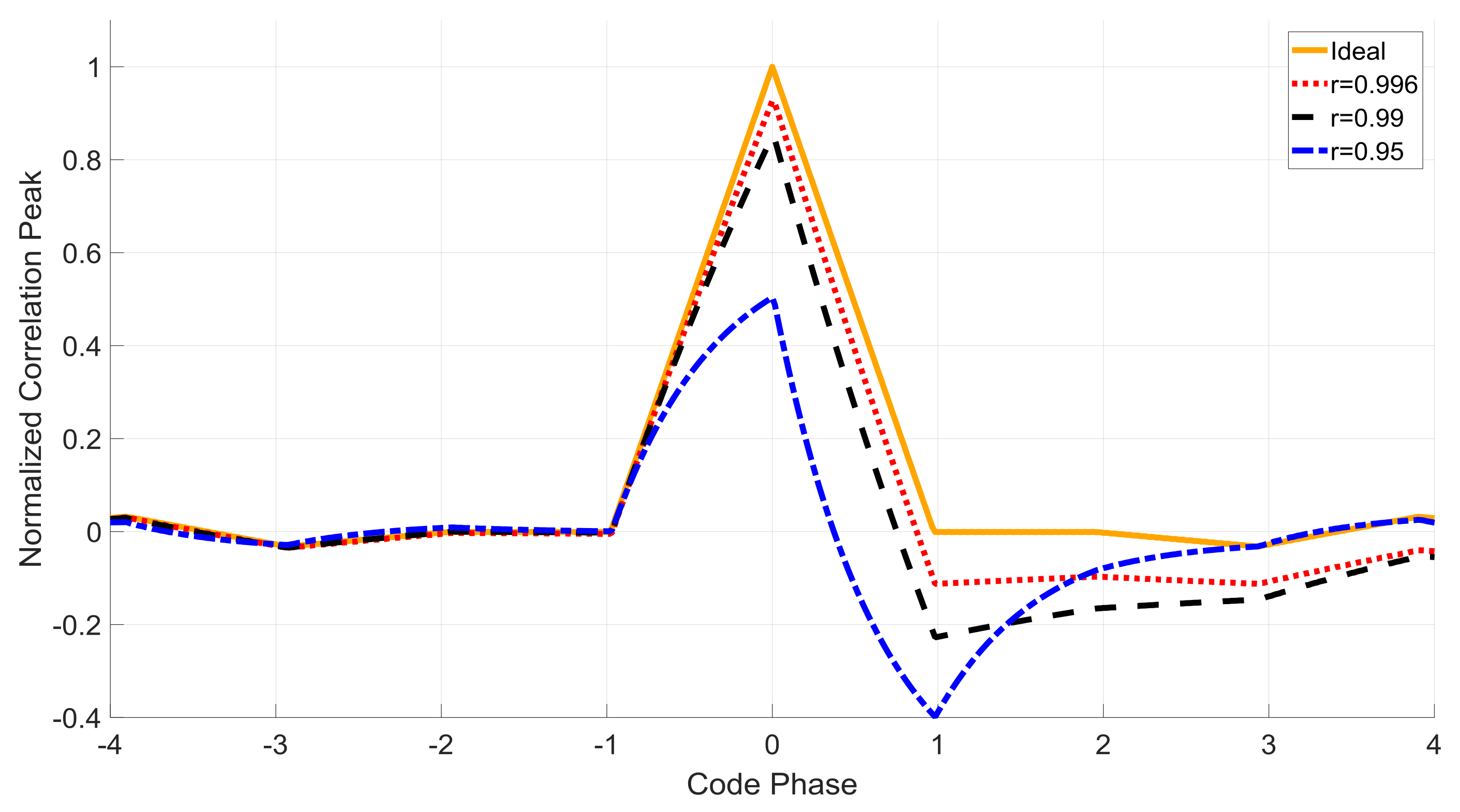
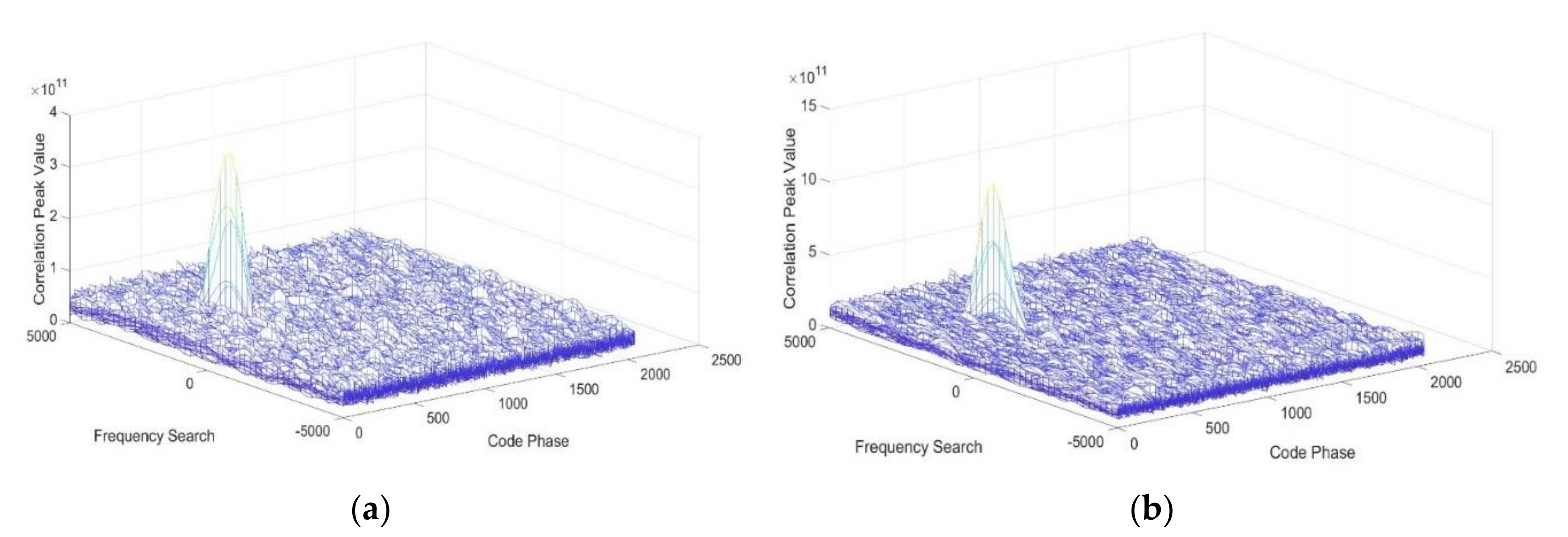
- After the interference suppression, the partial power in the notch bandwidth of navigation signals is lost, which causes the decline of the correlation peak value, yet without affecting the symmetry.
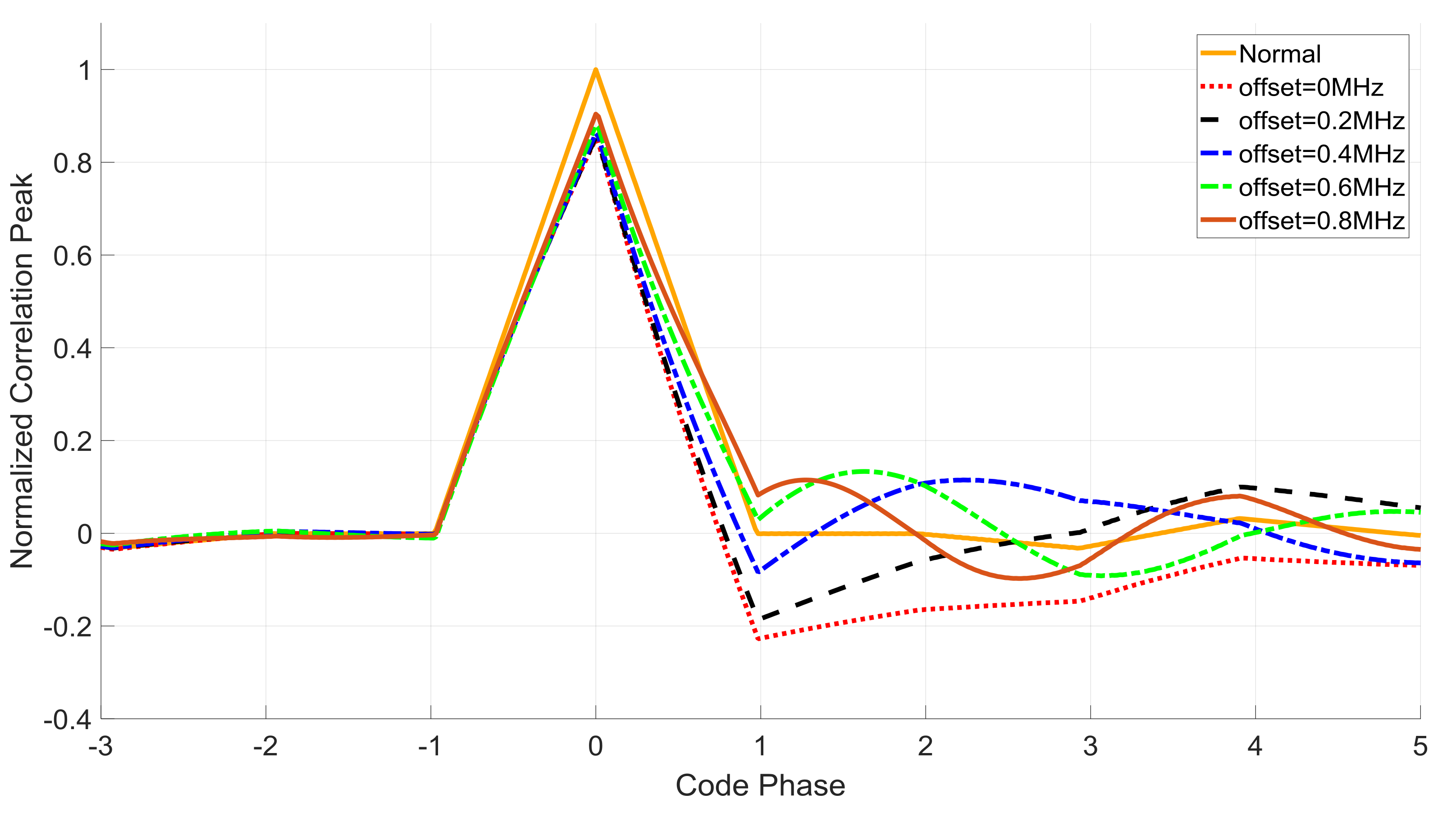
- From Equation (10), the nonlinear phase characteristic of IIR notch filters adds the ideal correlation peaks with the delayed correlation peaks together. And we can see the amplitude and phase distortion on the correlation results from Equation (5),
3. IIR Notch Filter Based on the Linear Phase Structure
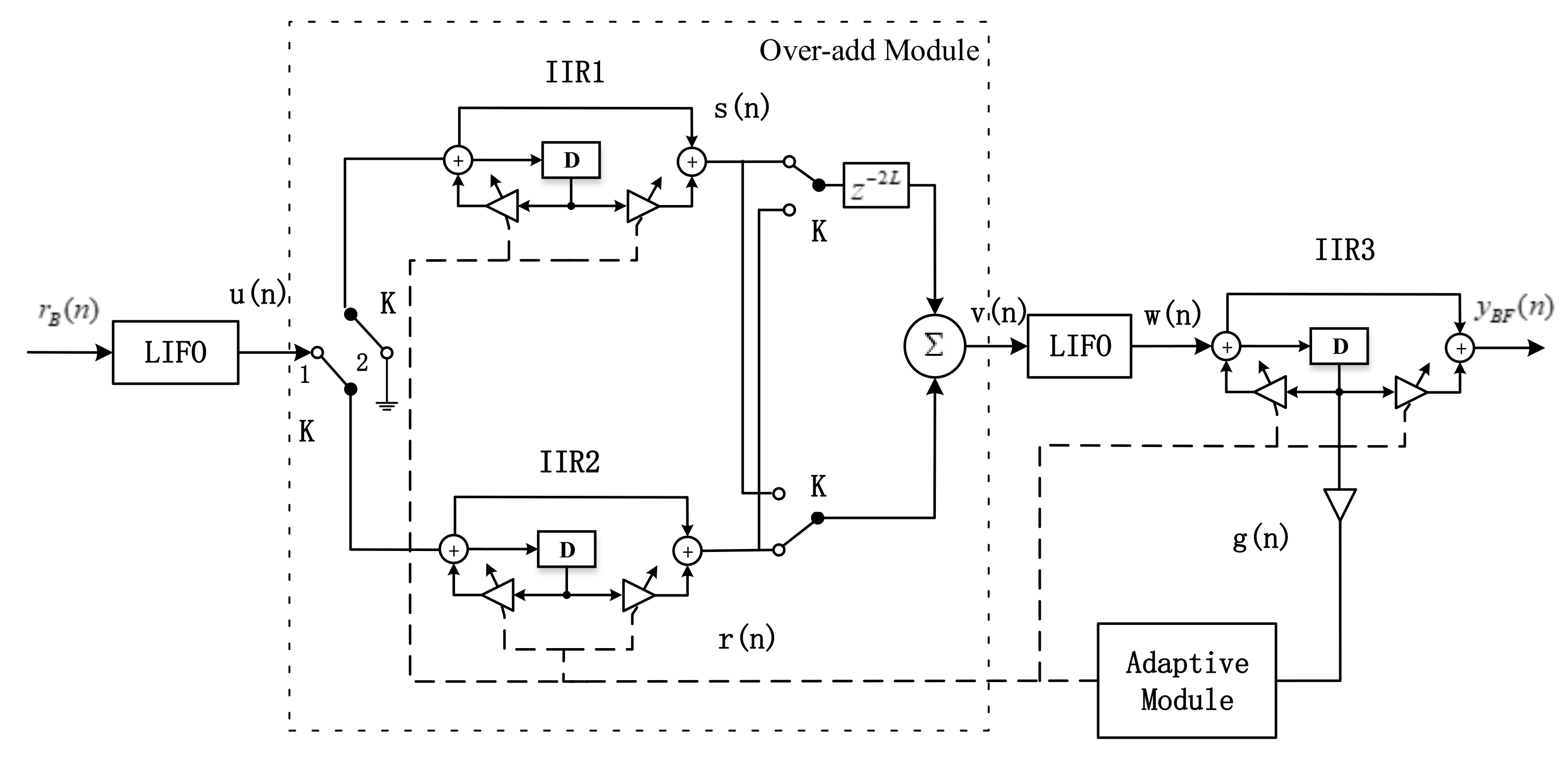
3.1. Linear Phase IIR Notch Filter Structure
- Step 1: The navigation signals enter the LIFO modules to make the signal time reversed, which indicates ;
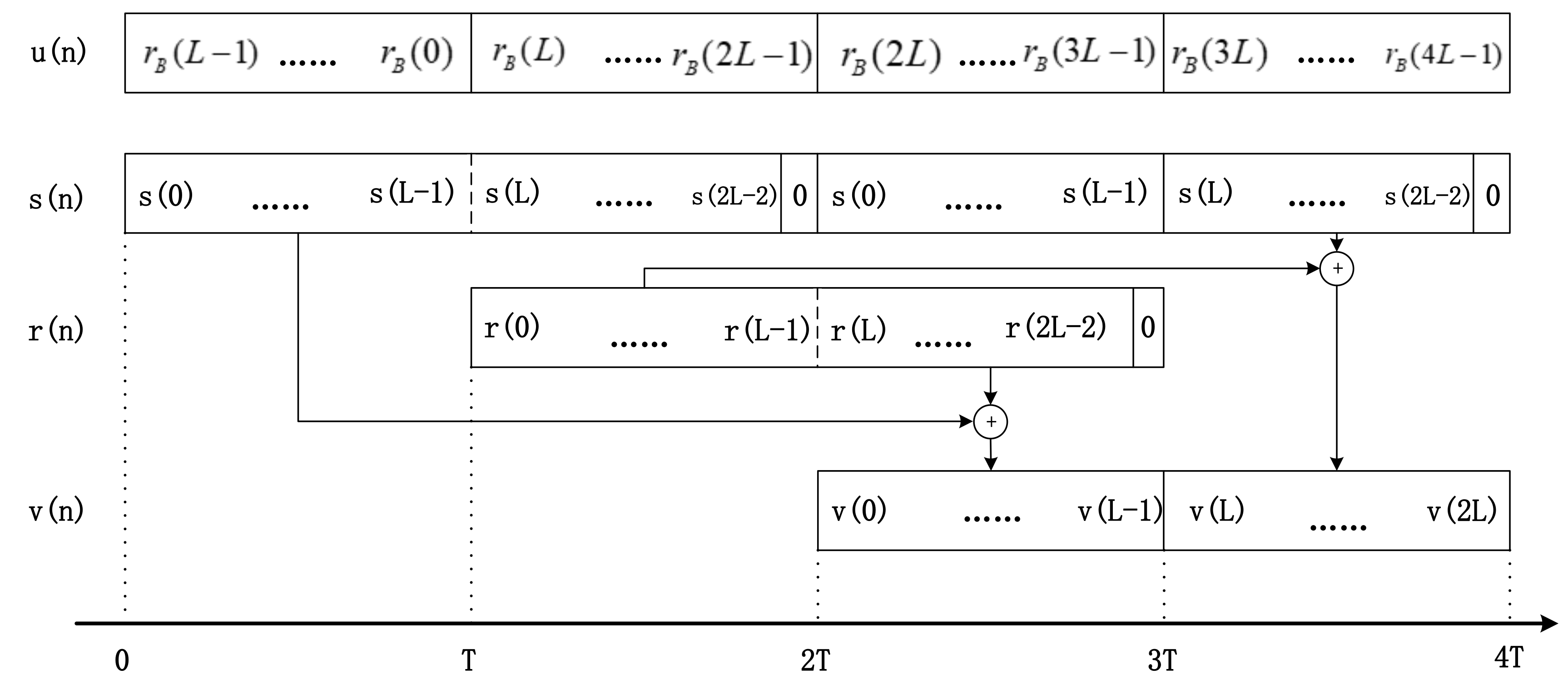
- Step 2: passes the overlap-add modules for sectioned convolution;
- Step 3: The signal passes the second LIFO modules. After that, the input signals are equivalent to pass a non-causal filter, whose unit impulse response is expressed as ;
- Step 4: The IIR3 outputs the final signals which is also the output of the linear phase IIR notch filter.
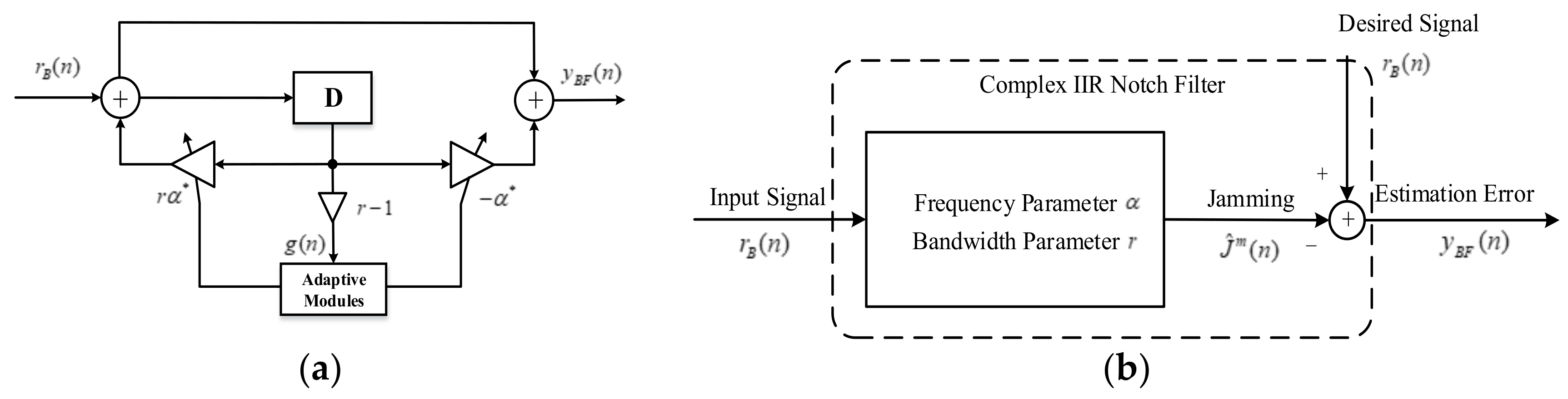
- Step 5: And consider the output signal and the adaptive signals of the last level notch filter as the adaptive modules input. It adjusts the notch frequency and −3 dB bandwidth parameters.
3.2. Corresponding Adaptive and Variable Step-Size Algorithm
3.3. Analysis of Filter Performance
4. Simulation and Verification
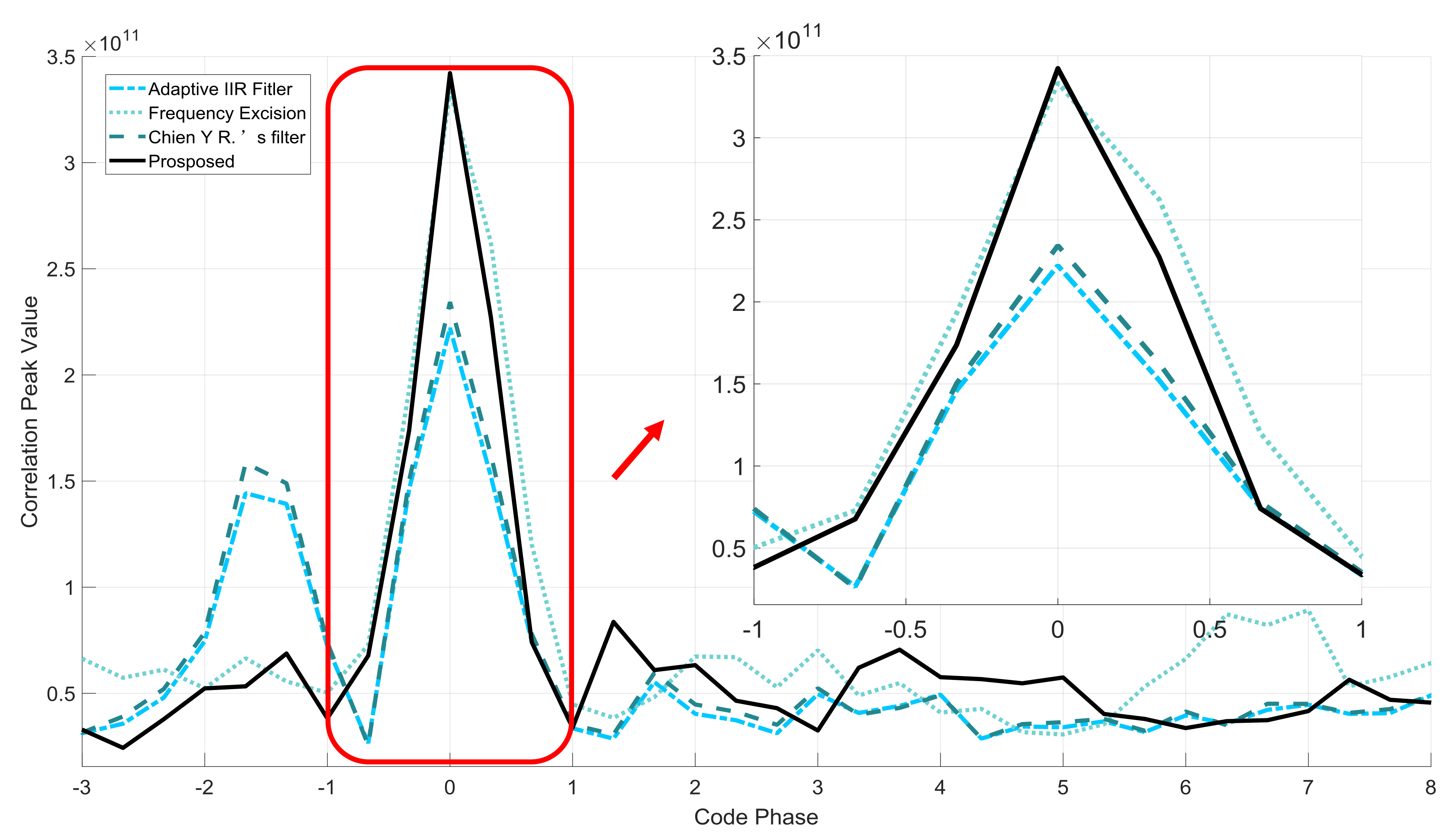
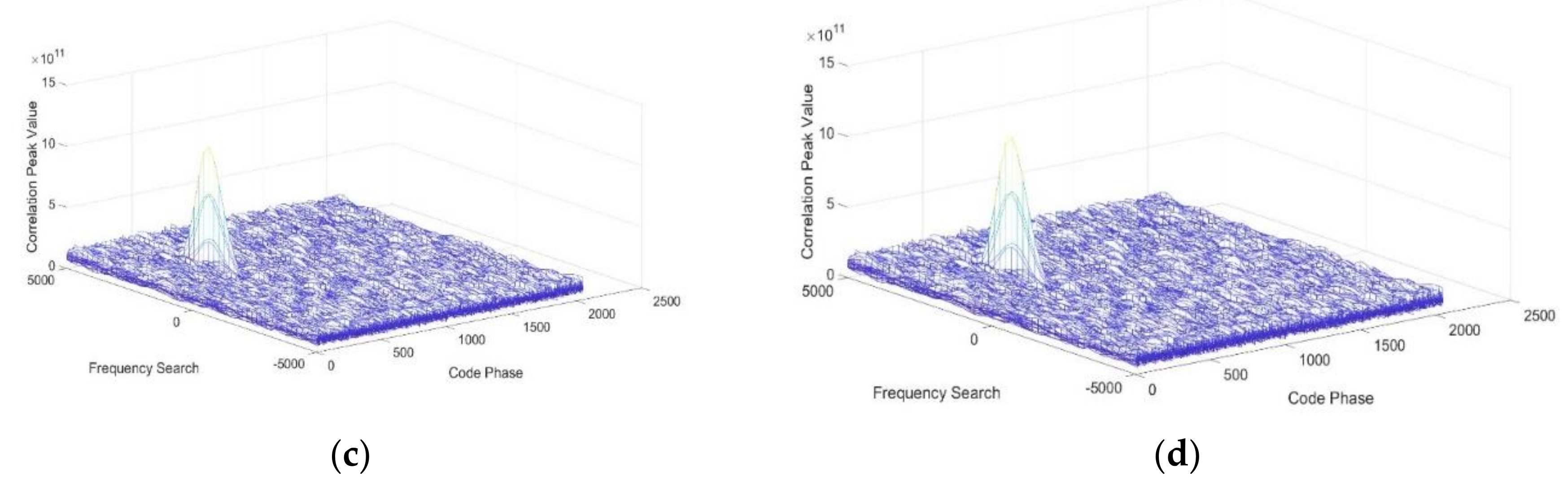
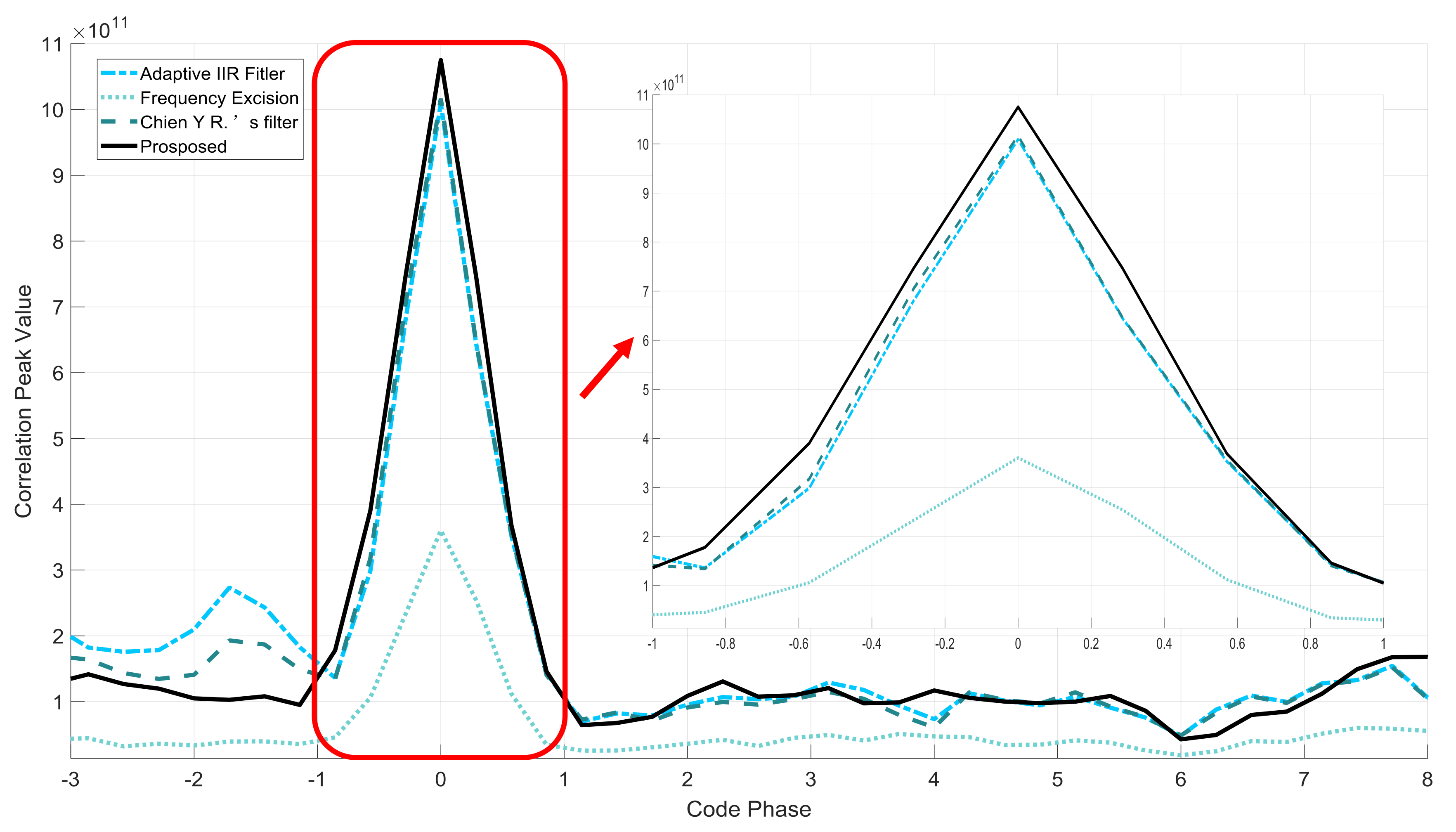
4.1. Comparison with Other Filters
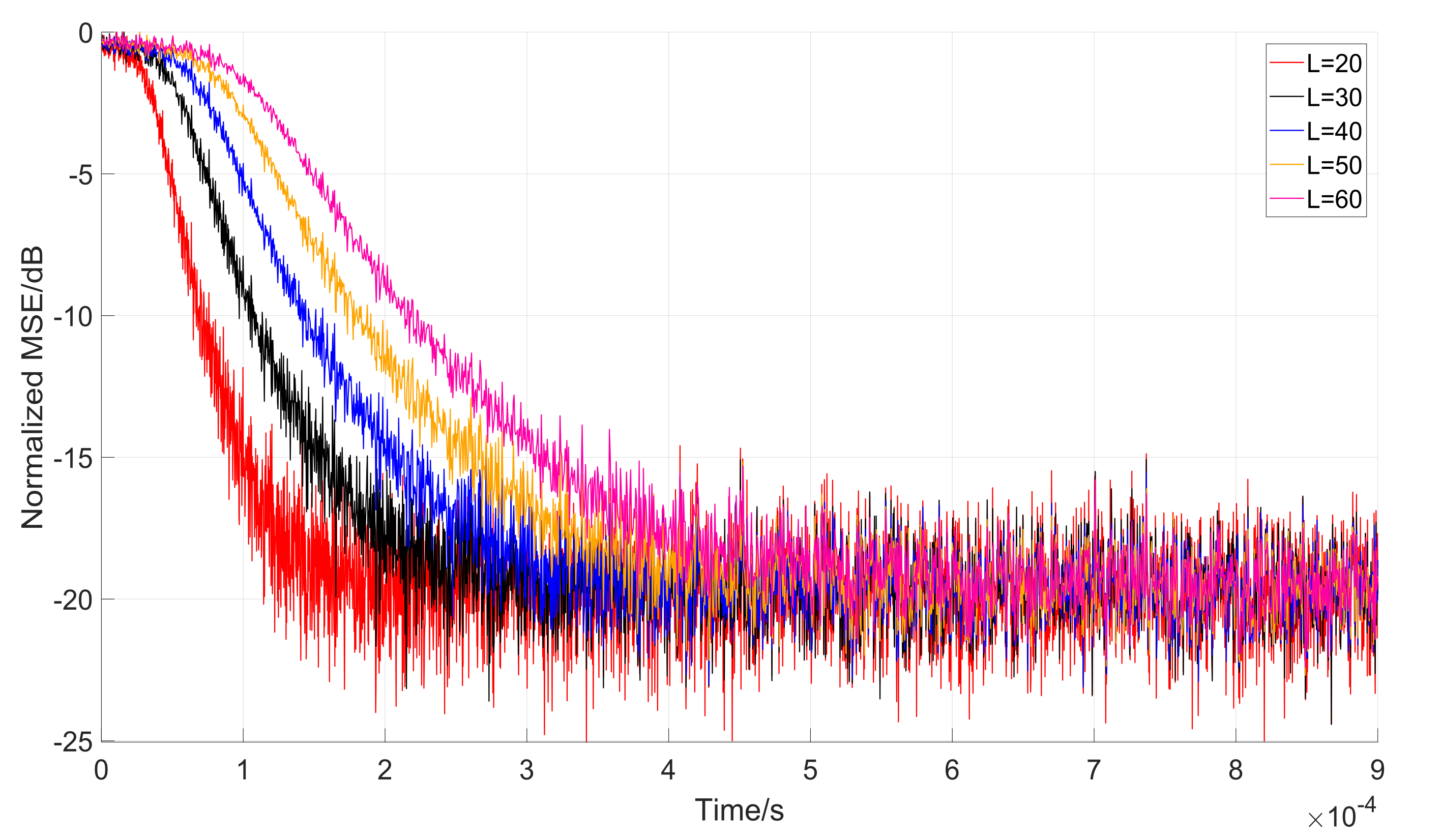
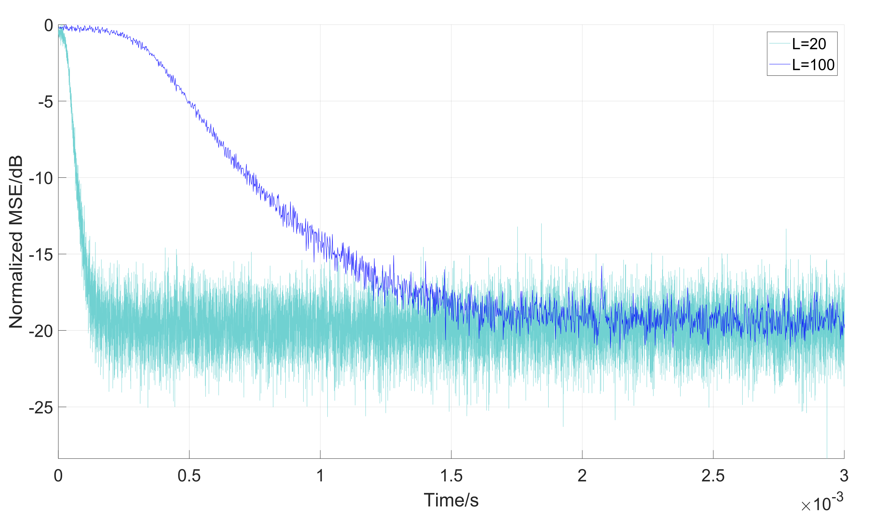
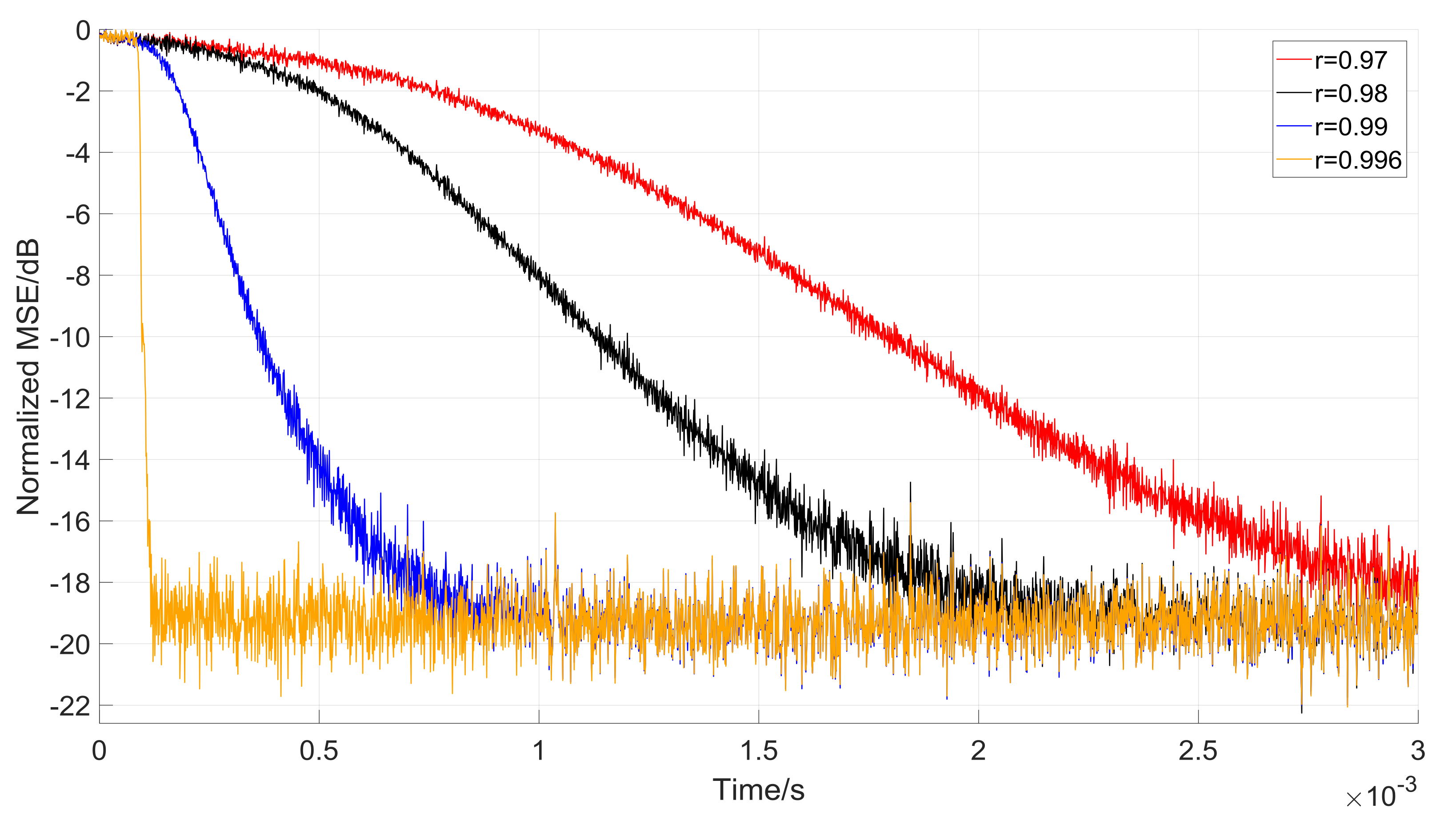
4.2. Anti-jamming Performance with Different Filter Parameters
5. Conclusions
Author Contributions
Acknowledgments
Conflicts of Interest
References
- Varshney, N.; Jain, R.C. An adaptive notch filter for narrow band interference removal. In Proceedings of the 2013 National Conference on Communications (NCC), New Delhi, India, 15–17 February 2013; pp. 1–5. [Google Scholar]
- Yan, X. A complex IIR adaptive notch filter and its application in QPSK spread spectrum communication. Signal Process. 2003, 19, 285–288. [Google Scholar]
- Nosan, A.; Punchalard, R. A Complex Adaptive Notch Filter Using Modified Gradient Algorithm; Elsevier North-Holland, Inc.: Amsterdam, The Netherlands, 2012. [Google Scholar]
- Betz, J.W. Effect of Narrowband Interference on GPS Code Tracking Accuracy. In Proceedings of the National Technical Meeting of the Institute of Navigation, Anaheim, CA, USA, 26–28 January 2000; pp. 16–27. [Google Scholar]
- Chien, Y.R.; Chen, P.Y.; Fang, S.H. Novel Anti-Jamming Algorithm for GNSS Receivers Using Wavelet-Packet-Transform-Based Adaptive Predictors. Ieice Trans. Fundam. Electron. Commun. Comput. Sci. 2017, E100-, 602–610. [Google Scholar] [CrossRef]
- Savasta, S.; Presti, L.L.; Rao, M. Interference Mitigation in GNSS Receivers by a Time-Frequency Approach. IEEE Trans. Aerosp. Electron. Syst. 2013, 49, 415–438. [Google Scholar] [CrossRef]
- Rezaei, M.J.; Abedi, M.; Mosavi, M.R. New gps anti-jamming system based on multiple short-time fourier transform. Iet Radar Sonar Navig. 2016, 10, 807–815. [Google Scholar] [CrossRef]
- Daneshmand, S.; Jahromi, A.J.; Broumandan, A.; Lachapelle, G. GNSS space-time interference mitigation and attitude determination in the presence of interference signals. Sensors 2015, 15, 12180–12204. [Google Scholar] [CrossRef] [PubMed]
- Xu, H.; Cui, X.; Lu, M. An SDR-Based Real-Time Testbed for GNSS Adaptive Array Anti-Jamming Algorithms Accelerated by GPU. Sensors 2016, 16, 356. [Google Scholar] [CrossRef] [PubMed]
- Daneshmand, S.; Marathe, T.; Lachapelle, G. Millimetre Level Accuracy GNSS Positioning with the Blind Adaptive Beamforming Method in Interference Environments. Sensors 2016, 16, 1824. [Google Scholar] [CrossRef] [PubMed]
- Mao, W.L.; Ma, W.J.; Chien, Y.R.; Ku, C.H. New Adaptive All-pass Based Notch Filter for Narrowband/FM Anti-jamming GPS Receivers. Circuits Syst. Signal Process. 2011, 30, 527–542. [Google Scholar] [CrossRef]
- Li, X.; Wang, Y.; Chen, J. Time Delay Compensation of IIR Notch Filter for CW Interference Suppression in GNSS. In Proceedings of the 2013 IEEE 11th International Conference on Electronic Measurement & Instruments (ICEMI), Harbin, China, 16–19 August 2013; Volume 1, pp. 106–109. [Google Scholar]
- Li, Z.; Wang, F. The influence of the adaptive narrowband interference suppression filter on the acquisition performance of PN code. Chin. J. Electron. 2002, 30, 1768–1771. [Google Scholar]
- Chien, Y.R. Design of GPS Anti-Jamming Systems Using Adaptive Notch Filters. IEEE Syst. J. 2015, 9, 451–460. [Google Scholar] [CrossRef]
- Powell, S.R.; Chau, P.M. A technique for realizing linear phase IIR filters. IEEE Trans. Signal Process. 1991, 39, 2425–2435. [Google Scholar] [CrossRef]
- Stančić, G.; Nikolić, S. Digital linear phase notch filter design based on IIR all-pass filter application. Digit. Signal Process. 2013, 23, 1065–1069. [Google Scholar] [CrossRef]
- Nikolić, S.; Stančić, G. Design of IIR Notch Filter with Approximately Linear Phase. Circuits Syst. Signal Process. 2012, 31, 2119–2131. [Google Scholar] [CrossRef]
- Haykin, S. Adaptive Filter Theory, 3rd ed.; Prentice-Hall, Inc.: Upper Saddle River, NJ, USA, 1996. [Google Scholar]
- Phelts, R.E. Multicorrelator Techniques for Robust Mitigation of Threats to GPS Signal Quality; Stanford University: Stanford, CA, USA, 2001. [Google Scholar]
- Xie, G. Principles of GPS and Receiver Design; Publishing House of Electronics Industry: Beijing, China, 2009; Volume 7, pp. 61–63. [Google Scholar]
- Fu, J.J.; Zuo, Q.; Peng, Y. Realization of GPS Signals FFT Adaptive Anti-jamming Algorithm on FPGA. Navig. Position. Timing 2016, 5, 60–65. [Google Scholar]


| Navigation System | BDS B1 | |
|---|---|---|
| Sample Rate | 100 MHz | |
| Intermediate Frequency | 40.098 MHz | |
| Interference | 40.098 MHz CWI | 40.098 MHz NBI with 10 KHz bandwidth |
| Interference Power | −75 dBm | |
| Anti-Jamming Methods | CWI | NBI | ||||
|---|---|---|---|---|---|---|
| Correlation Peak Value | ∆ Ratio Test | /Chip | Correlation Peak Value | ∆ Ratio Test | /Chip | |
| Frequency Excision | 3.518 × 10¹¹ | 0.0119 | 0.06 | 3.422 × 10¹¹ | 0.0708 | 0.0354 |
| Adaptive IIR notch filter | 1.009 × 10¹² | 0.0227 | 0.0113 | 2.221 × 10¹¹ | 0.2736 | 0.1368 |
| Chien’s filter | 1.017 × 10¹² | 0.0295 | 0.015 | 2.343 × 10¹¹ | 0.2947 | 0.1474 |
| Proposed | 1.075 × 10¹² | 0.0005 | 0.00025 | 3.335 × 10¹¹ | 0.0093 | 0.0046 |
© 2018 by the authors. Licensee MDPI, Basel, Switzerland. This article is an open access article distributed under the terms and conditions of the Creative Commons Attribution (CC BY) license (http://creativecommons.org/licenses/by/4.0/).
Share and Cite
Zhao, H.; Hu, Y.; Sun, H.; Feng, W. A BDS Interference Suppression Technique Based on Linear Phase Adaptive IIR Notch Filters. Sensors 2018, 18, 1515. https://doi.org/10.3390/s18051515
Zhao H, Hu Y, Sun H, Feng W. A BDS Interference Suppression Technique Based on Linear Phase Adaptive IIR Notch Filters. Sensors. 2018; 18(5):1515. https://doi.org/10.3390/s18051515
Chicago/Turabian StyleZhao, Hongbo, Yinan Hu, Hua Sun, and Wenquan Feng. 2018. "A BDS Interference Suppression Technique Based on Linear Phase Adaptive IIR Notch Filters" Sensors 18, no. 5: 1515. https://doi.org/10.3390/s18051515
APA StyleZhao, H., Hu, Y., Sun, H., & Feng, W. (2018). A BDS Interference Suppression Technique Based on Linear Phase Adaptive IIR Notch Filters. Sensors, 18(5), 1515. https://doi.org/10.3390/s18051515