Abstract
Dempster–Shafer evidence theory is widely applied in various fields related to information fusion. However, how to avoid the counter-intuitive results is an open issue when combining highly conflicting pieces of evidence. In order to handle such a problem, a weighted combination method for conflicting pieces of evidence in multi-sensor data fusion is proposed by considering both the interplay between the pieces of evidence and the impacts of the pieces of evidence themselves. First, the degree of credibility of the evidence is determined on the basis of the modified cosine similarity measure of basic probability assignment. Then, the degree of credibility of the evidence is adjusted by leveraging the belief entropy function to measure the information volume of the evidence. Finally, the final weight of each piece of evidence generated from the above steps is obtained and adopted to modify the bodies of evidence before using Dempster’s combination rule. A numerical example is provided to illustrate that the proposed method is reasonable and efficient in handling the conflicting pieces of evidence. In addition, applications in data classification and motor rotor fault diagnosis validate the practicability of the proposed method with better accuracy.
1. Introduction
Multi-sensor data fusion technology has received significant attention in a variety of fields, as it combines the collected information from multi-sensors, which can enhance the robustness and safety of a system. In wireless sensor networks applications, however, the data that are collected from the sensors are often imprecise and uncertain [1]. How to model and handle the uncertainty information is still an open issue. To address this problem, many mathematical approaches have been presented, such as the fuzzy sets theory [2,3], that focuses on the intuitive reasoning by taking into account human subjectivity and imprecision; the intuitionistic fuzzy sets theory [4] which generalizes fuzzy sets by considering the uncertainty in the assignment of membership degree known as the hesitation degree; evidence theory [5,6,7], as a general framework for reasoning with uncertainty, with understood connections to other frameworks such as probability, possibility, and imprecise probability theories; rough sets theory [8,9] where its methodology is concerned with the classification and analysis of imprecise, uncertain, or incomplete information and knowledge, which is considered one of the first non-statistical approaches in data analysis; evidential reasoning [10,11] which is a generic evidence-based multi-criteria decision analysis (MCDA) approach for dealing with problems having both quantitative and qualitative criteria under various uncertainties including ignorance and randomness; Z numbers [12,13], that intend to provide a basis for computation with numbers which are not totally reliable; D numbers theory [14,15,16,17] which is a generalization of Dempster–Shafer theory, but does not follow the commutative law; and so on [18,19,20,21]. In addition, mixed intelligent methods have been applied in decision making [22], risk analysis [23], supplier selection [24], pattern recognition [25], classification [26], human reliability analysis [27], and fault diagnosis [28], etc. In this paper, we focus on evidence theory to deal with the uncertain problem of multi-sensor data fusion.
Dempster–Shafer evidence theory was firstly presented by Dempster [5] in 1967; later, it was extended by Shafer [6] in 1976. Dempster–Shafer evidence theory is effective to model both of the uncertainty and imprecision without prior information, so it is widely applied in various fields for information fusion [29,30,31,32]. Nevertheless, it may result in counter-intuitive results when combining highly conflicting pieces of evidence [33]. To address this issue, many methods have been presented in recent years [34,35,36]. On the one hand, some researchers focused on amending Dempster’s combination rule. On the other hand, some researchers tried to pretreat the bodies of evidence before using Dempster’s combination rule. In terms of of amending Dempster’s combination rule, the major works contain Smets’s unnormalized combination rule [37], Dubois and Prade’s disjunctive combination rule [38], and Yager’s combination rule [39]. However, the modification of combination rule often breaks the good properties, like commutativity and associativity. Furthermore, if the sensor failure gives rise to the counter-intuitive results, the modification of combination rule is considered to be unreasonable. Therefore, in order to resolve the fusion problem of highly conflicting pieces of evidence, researchers prefer to pretreat the bodies of evidence. With respect to pretreating the bodies of evidence, the main works contain Murphy’s simple average approach of the bodies of evidence [40], and Deng et al.’s weighted average of the masses based on distance of evidence [41]. Deng et al.’s method [41] conquered the deficiency of the method in [40]. However, the impact of evidence itself was neglected in the decision-making process.
Hence, in this paper, a weighted combination method for conflicting pieces of evidence in multi-sensor data fusion is proposed to resolve fusion problem of highly conflicting evidence. First, the credibility degree of each piece of evidence is determined on the basis of the modified cosine similarity measure of basic probability assignment [42]. Then, credibility degree of each piece of evidence is modified by adopting the belief entropy function [43] to measure the information volume of the evidence. Finally, the modified credibility degree of each piece of evidence is used to adjust its corresponding body of evidence to obtain the weighted averaging evidence before using Dempster’s combination rule. A numerical example is given to illustrate the feasibility and effectiveness of the proposed method. Additionally, the proposed method is applied in data classification and motor rotor fault diagnosis, which validates the practicability of it.
The rest of this paper is organized as follows. Section 2 briefly introduces the preliminaries of this paper. After that, Section 3 proposes the novel method, which is based on the similarity measure of evidence and belief function entropy. Then, Section 4 gives a numerical example to show the effectiveness of the proposed method. A statistical experiment is carried out in Section 5. Afterwards, the proposed method is applied to data set classification, and motor rotor fault diagnosis is performed in Section 6. Finally, Section 7 gives the conclusions.
2. Preliminaries
2.1. Data Fusion
Data fusion can be identified as a combination of multiple sources to obtain improved information with less expensive, higher quality, or more relevant information [44]. General data fusion structure can be classified into three types based on the different stages: data-level, feature-level, and decision-level, as referred in [45].
In the data-level fusion, all raw data from sensors for a measured object are combined directly. Then, a feature vector is extracted from the fused data. Fusion of data at this level consists of the maximum information so that it can generate good results. However, sensors used in the data-level fusion, such as the sensors reporting vibration signals, must be homogeneous. As a consequence, the data-level fusion is limited in the actual application environment, because many physical quantities can be measured for a more comprehensive analysis. In the feature-level fusion, heterogeneous sensors can be used to report the data. According to the types of collected raw data, the features are extracted from the sensors. Then, these heterogeneous sensor data are combined at the feature-level stage. All of the feature vectors are combined into a single feature vector, which is then utilized in a special classification model for decision-making. In the decision-level fusion, the processes of feature extraction and pattern recognition are sequentially conducted for the data collected from each sensor. Then, the produced decision vectors are combined by using decision-level fusion techniques such as the Bayesian method, Dempster–Shafer evidence theory, or behavior knowledge space.
Because of the advantages of multi-sensor data fusion technology, it has been widely applied in various fields, such as in fault diagnosis [46,47,48], target tracking [49,50], health care analysis [51,52], image processing [53], attack detection [54], estimation of ship dynamics [55], and characterization of built environments [56].
In this paper, we focus on decision-level fusion, and try to improve the performance of the system based on Dempster–Shafer evidence theory.
2.2. Dempster-Shafer Evidence Theory
Dempster–Shafer evidence theory was firstly proposed by Dempster [5] and was then further developed by Shafer [6]. Dempster–Shafer evidence theory, as a generalization of Bayesian inference, asks for weaker conditions, which makes it more flexible and effective to model both the uncertainty and imprecision. The basic concepts are introduced as below.
Definition 1.
Let U be a set of mutually exclusive and collectively exhaustive events, indicated by
The set U is called frame of discernment. The power set of U is indicated by , where
and ∅ is an empty set. If , A is called a proposition or hypothesis.
Definition 2.
For a frame of discernment U, a mass function is a mapping m from to [0, 1], formally defined by
which satisfies the following condition:
In Dempster–Shafer evidence theory, a mass function can be also called as a basic probability assignment (BPA). If is greater than 0, A will be called as a focal element, and the union of all of the focal elements is known as the core of the mass function.
Definition 3.
For a proposition , the belief function is defined as
The plausibility function is defined as
where .
Apparently, is equal or greater than , where the function is the lower limit function of proposition A and the function is the upper limit function of proposition A.
Definition 4.
Let the two BPAs be and on the frame of discernment U. Assuming that these BPAs are independent, Dempster’s rule of combination, denoted by , known as the orthogonal sum, is defined as below:
with
where B and D are also the elements of , and K is a constant that presents the conflict between the two BPAs.
Note that Dempster’s combination rule is only practicable for the two BPAs with the condition .
2.3. Modified Cosine Similarity Measure of BPAs
A modified cosine similarity measure is proposed by Jiang [42]. Because it considers three important factors, namely, angle, distance, and vector norm, the modified cosine similarity measure is an efficient approach to measure the similarity between vectors more precisely. The modified cosine similarity measure among the BPAs can determine whether the pieces of evidence conflict with each other. A large similarity indicates that this piece of evidence has more support from another piece of evidence, while a small similarity indicates that this piece of evidence has less support from another piece of evidence.
Definition 5.
Let and be two vectors of . The modified cosine similarity between vectors E and F is defined as
where α is a constant whose value is greater than 1, P is the Euclidean distance between the two vectors E and F, is the distance-based similarity measure, is the minimum of and , and is the cosine similarity. The larger the α is, the greater the distance impact on vector similarity will be.
Definition 6.
Let and be the BPAs in the frame of discernment . The two vectors are expressed as
Then, the belief function vector similarity and the plausibility function vector similarity can be calculated. The new similarity of BPAs is defined as
with
where λ is the total uncertainty of BPAs, which is defined as
Because and , if , then . Otherwise, if , then . The larger the uncertainty is, the greater the influence on the similarity of BPA will be.
2.4. Belief Entropy
A novel type of belief entropy, known as the Deng entropy, was first proposed by Deng [43]. When the uncertain information is expressed by probability, the Deng entropy degenerates to the Shannon entropy. Hence, the Deng entropy is regarded as a generalization of the Shannon entropy. It is an efficient mathematical tool to measure the uncertain information, especially when the uncertain information is expressed by the BPA. Because of its advantage in measuring the uncertain information, the Deng entropy is applied in a variety of areas [57,58]. The basic concepts are introduced below.
Definition 7.
Let B be a hypothesis or proposition of the BPA m in the frame of discernment U and be the cardinality of B. The Deng entropy of the BPA m is defined as follows:
When the belief value is only allocated to the singleton, the Deng entropy degenerates to the Shannon entropy, i.e.,
The larger the value of the cardinality of the hypothesis or proposition, the larger the value the Deng entropy of evidence, which means that the piece of evidence involves more information. Therefore, if a piece of evidence has a large Deng entropy value, it has more support from other pieces of evidence, indicating that this piece of evidence plays an important role in the evidence combination.
3. The Proposed Method
In this paper, a weighted combination method for conflicting pieces of evidence multi-sensor data fusion is proposed by combining the modified cosine similarity measure of evidence with the belief entropy function. In contrast to the method of Jiang et al. [42], in the proposed method, the impact of evidence itself is considered in the process of fusion of multiple pieces of evidence by leveraging the belief entropy [43], i.e., a useful uncertainty measure tool, to measure the information volume of each piece of evidence, so that the proposed method can combine multiple pieces of evidence with greater accuracy. This will be discussed further in the next section.
3.1. Process Steps
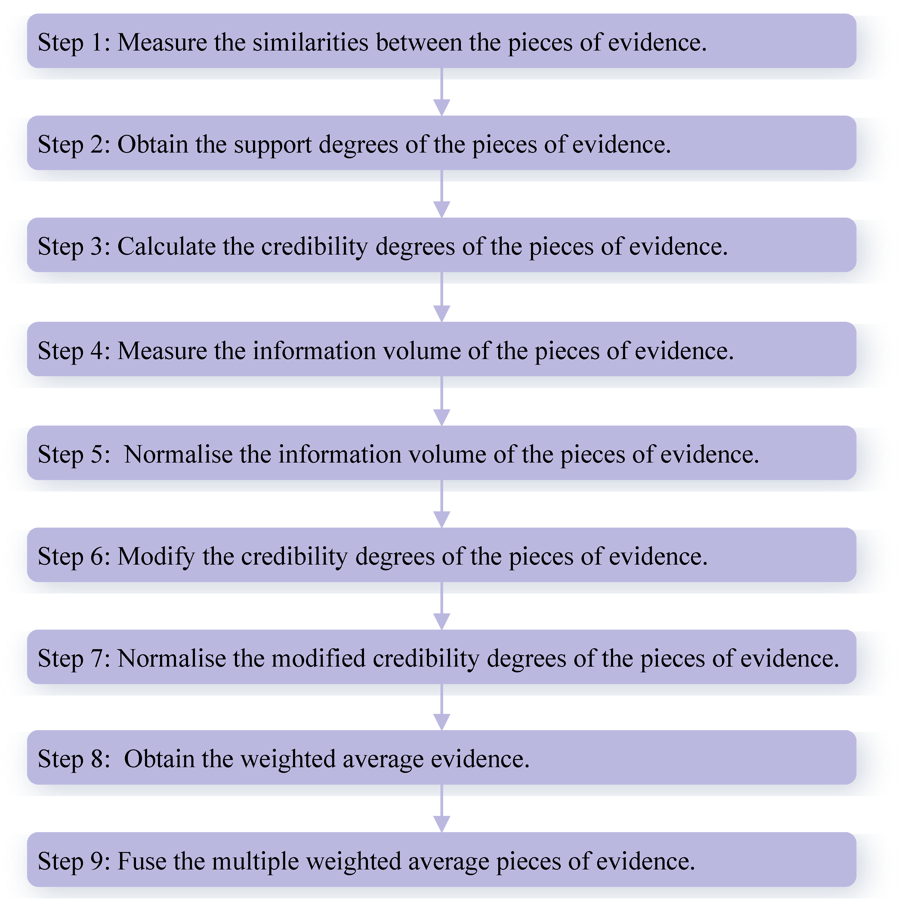
The proposed method is composed of the following procedures. The credibility degree of the pieces of evidence is first determined on the basis of the similarity measure among the BPAs. Then, the credibility degree is modified by leveraging the belief entropy function to measure the information volume of the evidence. Afterwards, the final weight of each piece of evidence is obtained and adopted to adjust the body of evidence before using Dempster’s combination rule. The specific calculation processes are listed as follows. The flowchart of the proposed method is shown in Figure 1.
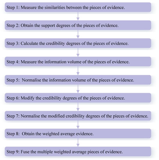
Figure 1.
The flowchart of the proposed method.
Step 1: Measure the similarities between the pieces of evidence.
The similarity measure between the BPAs and can be obtained by Equations (11)–(13). Then, a similarity measure matrix (SMM) can be constructed as follows:
Step 2: Obtain the support degrees of the pieces of evidence.
The support degree of the BPA ), denoted as , is defined as follows:
Step 3: Calculate the credibility degrees of the pieces of evidence.
The credibility degree of the BPA ), denoted as , is defined as follows:
Step 4: Measure the information volume of the pieces of evidence.
According to Equation (14), the belief entropy of the BPA ) can be calculated. To avoid assigning zero weight to the evidence, the information volume is used for measuring the uncertain information of . It is defined as follows:
Step 5: Normalize the information volume of the pieces of evidence.
The information volume of the BPA ) will be normalized as below:
Step 6: Modify the credibility degrees of the pieces of evidence.
Based on the normalized information volume, the credibility degree of the BPA ) will be modified, denoted as :
Step 7: Normalize the modified credibility degrees of the pieces of evidence.
The modified credibility degree of the BPA ) will be normalized as below, and is considered as the final weight to adjust the bodies of evidence.
Step 8: Obtain the weighted average evidence.
Based on the modified credibility degree of the BPA ), the weighted average evidence is defined as follows:
Step 9: Fuse multiple weighted average pieces of evidence.
When k number of pieces of evidence exist, the weighted average evidence will be fused through Dempster’s combination rule Equation (7) via times as below,
Ultimately, we can obtain the final fusion result of the evidence.
3.2. Algorithm
Let be a set of multiple pieces of evidence. After receiving k pieces of evidence, a fusion result is expected to be generated for decision-making support. The weighted fusion method for multiple pieces of evidence is outlined in Algorithm 1.
As shown in Algorithm 1, it provides a formal expression in terms of the specific calculation processes of the proposed method listed in Section 3.1. To be specific, Lines 2–7 explain how to measure the similarities between the pieces of evidence and construct the similarity measure matrix for k pieces of evidence. Lines 9–11 show how to obtain the support degrees for k pieces of evidence. Lines 13–15 represent how to calculate the credibility degrees for k pieces of evidence. Lines 17–19 explain how to measure the information volumes for k pieces of evidence. Lines 21–23 express how to normalize the information volumes for k pieces of evidence. Lines 25–27 state how to modify the credibility degrees for k pieces of evidence. Lines 29–31 show how to normalize the modified credibility degrees for k pieces of evidence. Line 33 describes how to obtain the weighted average evidence based on k pieces of evidence. Lines 35–37 depict how to generate the fusion result.

4. Numerical Example
In this section, in order to demonstrate the feasibility and effectiveness of the proposed method, a numerical example is illustrated.
Example 1.

Consider the decision-making problem of the multi-sensor-based target recognition system from [59] associated with five different kinds of sensors to observe objects, where . Here, a, b, and c are the three objects in the frame of discernment U. The five BPAs that are collected by the system are listed as shown in Table 1.
Table 1.
The basic probability assignments (BPAs) for the example.
- Step 1:
- The similarity measure between the BPAs and can be constructed as below:
- Step 2:
- The support degree of the BPA is calculated as shown in Table 2.
Table 2. The calculated results in terms of support degree, credibility degree, information volume, normalized information volume, credibility degree, and modified credibility degree of BPAs.
- Step 3:
- The credibility degree of the BPA is obtained as shown in Table 2.
- Step 4:
- The information volume of the BPA is measured as shown in Table 2.
- Step 5:
- The information volume of the BPA is normalized as shown in Table 2, denoted by .
- Step 6:
- The credibility degree of the BPA is modified as shown in Table 2.
- Step 7:
- The modified credibility degree of the BPA is normalized as shown in Table 2.
- Step 8:
- The weighted average evidence is computed as shown in Table 3.
Table 3. The weighted average evidence (WAE(m)) and final fusion result (Fus(m)).
- Step 9:
- By fusing the weighted average evidence via Dempster’s combination rule four times, the final fusion result of evidence can be produced as shown in Table 3.
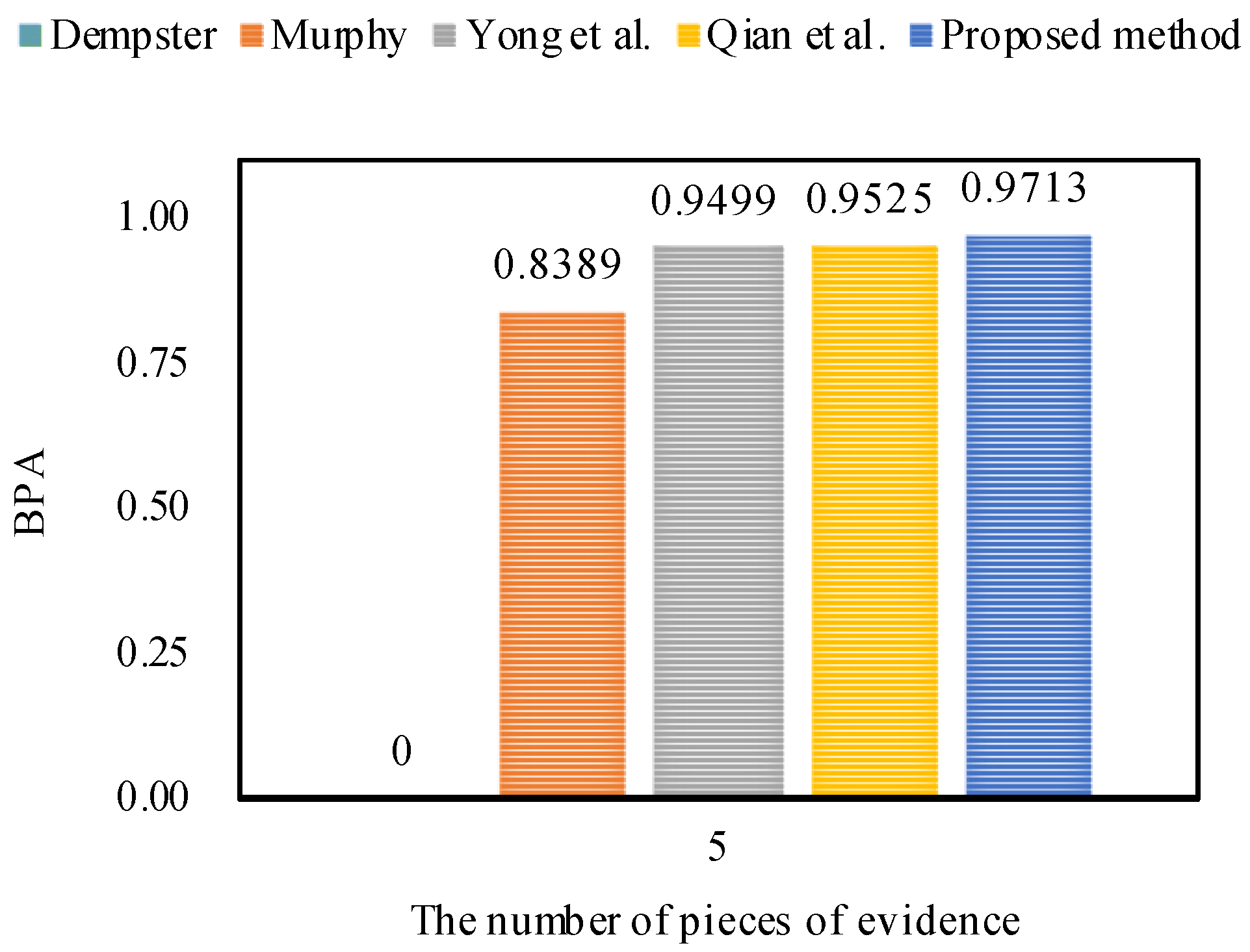
From Example 1, it is obvious that highly conflicts with other pieces of evidence. The fusing results that are obtained by different combination approaches are presented in Table 4. In addition, the comparisons of target a’s BPA in terms of different combination rules are shown in Figure 2.
Table 4.
Evidence fusion results based on different combination rules.
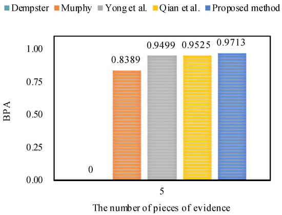
Figure 2.
The comparisons of target a’s BPA in terms of different methods.
As shown in Table 4, no matter how many pieces of evidence support target a, Dempster’s combination method [5] always generates a counterintuitive result. As the number of pieces of evidence increases to three, Murphy’s combination method [40] and Deng et al.’s combination method [41] cannot deal with the highly conflicting pieces of evidence very well, because the BPA values of object a generated by Murphy’s method [40] and Deng et al.’s method [41] are 33.24% and 44.77%, respectively, which are smaller than 50%. When the number of pieces of evidence increases from four to five, Murphy’s combination method [40] and Deng et al.’s combination method [41] work well, and the BPA values of object a generated by Murphy’s method [40] and Deng et al.’s method [41] increase up to 83.89% and 94.99%, respectively.
On the other hand, as shown in Table 4, Qian et al.’s combination method [59] and the proposed method show reasonable results and can efficiently deal with the highly conflicting pieces of evidence as the number of pieces of evidence increases from three to five. In the face of five pieces of evidence, the BPA value of object a generated by the proposed method increases to 97.13% which is much higher than for other combination approaches, as shown in Figure 2. Therefore, it is concluded that the proposed method is as feasible and effective as related approaches.
5. Statistical Experiment
In this section, in order to make a sound comparison, a statistical experiment is carried out with multiple pieces of initial data for the comparison of the proposed method with other related methods.
This statistical experiment is implemented based on Example 1. In the experimental setting, for generating multiple initial data 100 times, we provide a variation range [−0.1, 0.1] for each BPA of , and vary the values of BPAs of randomly.
Then, the generated multiple pieces of initial data are fused by utilizing the different methods, namely, Dempster’s combination method [5], Murphy’s combination method [40], Deng et al.’s combination method [41], Jiang et al.’s combination method [42], and the proposed method.
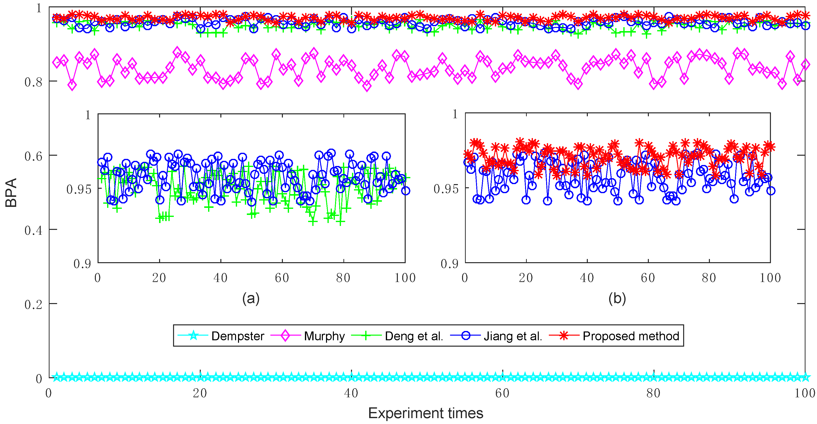
The experimental results of target a’s BPA generated by different combination methods are shown in Figure 3. From the comparison results, it is obvious that Murphy’s combination method [40], Deng et al.’s combination method [41], Jiang et al.’s combination method [42], and the proposed method are more efficient than Dempster’s combination method [5], because Dempster’s combination method cannot effectively deal with the conflicting pieces of evidence, and thus always generates counterintuitive results where target a’s BPA value is 0 (under 0.5). In contrast, the other methods can effectively cope with the conflicting evidence and recognize the target a, where its corresponding BPA value is always larger than 0.5 under multiple experiments. On the other hand, because Murphy’s combination method is a simply average-weighted approach to the bodies of evidence, its overall performance is poorer than that of Deng et al.’s combination method, Jiang et al.’s combination method, and the proposed method to a certain extent.

Figure 3.
The comparisons of target a’s BPAs obtained by different combination methods where the multiple BPAs are generated randomly 100 times. (a) The comparisons of Deng et al.’s combination method and Jiang et al.’s combination method; (b) The comparisons of Jiang et al.’s combination method and the proposed method.
Furthermore, as shown in Figure 3a, Jiang et al.’s combination method [42] which is based on the modified cosine similarity measure, is more effective than Deng et al.’s combination method [41] that is based on the Jousselme distance as a whole. This is the reason that the modified cosine similarity measure is considered in this study.
In order to improve the performance of Jiang et al.’s combination method, we investigate and find that in the process of fusion of multiple pieces of evidence, the impact of the evidence itself is overlooked in their method. Hence, we also take the belief entropy into consideration to measure the information volume of each piece of evidence in the course of fusion and design the proposed method. Consequently, as shown in Figure 3b, it can be noted that the proposed method is superior to Jiang et al.’s combination method [42] with a higher target a BPA value.
6. Applications
In this section, the proposed approach is applied to data set classification and motor rotor fault diagnosis, respectively, to validate its practicability, in which the experimental data in [48,59] are leveraged for the comparison among different approaches.
6.1. Data Set Classification
Consider the data set classification problem associated with a frame of discernment U consisting of three species of flowers given by U = , , = in terms of four numerical attributes of flowers given by , , , , where the BPAs of instances are modeled with noisy data and given in Table 5 from [59].
Table 5.
The BPAs of flower instances.
- Step 1:
- The similarity measure between the BPAs and can be constructed as below:
- Step 2:
- The support degree of the BPA is calculated as follows:
- Step 3:
- The credibility degree of the BPA is obtained as below:
- Step 4:
- The information volume of the BPA is measured as follows:
- Step 5:
- The information volume of the BPA is normalised as follows:
- Step 6:
- The credibility degree of the BPA is modified as below:
- Step 7:
- The modified credibility degree of the BPA is normalized as follows:
- Step 8:
- The weighted average evidence is computed as below:
- Step 9:
- By fusing the weighted average evidence via Dempster’s combination rule four times, the final fusion result of the evidence can be produced as follows:
The fusion results based on different combination approaches that were applied on the data set are presented in Table 6. From the experimental results, it can be seen that Dempster’s combination method [5] and Murphy’s combination method [40] always generate counterintuitive results and classify the species of flower as , even when the number of pieces of evidence increases from two () to four (). By contrast, Deng et al.’s combination method [41] works well when the number of pieces of evidence is increased up to four (), because it can classify the species of flower as the target with a belief value of 73.01%.
Table 6.
The comparison of different methods applied in the data set classification.
Obviously, Qian et al.’s combination method [59] and the proposed method show reasonable results and classify the species of flower as the target with 83.38% and 86.93% belief values, respectively. Therefore, we can conclude that the proposed method is more efficient than other related methods with better accuracy of data classification, as shown in Figure 4. The reason is that the proposed method not only takes the interplay between the pieces of evidence into account, but also considers the impacts of the pieces of evidence themselves.
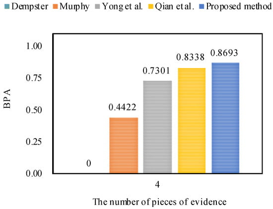
Figure 4.
The comparisons of target ’s BPA in terms of different methods.
6.2. Motor Rotor Fault Diagnosis
Supposing there are three types of faults for a motor rotor given by = , , in the frame of discernment U. We place a set of vibration acceleration sensors at different places for gathering the vibration signals given by S = . The acceleration vibration frequency amplitudes at , , and frequencies are considered as the fault feature variables. The collected sensor reports at , , and frequencies modeled as BPAs are shown in Table 7, Table 8 and Table 9, respectively, in which , , and represent the BPAs modeled from the three vibration acceleration sensors , , and .
Table 7.
The collected sensor reports at the frequency of modeled as BPAs.
Table 8.
The collected sensor reports at the frequency of modeled as BPAs.
Table 9.
The collected sensor reports at the frequency of modeled as BPAs.
6.2.1. Motor Rotor Fault Diagnosis at Frequency
By conducting the steps in Section 3, the weighted average evidence with regard to motor rotor fault diagnosis at frequency is obtained as below:
Then, the final fusion results for motor rotor fault diagnosis at frequency are computed as follows:
6.2.2. Motor Rotor Fault Diagnosis at Frequency
By carrying out the steps in Section 3, the weighted average evidence with respect to motor rotor fault diagnosis at frequency is obtained as follows:
Afterwards, the final fusion results in terms of motor rotor fault diagnosis at frequency are generated as below:
6.2.3. Motor Rotor Fault Diagnosis at Frequency
By applying the steps in Section 3, the weighted average evidence with respect to motor rotor fault diagnosis at frequency is obtained as follows:
Then, the final combination results for motor rotor fault diagnosis at frequency are shown below:
From the experimental results as shown in Table 10, Table 11 and Table 12, it can be seen that the proposed method diagnoses the fault type as , in accordance with Jiang et al.’s method [48].
Table 10.
Fusion results by using different combination methods at frequency.
Table 11.
Fusion results by using different combination methods at frequency.
Table 12.
Fusion results by using different combination methods at frequency.
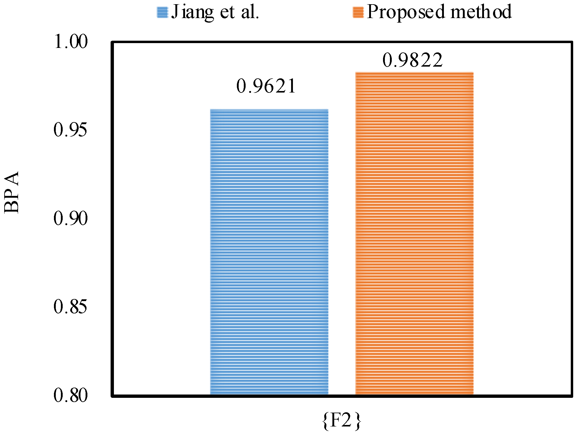
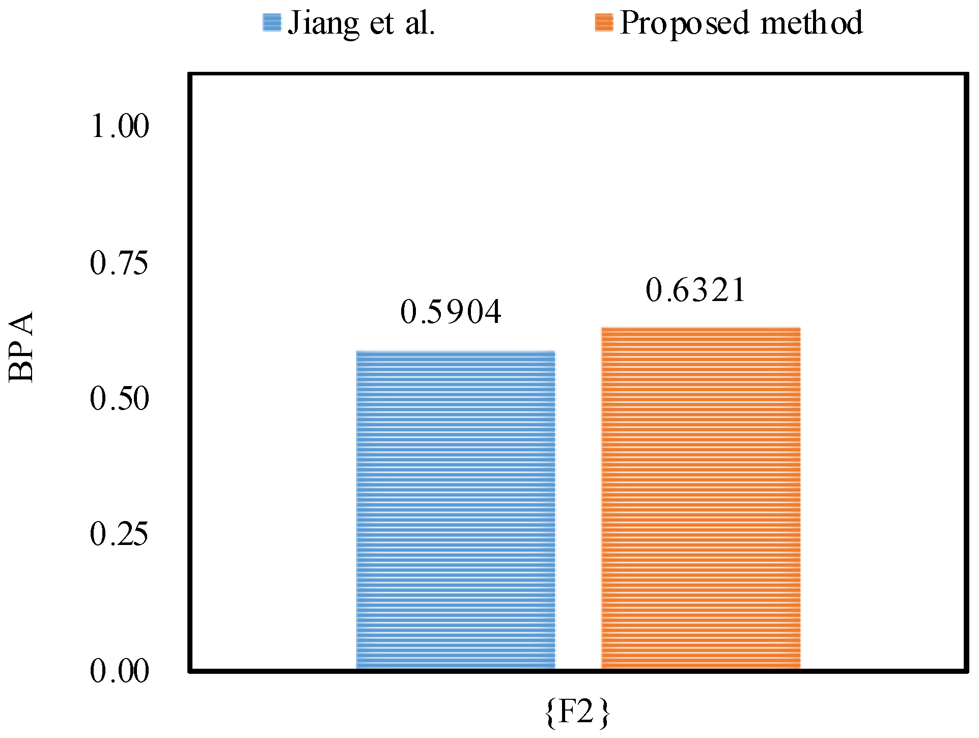
Furthermore, the proposed method outperforms Jiang et al.’s method [48] in dealing with the uncertainty as shown in Figure 5, Figure 6 and Figure 7, because by utilizing the proposed method, the belief degrees allocated to the target fault type at frequency, frequency and frequency increase up to 90.55%, 98.22%, and 63.21%, respectively; however, by using Jiang et al.’s method [48], the belief degrees allocated to the target at frequency, frequency and frequency are 88.61%, 96.21%, and 59.04%, respectively.
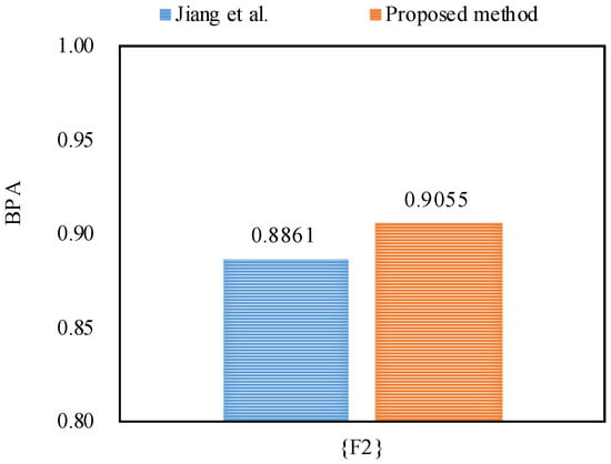
Figure 5.
The comparison of the BPA of the target at frequency.

Figure 6.
The comparison of the BPA of the target at frequency.

Figure 7.
The comparison of the BPA of the target at frequency.
Additionally, by utilizing the proposed method, the uncertainty falls from 0.0582 to 0.0541, and the uncertainty falls from 0.0555 to 0.0404 at frequency; the uncertainty decreased from 0.0371 to 0.0178 at frequency; the uncertainty falls from 0.0651 to 0.0333, and the uncertainty drops from 0.0061 to 0.0001 at frequency. As a result, the proposed method can diagnose motor rotor faults more accurately than the related work.
7. Conclusions
In this paper, a weighted combination method for conflicting evidence in multi-sensor data fusion was proposed by combining the modified cosine similarity measure of the pieces of evidence with the belief entropy function. The proposed method was a kind of pretreatment of the bodies of evidence, which was effective to handle the conflicting pieces of evidence in a multi-sensor environment. A numerical example was illustrated to show the feasibility and effectiveness of the proposal. In addition, applications in data classification and motor rotor fault diagnosis were presented to validate the practicability of the proposed method, where it outperformed the related methods with better accuracy.
Author Contributions
F.X. contributed most of the work in this paper. B.Q contributed the experiments in this paper.
Funding
“This research was funded by the National Natural Science Foundation of China grant numbers 61672435, 61702427, 61702426, and the 1000-Plan of Chongqing by Southwest University grant number SWU116007.”
Acknowledgments
The authors greatly appreciate the reviews’ suggestions and the editor’s encouragement.
Conflicts of Interest
The authors declare no conflict of interest.
References
- Jin, X.B.; Sun, Y.X. Pei-Radman fusion estimation algorithm for multisensor system applied in state monitoring. Lect. Notes Control Inf. Sci. 2006, 344, 963–968. [Google Scholar]
- Zadeh, L.A. Fuzzy sets. Inf. Control 1965, 8, 338–353. [Google Scholar] [CrossRef]
- Mardani, A.; Jusoh, A.; Zavadskas, E.K. Fuzzy multiple criteria decision-making techniques and applications–Two decades review from 1994 to 2014. Expert Syst. Appl. 2015, 42, 4126–4148. [Google Scholar] [CrossRef]
- Jiang, W.; Wei, B.; Liu, X.; Li, X.; Zheng, H. Intuitionistic fuzzy evidential power aggregation operator and its application in multiple criteria decision-making. Int. J. Syst. Sci. 2018, 49, 582–594. [Google Scholar] [CrossRef]
- Dempster, A.P. Upper and lower probabilities induced by a multivalued mapping. Ann. Math. Stat. 1967, 38, 325–339. [Google Scholar] [CrossRef]
- Shafer, G. A mathematical theory of evidence. Technometrics 1978, 20, 242. [Google Scholar] [CrossRef]
- Jiang, W.; Chang, Y.; Wang, S. A method to identify the incomplete framework of discernment in evidence theory. Math. Prob. Eng. 2017, 2017. [Google Scholar] [CrossRef]
- Walczak, B.; Massart, D. Rough sets theory. Chem. Intell. Lab. Syst. 1999, 47, 1–16. [Google Scholar] [CrossRef]
- Greco, S.; Matarazzo, B.; Slowinski, R. Rough sets theory for multicriteria decision analysis. Eur. J. Oper. Res. 2001, 129, 1–47. [Google Scholar] [CrossRef]
- Yang, J.B.; Xu, D.L. Evidential reasoning rule for evidence combination. Artif. Intell. 2013, 205, 1–29. [Google Scholar] [CrossRef]
- Fu, C.; Xu, D.L. Determining attribute weights to improve solution reliability and its application to selecting leading industries. Ann. Oper. Res. 2014, 245, 401–426. [Google Scholar] [CrossRef]
- Zadeh, L.A. A note on Z-numbers. Inf. Sci. 2011, 181, 2923–2932. [Google Scholar] [CrossRef]
- Kang, B.; Chhipi-Shrestha, G.; Deng, Y.; Hewage, K.; Sadiq, R. Stable Strategies Analysis Based on the Utility of Z-number in the Evolutionary Games. Appl. Math. Comput. 2018, 324, 202–217. [Google Scholar] [CrossRef]
- Bian, T.; Zheng, H.; Yin, L.; Deng, Y. Failure mode and effects analysis based on D numbers and TOPSIS. Qual. Reliab. Eng. Int. 2018. [Google Scholar] [CrossRef]
- Xiao, F. A novel multi-criteria decision making method for assessing health-care waste treatment technologies based on D numbers. Eng. Appl. Artif. Intell. 2018, 71, 216–225. [Google Scholar] [CrossRef]
- Xiao, F. An intelligent complex event processing with D numbers under fuzzy environment. Math. Prob. Eng. 2016, 2016. [Google Scholar] [CrossRef]
- Deng, X.; Deng, Y. D-AHP method with different credibility of information. Soft Comput. 2018. [Google Scholar] [CrossRef]
- Gao, Y.; Ran, C.J.; Sun, X.J.; Deng, Z.L. Optimal and self-tuning weighted measurement fusion Kalman filters and their asymptotic global optimality. Int. J. Adapt. Control Signal Process. 2010, 24, 982–1004. [Google Scholar] [CrossRef]
- Gao, Y.; Jia, W.J.; Sun, X.J.; Deng, Z.L. Self-tuning multisensor weighted measurement fusion Kalman filter. IEEE Trans. Aerosp. Electron. Syst. 2009, 45, 179–191. [Google Scholar]
- Jin, X.B.; Dou, C.; Su, T.L.; Lian, X.F.; Shi, Y. Parallel irregular fusion estimation based on nonlinear filter for indoor RFID tracking system. Int. J. Distrib. Sens. Netw. 2016, 2016, 1–11. [Google Scholar] [CrossRef]
- Zhou, X.; Hu, Y.; Deng, Y.; Chan, F.T.S.; Ishizaka, A. A DEMATEL-based completion method for incomplete pairwise comparison matrix in AHP. Ann. Oper. Res. 2018. [Google Scholar] [CrossRef]
- Xu, H.; Deng, Y. Dependent evidence combination based on Shearman coefficient and Pearson coefficient. IEEE Access 2018, 6, 11634–11640. [Google Scholar] [CrossRef]
- Dutta, P. Uncertainty modeling in risk assessment based on Dempster–Shafer theory of evidence with generalized fuzzy focal elements. Fuzzy Inf. Eng. 2015, 7, 15–30. [Google Scholar] [CrossRef]
- Liu, T.; Deng, Y.; Chan, F. Evidential supplier selection based on DEMATEL and game theory. Int. J. Fuzzy Syst. 2018, 20, 1321–1333. [Google Scholar] [CrossRef]
- Denoeux, T. A k-nearest neighbor classification rule based on Dempster–Shafer theory. IEEE Trans. Syst. Man Cybern. 1995, 25, 804–813. [Google Scholar] [CrossRef]
- Liu, Z.; Quan, P.; Dezert, J.; Han, J.W.; You, H. Classifier fusion with contextual reliability evaluation. IEEE Trans. Cybern. 2017, PP, 1–14. [Google Scholar] [CrossRef] [PubMed]
- Zheng, X.; Deng, Y. Dependence assessment in human reliability analysis based on evidence credibility decay model and IOWA operator. Ann. Nuclear Energy 2018, 112, 673–684. [Google Scholar] [CrossRef]
- Xiao, F. A novel evidence theory and fuzzy preference approach-based multi-sensor data fusion technique for fault diagnosis. Sensors 2017, 17, 2504. [Google Scholar] [CrossRef] [PubMed]
- Jiang, W.; Wang, S. An uncertainty measure for interval-valued evidences. Int. J. Comput. Commun. Control 2017, 12, 631–644. [Google Scholar] [CrossRef]
- Xiao, F. An improved method for combining conflicting evidences Based on the similarity measure and belief function entropy. Int. J. Fuzzy Syst. 2017, 1–11. [Google Scholar] [CrossRef]
- Zheng, H.; Deng, Y. Evaluation method based on fuzzy relations between Dempster-Shafer belief structure. Int. J. Intell. Syst. 2017. [Google Scholar] [CrossRef]
- Jiang, W.; Yang, T.; Shou, Y.; Tang, Y.; Hu, W. Improved evidential fuzzy c-means method. J. Syst. Eng. Electron. 2018, 29, 187–195. [Google Scholar]
- Zadeh, L.A. A simple view of the Dempster–Shafer theory of evidence and its implication for the rule of combination. AI Mag. 1986, 7, 85–90. [Google Scholar]
- Lefevre, E.; Colot, O.; Vannoorenberghe, P. Belief function combination and conflict management. Inf. Fusion 2002, 3, 149–162. [Google Scholar] [CrossRef]
- Deng, X.; Jiang, W. An evidential axiomatic design approach for decision making using the evaluation of belief structure satisfaction to uncertain target values. Int. J. Intell. Syst. 2018, 33, 15–32. [Google Scholar] [CrossRef]
- Jiang, W.; Hu, W. An improved soft likelihood function for Dempster-Shafer belief structures. Int. J. Intell. Syst. 2018. [Google Scholar] [CrossRef]
- Smets, P. The combination of evidence in the transferable belief model. IEEE Trans. Pattern Anal. Mach. Intell. 1990, 12, 447–458. [Google Scholar] [CrossRef]
- Dubois, D.; Prade, H. Representation and combination of uncertainty with belief functions and possibility measures. Comput. Intell. 1988, 4, 244–264. [Google Scholar] [CrossRef]
- Yager, R.R. On the Dempster–Shafer framework and new combination rules. Inf. Sci. 1987, 41, 93–137. [Google Scholar] [CrossRef]
- Murphy, C.K. Combining belief functions when evidence conflicts. Decis. Support Syst. 2000, 29, 1–9. [Google Scholar] [CrossRef]
- Deng, Y.; Shi, W.; Zhu, Z.; Liu, Q. Combining belief functions based on distance of evidence. Decis. Support Syst. 2004, 38, 489–493. [Google Scholar]
- Jiang, W.; Wei, B.; Qin, X.; Zhan, J.; Tang, Y. Sensor data fusion based on a new conflict measure. Math. Prob. Eng. 2016, 2016. [Google Scholar] [CrossRef]
- Deng, Y. Deng entropy. Chaos Solitons Fractals 2016, 91, 549–553. [Google Scholar] [CrossRef]
- Khaleghi, B.; Khamis, A.; Karray, F.O.; Razavi, S.N. Multisensor data fusion: A review of the state-of-the-art. Inf. Fusion 2013, 14, 28–44. [Google Scholar] [CrossRef]
- Niu, G.; Yang, B.S.; Pecht, M. Development of an optimized condition-based maintenance system by data fusion and reliability-centered maintenance. Reliab. Eng. Syst. Saf. 2010, 95, 786–796. [Google Scholar] [CrossRef]
- Yunusa-Kaltungo, A.; Sinha, J.K. Sensitivity analysis of higher order coherent spectra in machine faults diagnosis. Struct. Health Monit. 2016, 15, 555–567. [Google Scholar] [CrossRef]
- Yunusa-Kaltungo, A.; Sinha, J.K.; Nembhard, A.D. A novel fault diagnosis technique for enhancing maintenance and reliability of rotating machines. Struct. Health Monit. 2015, 14, 231–262. [Google Scholar] [CrossRef]
- Jiang, W.; Xie, C.; Zhuang, M.; Shou, Y.; Tang, Y. Sensor data fusion with Z-numbers and its application in fault diagnosis. Sensors 2016, 16, 1509. [Google Scholar] [CrossRef] [PubMed]
- Akselrod, D.; Sinha, A.; Kirubarajan, T. Information flow control for collaborative distributed data fusion and multisensor multitarget tracking. IEEE Trans. Syst. Man Cybern. Part C 2012, 42, 501–517. [Google Scholar] [CrossRef]
- Dallil, A.; Oussalah, M.; Ouldali, A. Sensor fusion and target tracking using evidential data association. IEEE Sens. J. 2013, 13, 285–293. [Google Scholar] [CrossRef]
- Kashanian, H.; Dabaghi, E. Feature dimension reduction of multisensor data fusion using principal component fuzzy analysis. Int. J. Eng. 2017, 30, 493–499. [Google Scholar]
- Hernandez-Penaloza, G.; Belmonte-Hernandez, A.; Quintana, M.; Alvarez, F. A Multi-sensor Fusion Scheme to Increase Life Autonomy of Elderly People with Cognitive Problems. IEEE Access 2018, 6, 12775–12789. [Google Scholar] [CrossRef]
- Santos, E.N.D.; Silva, M.J.D. Advanced image processing of wire-mesh sensor data for two-phase flow investigation. IEEE Latin Am. Trans. 2015, 13, 2269–2277. [Google Scholar] [CrossRef]
- Mohammadi, A.; Yang, C.; Chen, Q.W. Attack detection/isolation via a secure multisensor fusion framework for cyberphysical systems. Complexity 2018, 2018, 1–8. [Google Scholar] [CrossRef]
- Santi, F.; Pastina, D.; Bucciarelli, M. Estimation of ship dynamics with a multi-platform Radar imaging system. IEEE Trans. Aerosp. Electron. Syst. 2017, 53, 2769–2788. [Google Scholar] [CrossRef]
- Geiß, C.; Thoma, M.; Pittore, M.; Wieland, M.; Dech, S.W.; Taubenbock, H. Multitask active learning for characterization of built environments with multisensor earth observation data. IEEE J. Sel. Top. Appl. Earth Obs. Remote Sens. 2017, PP, 1–15. [Google Scholar]
- Zhang, Q.; Li, M.; Deng, Y. Measure the structure similarity of nodes in complex networks based on relative entropy. Phys. A Stat. Mech. Appl. 2018, 491, 749–763. [Google Scholar] [CrossRef]
- Jiang, W.; Wei, B.; Liu, X.; Li, X.; Zheng, H. Intuitionistic fuzzy power aggregation operator based on entropy and its application in decision making. Int. J. Intell. Syst. 2018, 33, 49–67. [Google Scholar] [CrossRef]
- Qian, J.; Guo, X.; Deng, Y. A novel method for combining conflicting evidences based on information entropy. Appl. Intell. 2017, 46, 876–888. [Google Scholar] [CrossRef]


© 2018 by the authors. Licensee MDPI, Basel, Switzerland. This article is an open access article distributed under the terms and conditions of the Creative Commons Attribution (CC BY) license (http://creativecommons.org/licenses/by/4.0/).