Ultrasonic Phased Array Compressive Imaging in Time and Frequency Domain: Simulation, Experimental Verification and Real Application

Abstract
:
1. Introduction
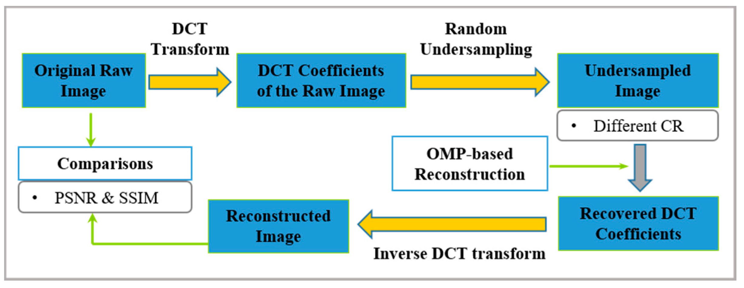
2. Overview of CS
2.1. Sparsity of Transform Coding
2.2. Measurement with Incoherence
2.3. Reconstruction via Optimization
| Algorithm 1 Orthogonal Matching Pursuit (OMP) |
| Input: A signal , a matrix . Initialize: Set the support set , the residual error and put the counter . Identify: Find a column from A that most correlates with the residual error and record the correlation coefficient: Output: The vector with components and otherwise. |
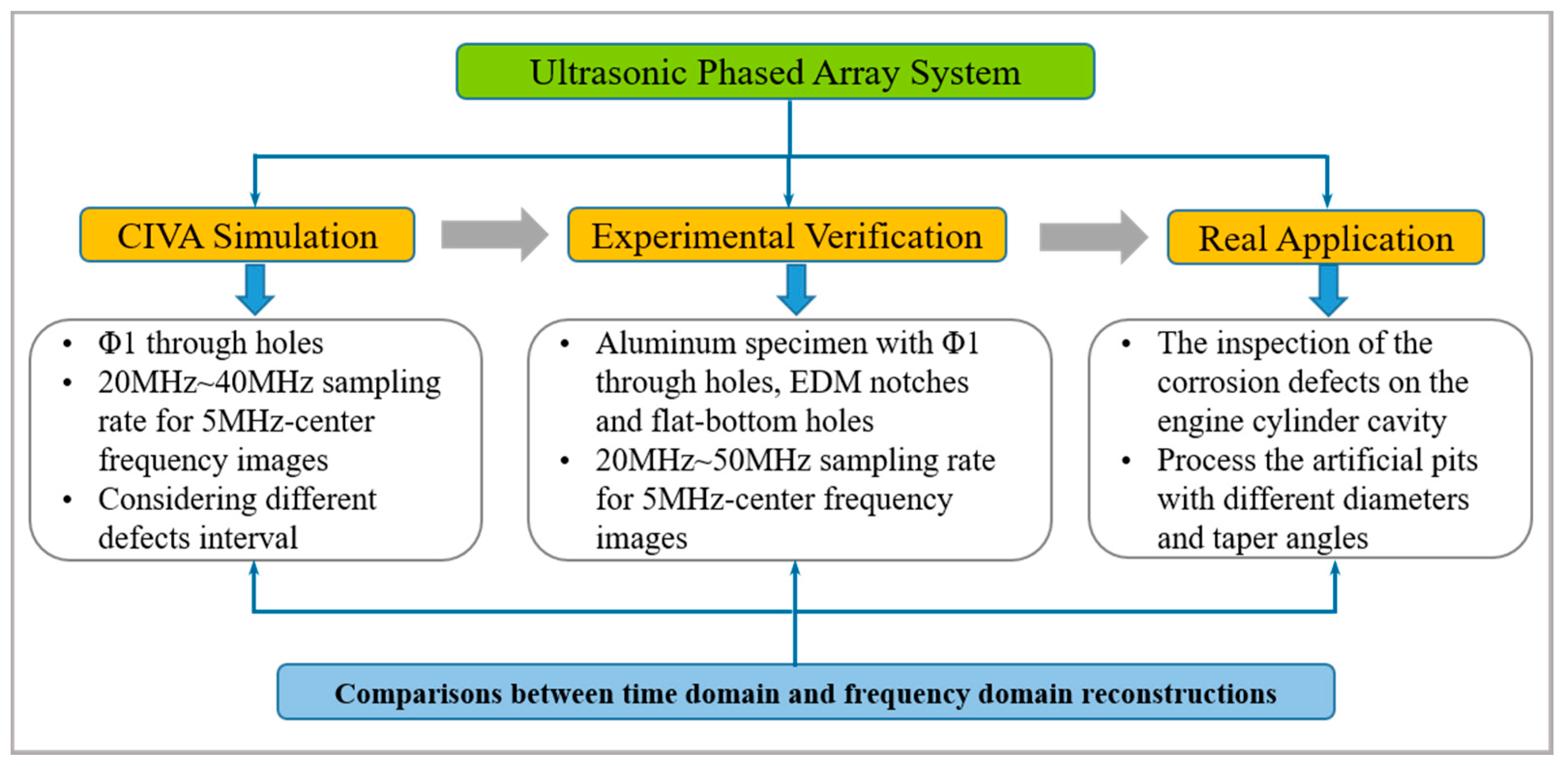
3. Simulation Results and Discussion
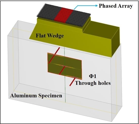
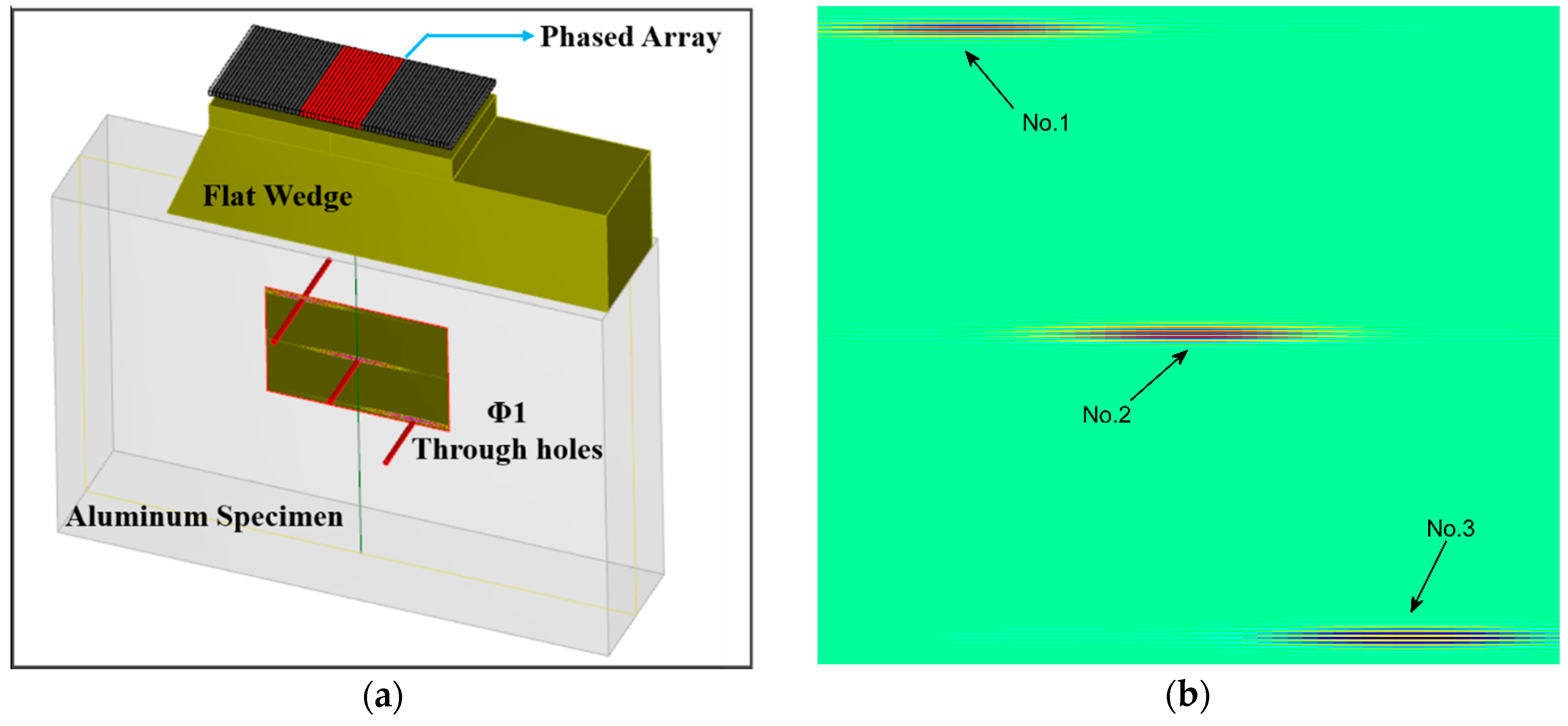
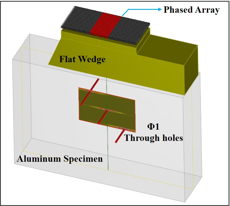
3.1. Simulation Settings
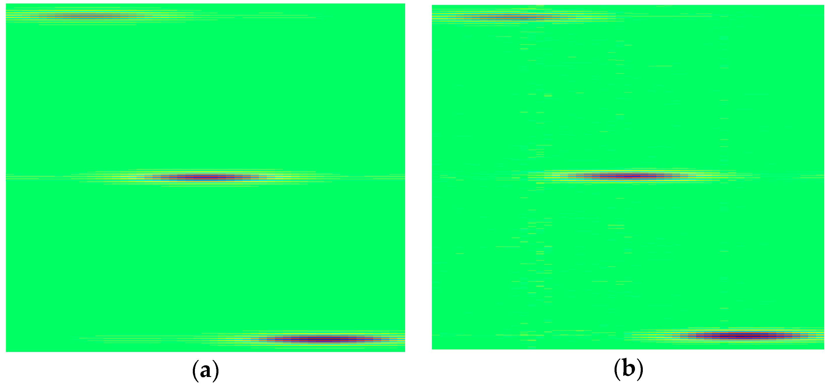
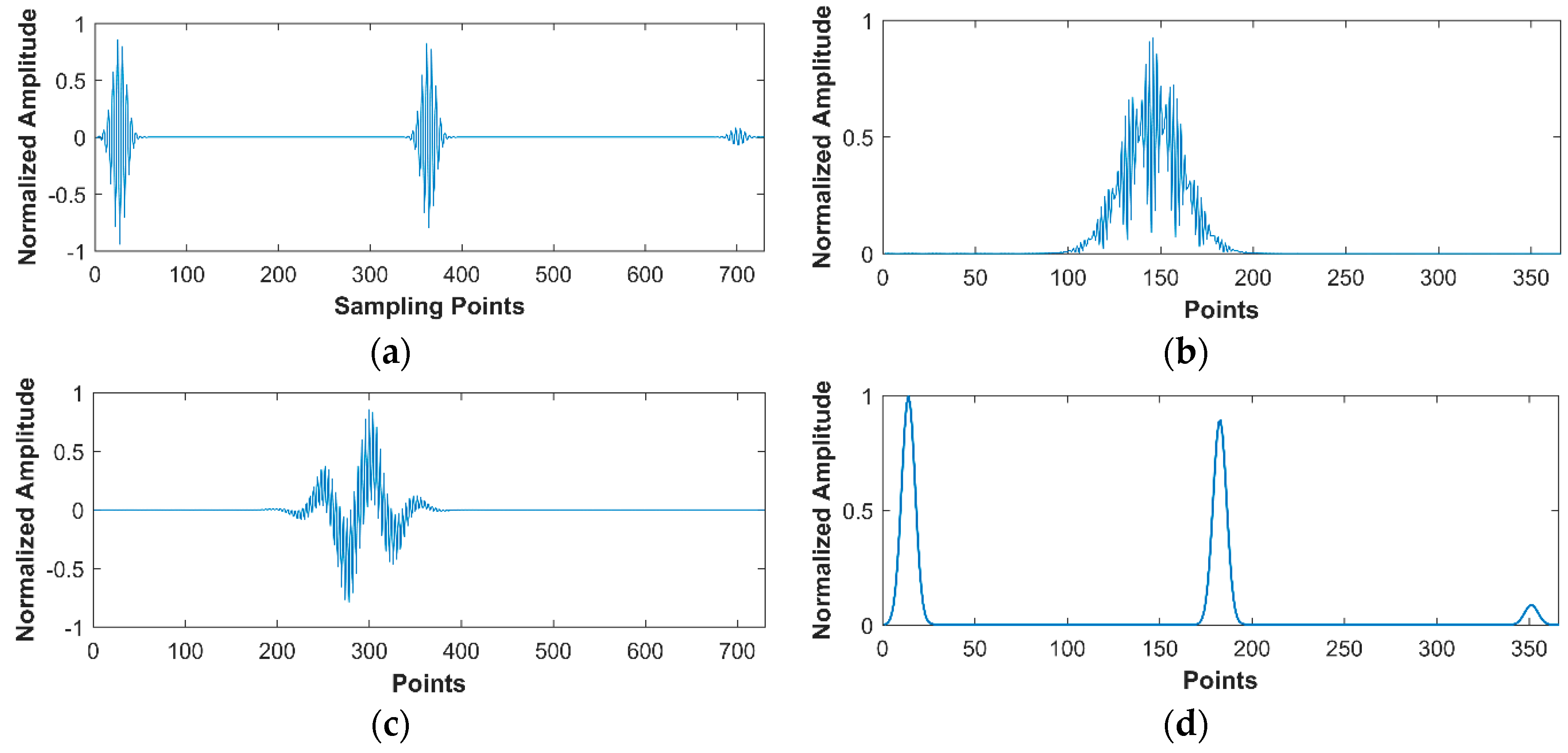
3.2. Time Domain Reconstructions
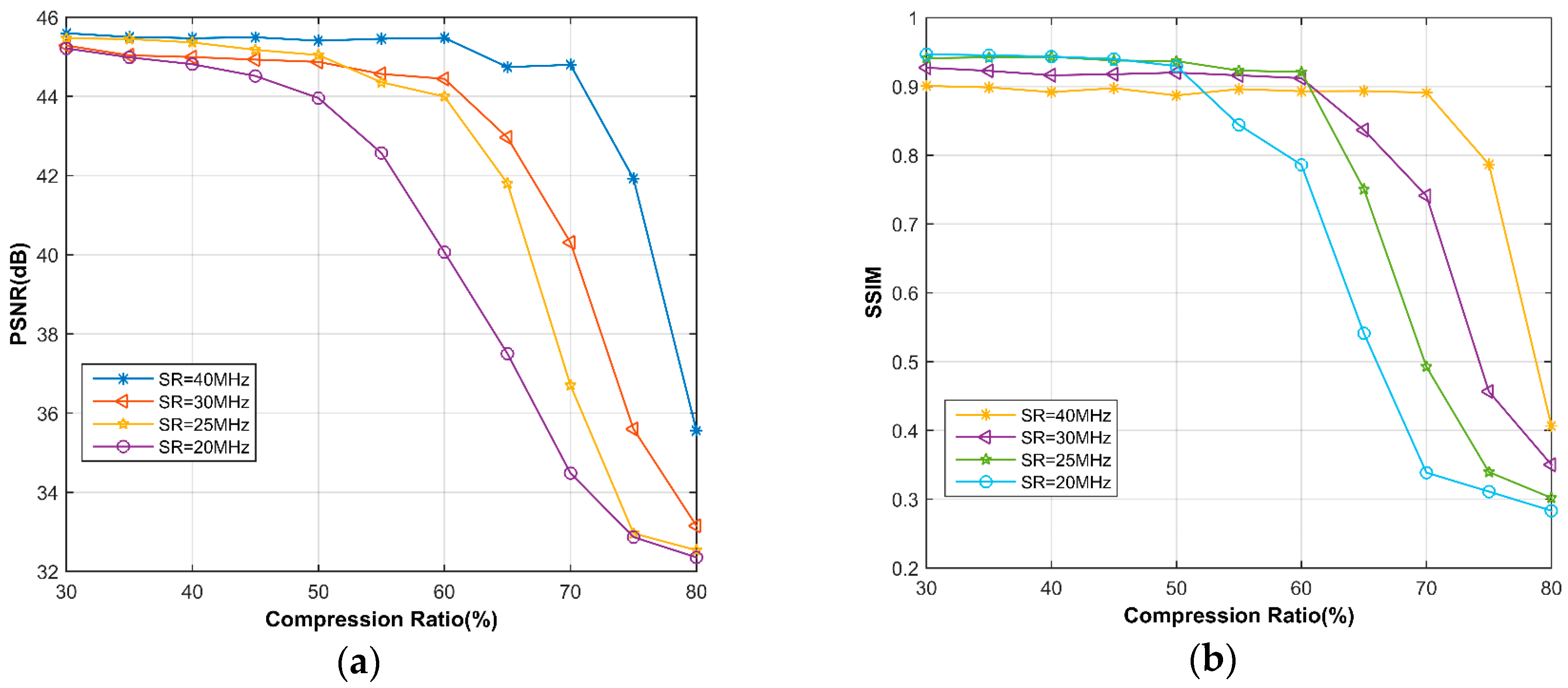
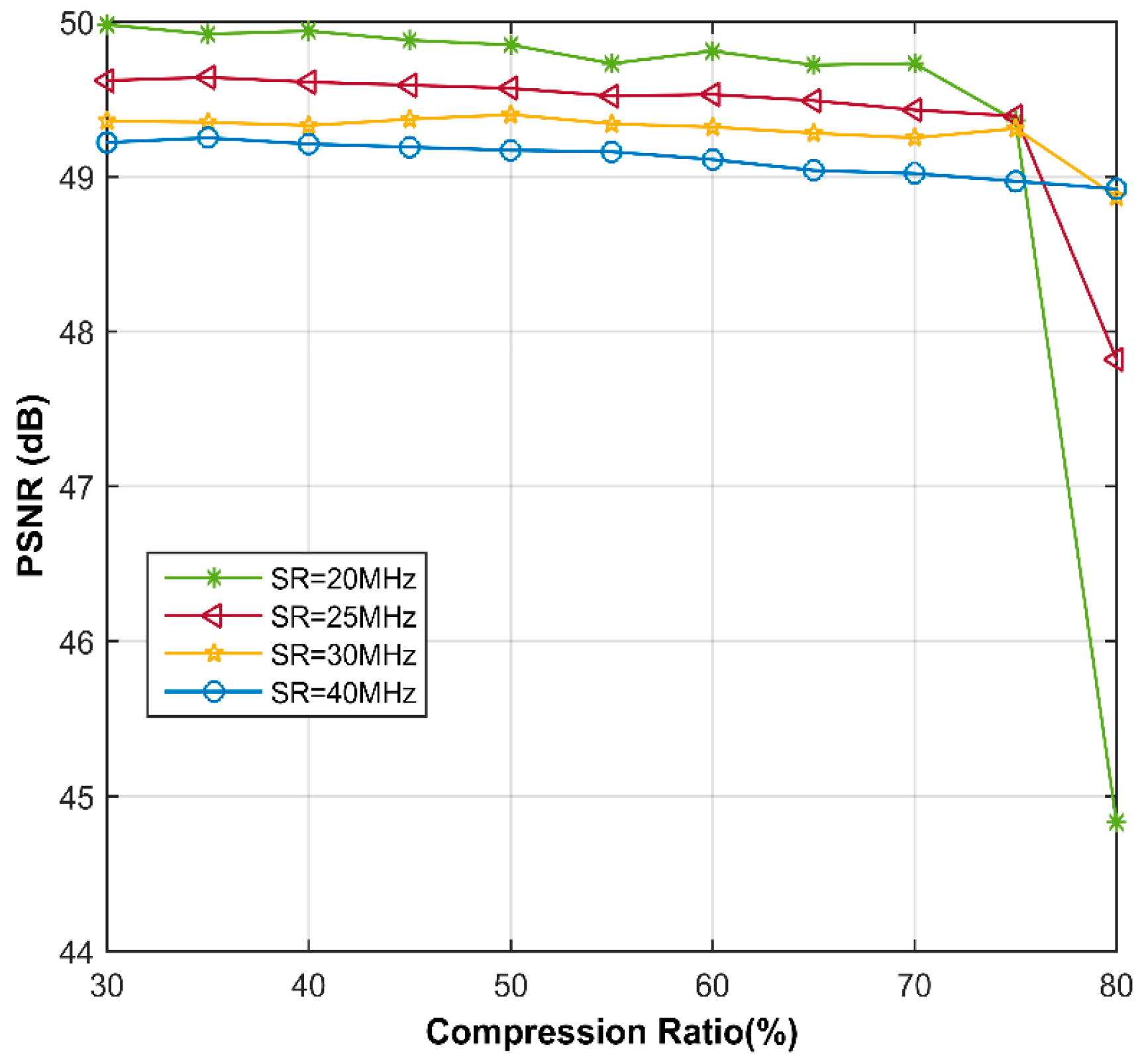
3.3. Frequency Domain Reconstructions
4. Experimental Results and Discussion
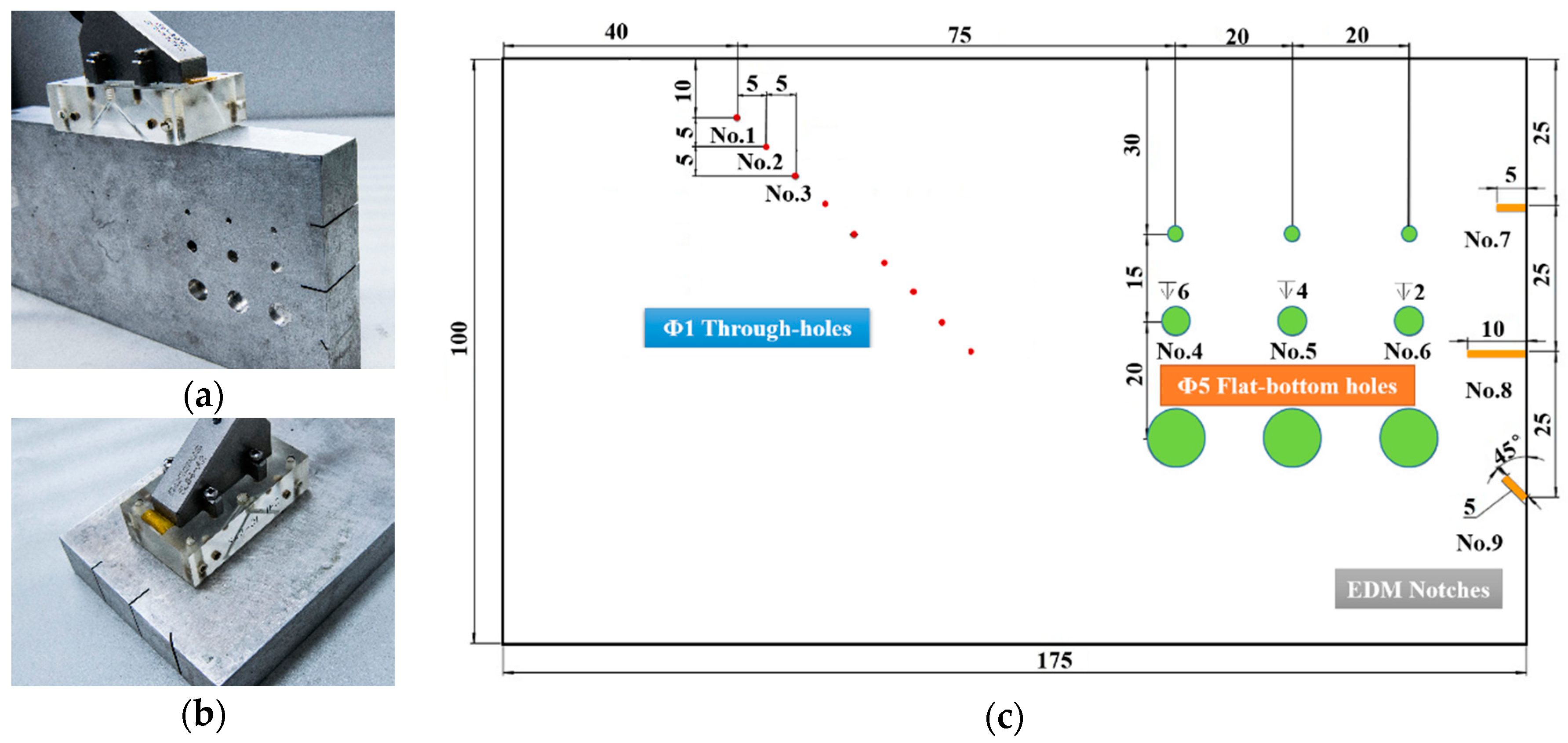
4.1. Apparatus, Real-Time Images and Algorithm Parameters
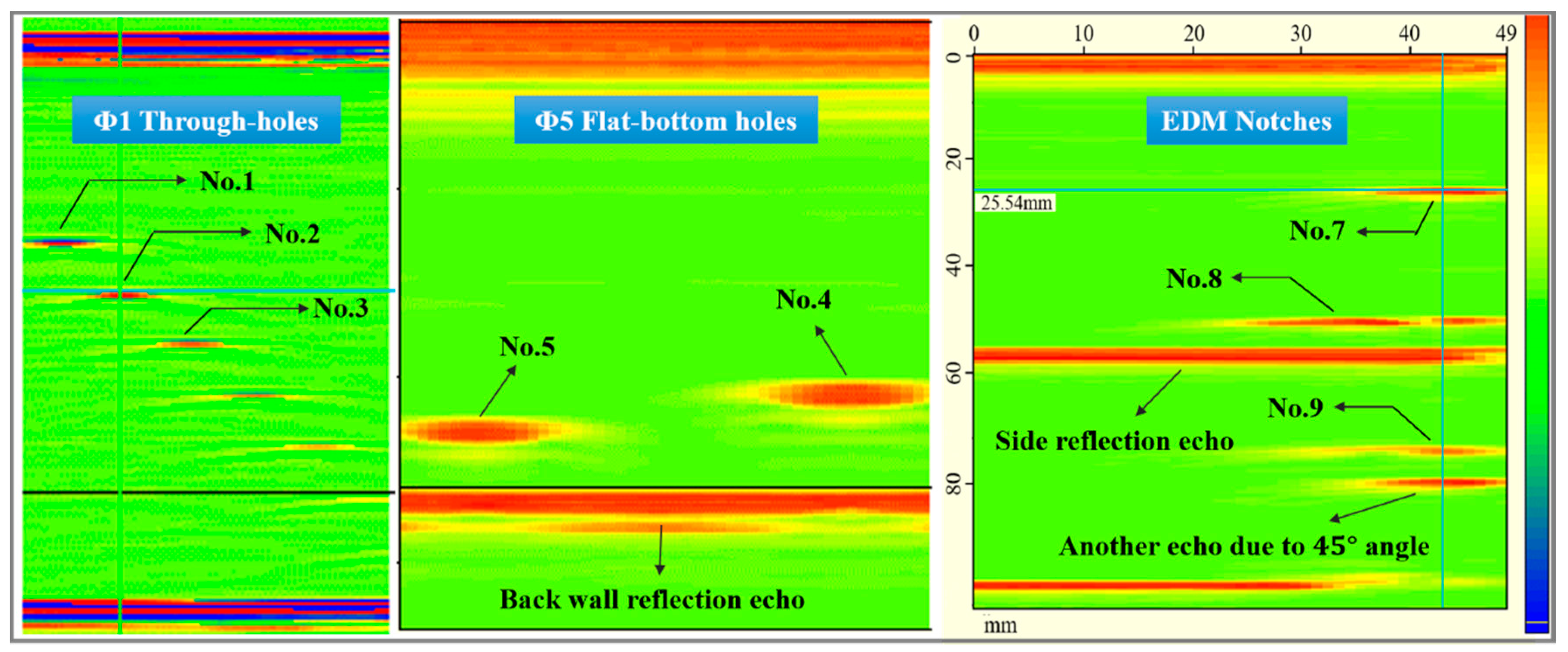
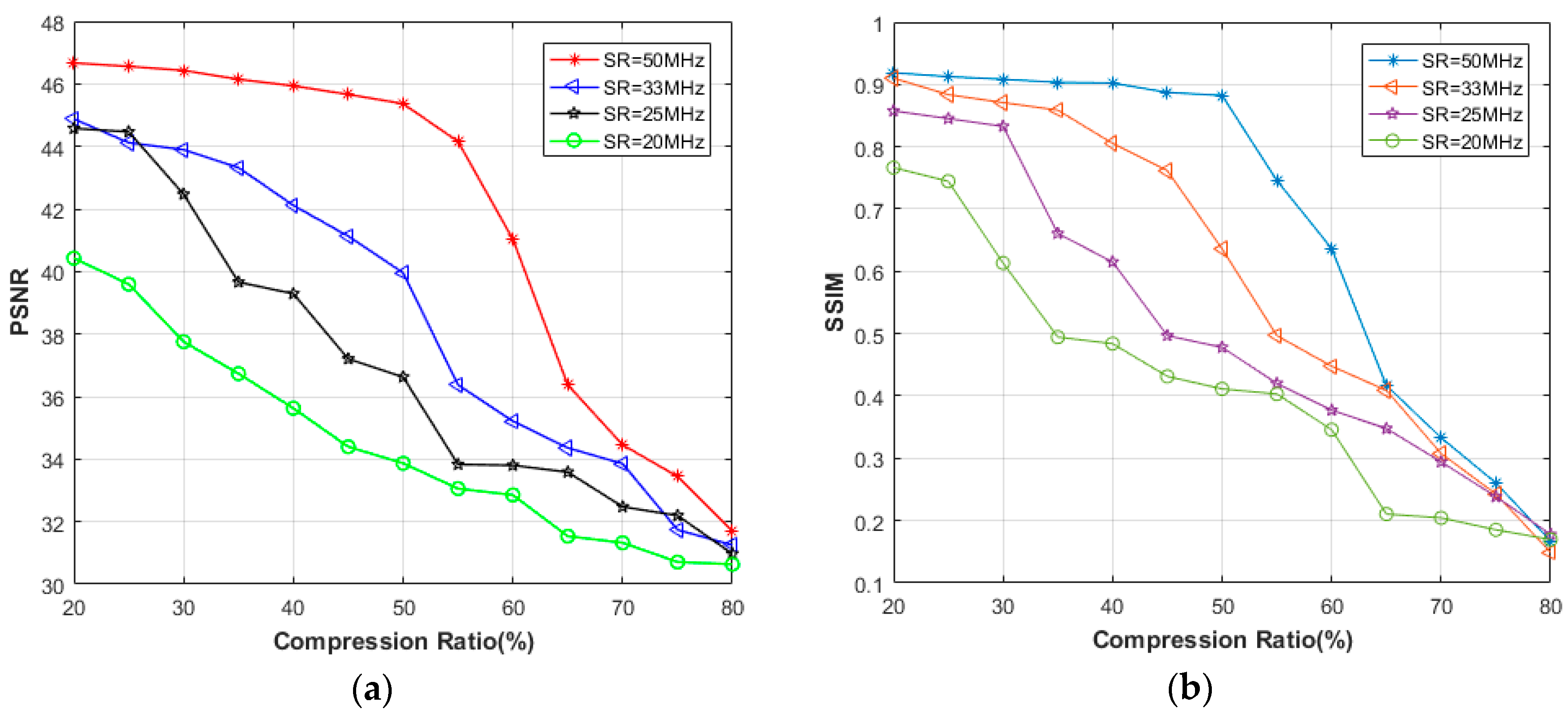
4.2. Time Domain Reconstructions
4.3. Frequency Domain Reconstructions
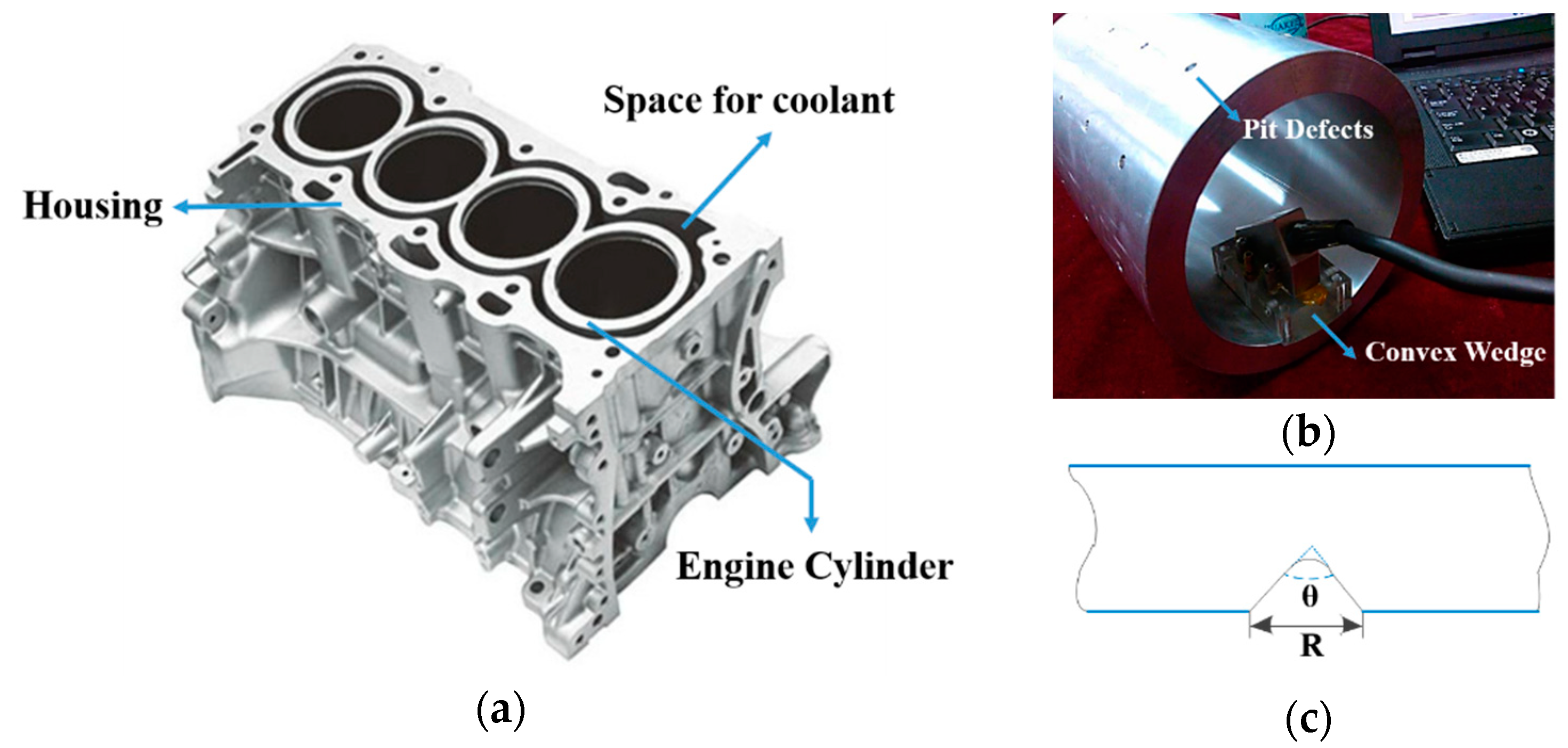
4.4. Real Application in Engine Cylinder Cavity Inspection
5. Conclusions
Author Contributions
Funding
Acknowledgments
Conflicts of Interest
References
- Drinkwater, B.W.; Wilcox, P.D. Ultrasonic arrays for non-destructive evaluation: A review. NDT E Int. 2006, 39, 525–541. [Google Scholar] [CrossRef]
- Yang, X.; Chen, S.; Jin, S.; Chang, W. Crack orientation and depth estimation in a low-pressure turbine disc using a phased array ultrasonic transducer and an artificial neural network. Sensors 2013, 13, 12375–12391. [Google Scholar] [CrossRef] [PubMed]
- Yang, S.; Yoon, B.; Kim, Y. Using phased array ultrasonic technique for the inspection of straddle mount-type low-pressure turbine disc. NDT E Int. 2009, 42, 128–132. [Google Scholar] [CrossRef]
- Brunelli, D.; Caione, C. Sparse recovery optimization in wireless sensor networks with a sub-nyquist sampling rate. Sensors 2015, 15, 16654–16673. [Google Scholar] [CrossRef] [PubMed]
- Gao, F.; Zeng, L.; Lin, J.; Luo, Z. Mode separation in frequency-wavenumber domain through compressed sensing of far-field Lamb waves. Meas. Sci. Technol. 2017, 28, 075004. [Google Scholar] [CrossRef]
- Wang, Y.; Duan, X.; Tian, D.; Zhou, J.; Lu, Y.; Lu, G. A Bayesian compressive sensing vehicular location method based on three-dimensional radio frequency. Int. J. Distrib. Sens. Netw. 2014, 10, 1–13. [Google Scholar] [CrossRef]
- Bao, Y.; Li, H.; Sun, X.; Yu, Y.; Qu, J. Compressive sampling–based data loss recovery for wireless sensor networks used in civil structural health monitoring. Struct. Health Monit. 2013, 12, 78–95. [Google Scholar] [CrossRef]
- Candès, E.J.; Wakin, M.B. An introduction to compressive sampling. IEEE Signal. Proc. Mag. 2008, 25, 21–30. [Google Scholar] [CrossRef]
- Pareschi, F.; Albertini, P.; Frattini, G.; Mangia, M.; Rovatti, R.; Setti, G. Hardware-algorithms co-design and implementation of an analog-to-information converter for biosignals based on compressed sensing. IEEE Trans. Biomed. Circuits Syst. 2016, 10, 149–162. [Google Scholar] [CrossRef] [PubMed]
- Wagner, N.; Eldar, Y.C.; Friedman, Z. Compressed beamforming in ultrasound imaging. IEEE Trans. Signal. Proc. 2012, 60, 4643–4657. [Google Scholar] [CrossRef]
- Lorintiu, O.; Liebgott, H.; Martino, A.; Bernard, O.; Friboulet, D. Compressed sensing reconstruction of 3D ultrasound data using dictionary learning and line-wise subsampling. In Proceedings of the IEEE International Conference on Image Processing (ICIP), Paris, France, 27–30 October 2014; pp. 2467–2477. [Google Scholar]
- Liebgott, H.; Prost, R.; Friboulet, D. Pre-beamformed RF signal reconstruction in medical ultrasound using compressive sensing. Ultrasonics 2013, 53, 525–533. [Google Scholar] [CrossRef] [PubMed]
- Foroozan, F.; Sadeghi, P. Wave atom based Compressive Sensing and adaptive beamforming in ultrasound imaging. In Proceedings of the IEEE International Conference on Acoustics, Speech and Signal Processing, Brisbane, Australia, 19–24 April 2015; pp. 2474–2478. [Google Scholar]
- Liebgott, H.; Adrian, B.; Denis, K.; Olivier, B.; Denis, F. Compressive sensing in medical ultrasound. In Proceedings of the IEEE International Ultrasonics Symposium, Dresden, Germany, 7–10 October 2012; pp. 1–6. [Google Scholar]
- López, Y.Á.; Lorenzo, J.Á. Compressed sensing techniques applied to ultrasonic imaging of cargo containers. Sensors 2017, 17, 162. [Google Scholar] [CrossRef] [PubMed]
- Di, I.T.; De, M.L.; Perelli, A.; Marzani, A. Compressive sensing of full wave field data for structural health monitoring applications. IEEE Trans. Ultrason. Ferroelectr. Freq. Control 2015, 62, 1373–1383. [Google Scholar]
- Mesnil, O.; Ruzzene, M. Sparse wavefield reconstruction and source detection using Compressed Sensing. Ultrasonics 2016, 67, 94–104. [Google Scholar] [CrossRef] [PubMed]
- Wang, W.; Bao, Y.; Zhou, W.; Li, H. Sparse representation for Lamb-wave-based damage detection using a dictionary algorithm. Ultrasonics 2018, 87, 48–58. [Google Scholar] [CrossRef] [PubMed]
- Sun, Y.; Gu, F. Compressive sensing of piezoelectric sensor response signal for phased array structural health monitoring. Int. J. Sens. Netw. 2017, 23, 258–264. [Google Scholar] [CrossRef]
- Wang, W.; Zhang, H.; Lynch, J.P.; Cesnik, C.E.; Li, H. Experimental and numerical validation of guided wave phased arrays integrated within standard data acquisition systems for structural health monitoring. Struct. Control Health 2018, e2171. [Google Scholar] [CrossRef]
- Chernyakova, T.; Eldar, Y.C. Fourier-domain beamforming: The path to compressed ultrasound imaging. IEEE Trans. Ultrason. Ferroelectr. Freq. Control 2014, 61, 1252–1267. [Google Scholar] [CrossRef] [PubMed]
- Burshtein, A.; Birk, M.; Chernyakova, T.; Eilam, A.; Kempinski, A.; Eldar, Y.C. Sub-Nyquist sampling and Fourier domain beamforming in volumetric ultrasound imaging. IEEE Trans. Ultrason. Ferroelectr. Freq. Control 2016, 63, 703–716. [Google Scholar] [CrossRef] [PubMed]
- Mishra, P.K.; Bharath, R.; Rajalakshmi, P.; Desai, U.B. Compressive sensing ultrasound beamformed imaging in time and frequency domain. In Proceedings of the International Conference on E-Health Networking, Application & Services, Boston, MA, USA, 14–17 October 2015; pp. 523–527. [Google Scholar]
- Rauhut, H.; Schnass, K.; Vandergheynst, P. Compressed sensing and redundant dictionaries. IEEE Trans. Inf. Theory 2008, 54, 2210–2219. [Google Scholar] [CrossRef]
- Baraniuk, R.G. Compressive sensing. IEEE Signal. Proc. Mag. 2007, 24, 118–121. [Google Scholar] [CrossRef]
- Candès, E.J.; Eldar, Y.C.; Needell, D.; Randall, P. Compressed sensing with coherent and redundant dictionaries. Appl. Comput. Harmonic Anal. 2011, 31, 59–73. [Google Scholar] [CrossRef]
- Tropp, J.A.; Wright, S.J. Computational methods for sparse solution of linear inverse problems. Proc. IEEE 2010, 98, 948–958. [Google Scholar] [CrossRef]
- Calmon, P. Trends and stakes of NDT simulation. J. Nondestruct. Eval. 2012, 31, 339–341. [Google Scholar] [CrossRef]
- Calmon, P.; Mahaut, S.; Chatillon, S.; Raillon, R. CIVA: An expertise platform for simulation and processing NDT data. Ultrasonics 2006, 44, e975–e979. [Google Scholar] [CrossRef] [PubMed]
- Achim, A.; Buxton, B.; Tzagkarakis, G.; Tsakalides, P. Compressive sensing for ultrasound RF echoes using a-stable distributions. In Proceedings of the International Conference of the IEEE Engineering in Medicine and Biology Society, Buenos Aires, Argentina, 31 August–4 September 2010; pp. 4304–4307. [Google Scholar]
- Wang, Z.; Bovik, A.C.; Sheikh, H.R.; Simoncelli, E.P. Image quality assessment: From error visibility to structural similarity. IEEE Trans. Image Process. 2004, 13, 600–612. [Google Scholar] [CrossRef] [PubMed]
- Yang, X.; Xue, B.; Jia, L.; Zhang, H. Quantitative analysis of pit defects in an automobile engine cylinder cavity using the radial basis function neural network-genetic algorithm model. Struct. Health Monit. 2017, 16, 696–710. [Google Scholar] [CrossRef]
- Yang, X.; Chen, S.; Sun, F.; Jin, S.; Chang, W. Simulation study on the acoustic field from linear phased array ultrasonic transducer for engine cylinder testing. CMES Comput. Model. Eng. Sci. 2013, 90, 487–500. [Google Scholar]


| Array Parameter | Value |
|---|---|
| Center Frequency | 5 MHz |
| Element Count | 64 |
| Element Pitch | 0.60 mm |
| Element Width | 0.50 mm |
| Element Elevation | 10.0 mm |
| Pulse Type | Gaussian weighted |
| −6 dB Bandwidth | 50% |
| Measurement Points | 200 | 220 | 240 | 260 | 280 | 300 | 320 | 340 |
|---|---|---|---|---|---|---|---|---|
| 20 MHz SR (584 points) | 37.50 | 38.45 | 40.59 | 42.57 | 43.92 | 43.98 | 44.37 | 44.57 |
| 25 MHz SR (730 points) | 34.99 | 37.56 | 37.65 | 41.06 | 43.83 | 44.19 | 44.23 | 44.44 |
| 30 MHz SR (876 points) | 34.31 | 35.60 | 37.14 | 39.81 | 42.22 | 44.19 | 44.23 | 44.39 |
| 40 MHz SR (1168 points) | 32.35 | 33.99 | 35.70 | 39.38 | 43.81 | 44.13 | 44.28 | 44.53 |
| CR (%) | 20 | 30 | 40 | 50 | 60 | 70 | 80 | |
|---|---|---|---|---|---|---|---|---|
| 20 MHz SR | σ | 0.4322 | 0.3878 | 0.4217 | 0.3930 | 0.4593 | 6.4072 | 9.3127 |
| Fit 3σ criterion | √ | √ | √ | √ | √ | X | X | |
| 25 MHz SR | σ | 0.3677 | 0.4539 | 0.3876 | 0.4211 | 0.4125 | 4.5018 | 5.3882 |
| Fit 3σ criterion | √ | √ | √ | √ | √ | X | X | |
| 33 MHz SR | σ | 0.4482 | 0.3975 | 0.4421 | 0.3903 | 0.3759 | 0.5225 | 3.5697 |
| Fit 3σ criterion | √ | √ | √ | √ | √ | √ | X | |
| 50 MHz SR | σ | 0.3855 | 0.4203 | 0.3547 | 0.3971 | 0.3632 | 0.4125 | 3.4338 |
| Fit 3σ criterion | √ | √ | √ | √ | √ | √ | X |
| Measurement Points | 160 | 180 | 200 | 220 | 240 | 260 | 280 | 300 |
|---|---|---|---|---|---|---|---|---|
| 25 MHz SR (256 points) | 39.44 | 42.47 | 44.47 | 44.52 | 44.63 | N/A | N/A | N/A |
| 33 MHz SR (341 points) | 36.61 | 41.04 | 42.10 | 43.32 | 43.89 | 44.68 | 45.19 | 45.31 |
| 50 MHz SR (512 points) | 34.82 | 36.37 | 41.01 | 42.51 | 43.56 | 45.36 | 45.66 | 45.87 |
| No. | 1 | 2 | 3 | 4 | 5 | 6 | 7 | 8 | 9 | 10 | 11 | 12 |
|---|---|---|---|---|---|---|---|---|---|---|---|---|
| R (mm) | 2 | 3 | 4 | 5 | 2 | 3 | 4 | 5 | 2 | 3 | 4 | 5 |
| θ (°) | 120 | 120 | 120 | 120 | 90 | 90 | 90 | 90 | 60 | 60 | 60 | 60 |
© 2018 by the authors. Licensee MDPI, Basel, Switzerland. This article is an open access article distributed under the terms and conditions of the Creative Commons Attribution (CC BY) license (http://creativecommons.org/licenses/by/4.0/).
Share and Cite
Bai, Z.; Chen, S.; Jia, L.; Zeng, Z. Ultrasonic Phased Array Compressive Imaging in Time and Frequency Domain: Simulation, Experimental Verification and Real Application. Sensors 2018, 18, 1460. https://doi.org/10.3390/s18051460
Bai Z, Chen S, Jia L, Zeng Z. Ultrasonic Phased Array Compressive Imaging in Time and Frequency Domain: Simulation, Experimental Verification and Real Application. Sensors. 2018; 18(5):1460. https://doi.org/10.3390/s18051460
Chicago/Turabian StyleBai, Zhiliang, Shili Chen, Lecheng Jia, and Zhoumo Zeng. 2018. "Ultrasonic Phased Array Compressive Imaging in Time and Frequency Domain: Simulation, Experimental Verification and Real Application" Sensors 18, no. 5: 1460. https://doi.org/10.3390/s18051460
APA StyleBai, Z., Chen, S., Jia, L., & Zeng, Z. (2018). Ultrasonic Phased Array Compressive Imaging in Time and Frequency Domain: Simulation, Experimental Verification and Real Application. Sensors, 18(5), 1460. https://doi.org/10.3390/s18051460