Quantitative Study on Corrosion of Steel Strands Based on Self-Magnetic Flux Leakage


Abstract
:1. Introduction
2. Theoretical Background
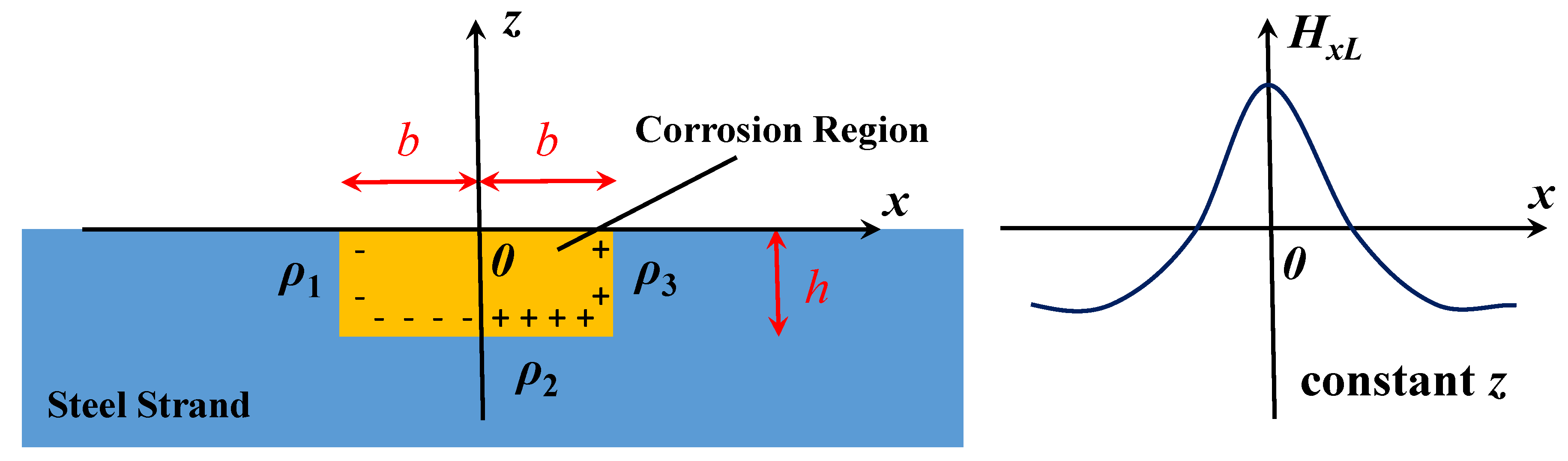
2.1. Magnetic Dipole Model-Based Corrosion Detection Method
2.2. Signal Processing for Extreme Value
3. Experimental Study
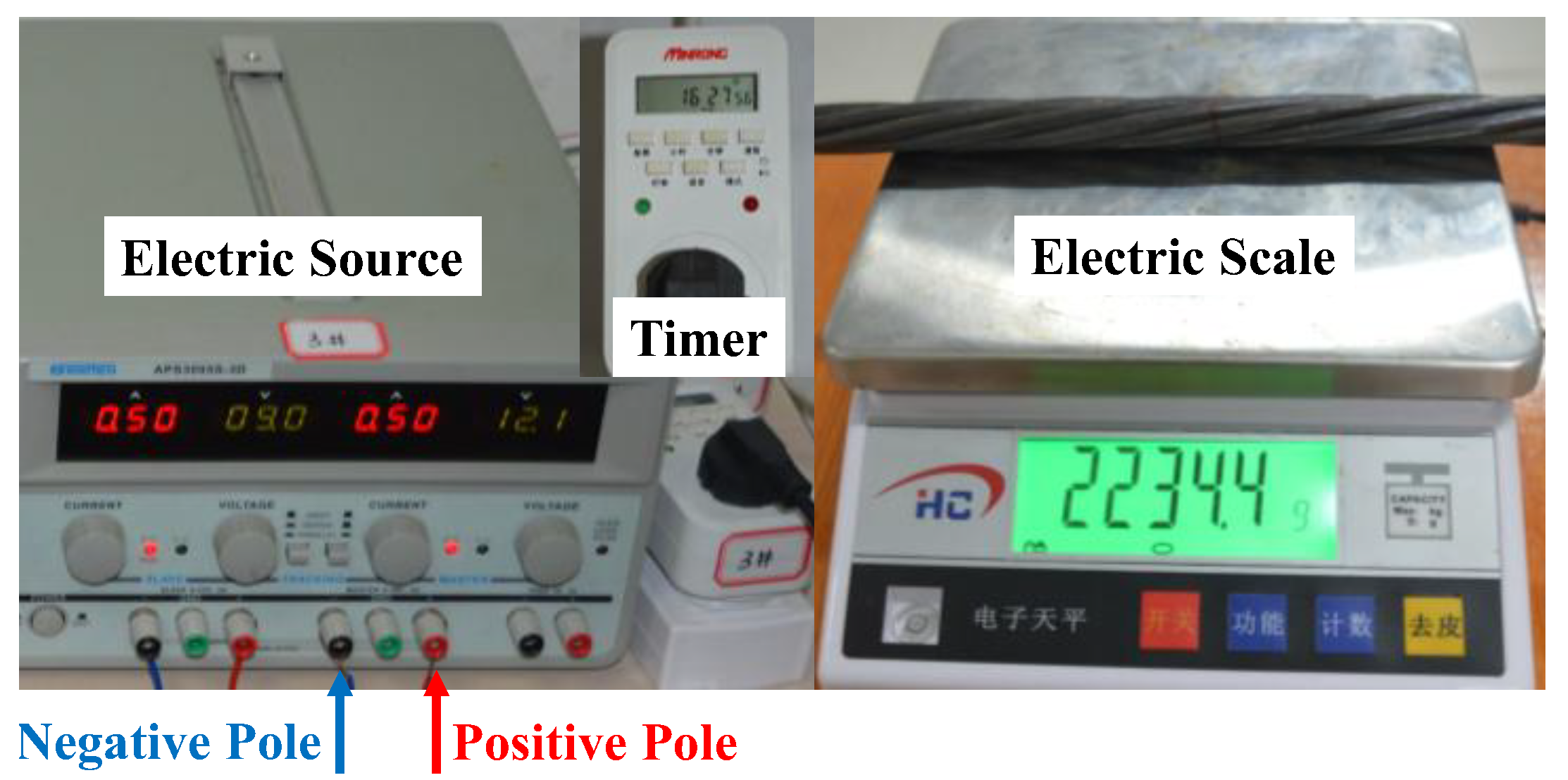
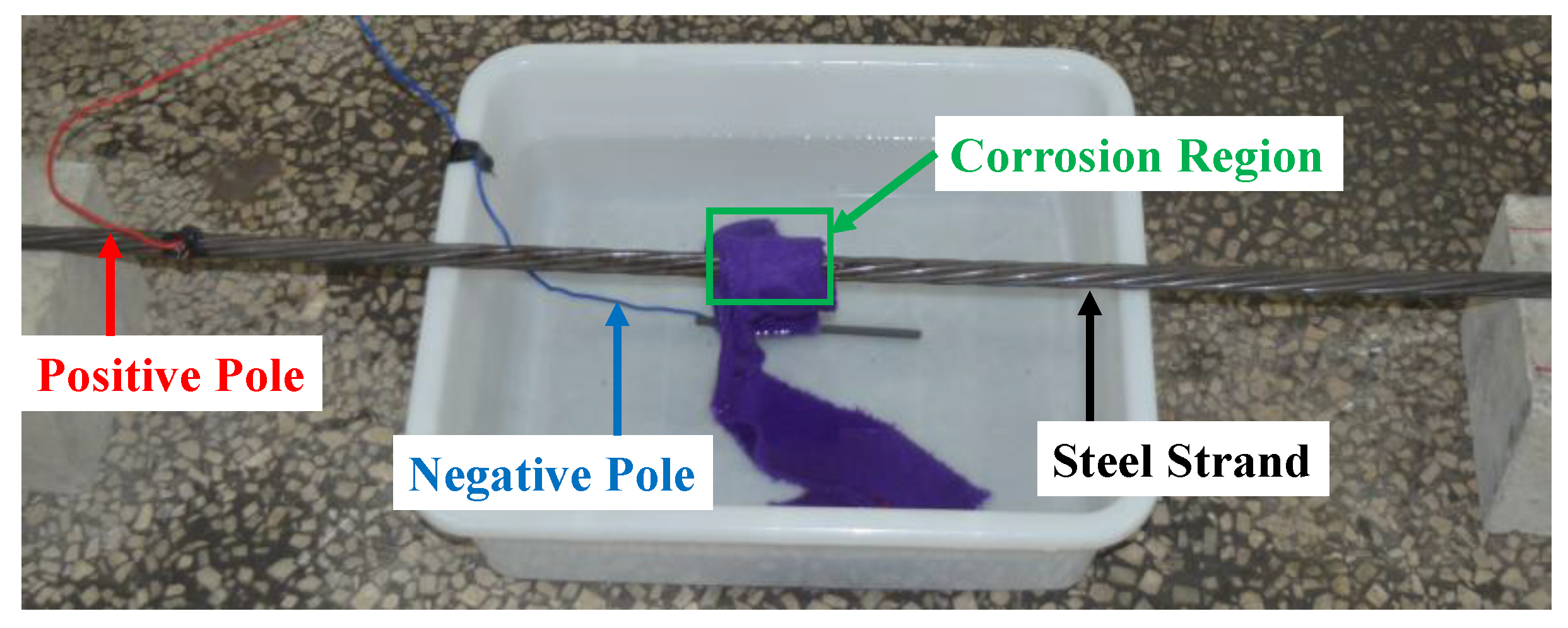
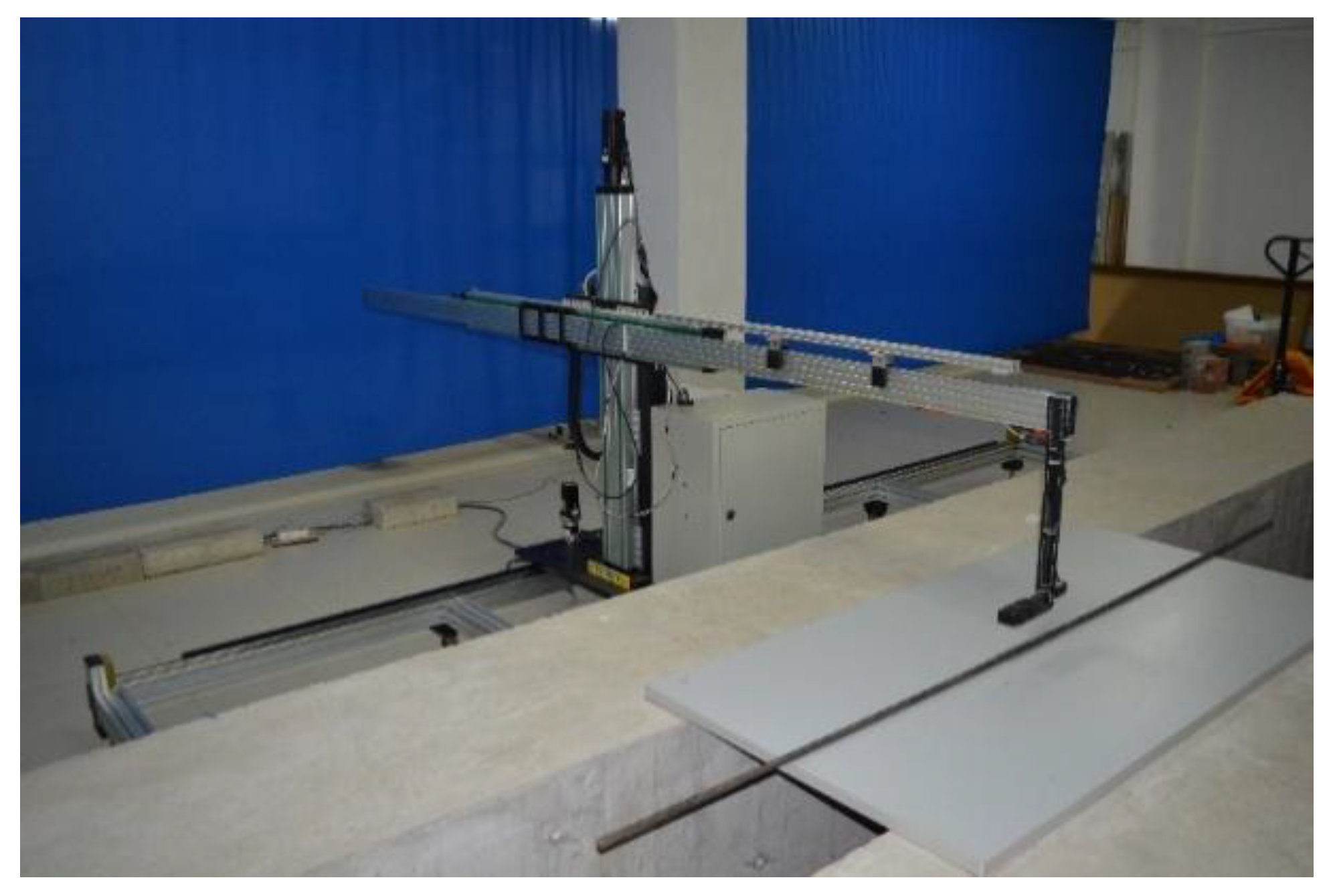
3.1. Experimental Setup and Procedure
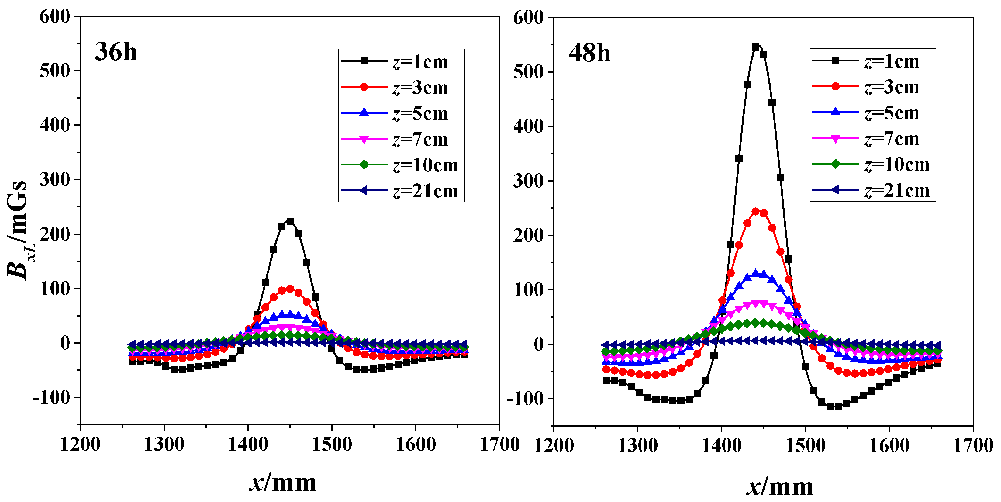
3.2. SMFL Based Corrosion Detection Results
3.3. Quantitative SMFL Signal Analysis Using Magnetic Dipole Model
4. Conclusions
- (1)
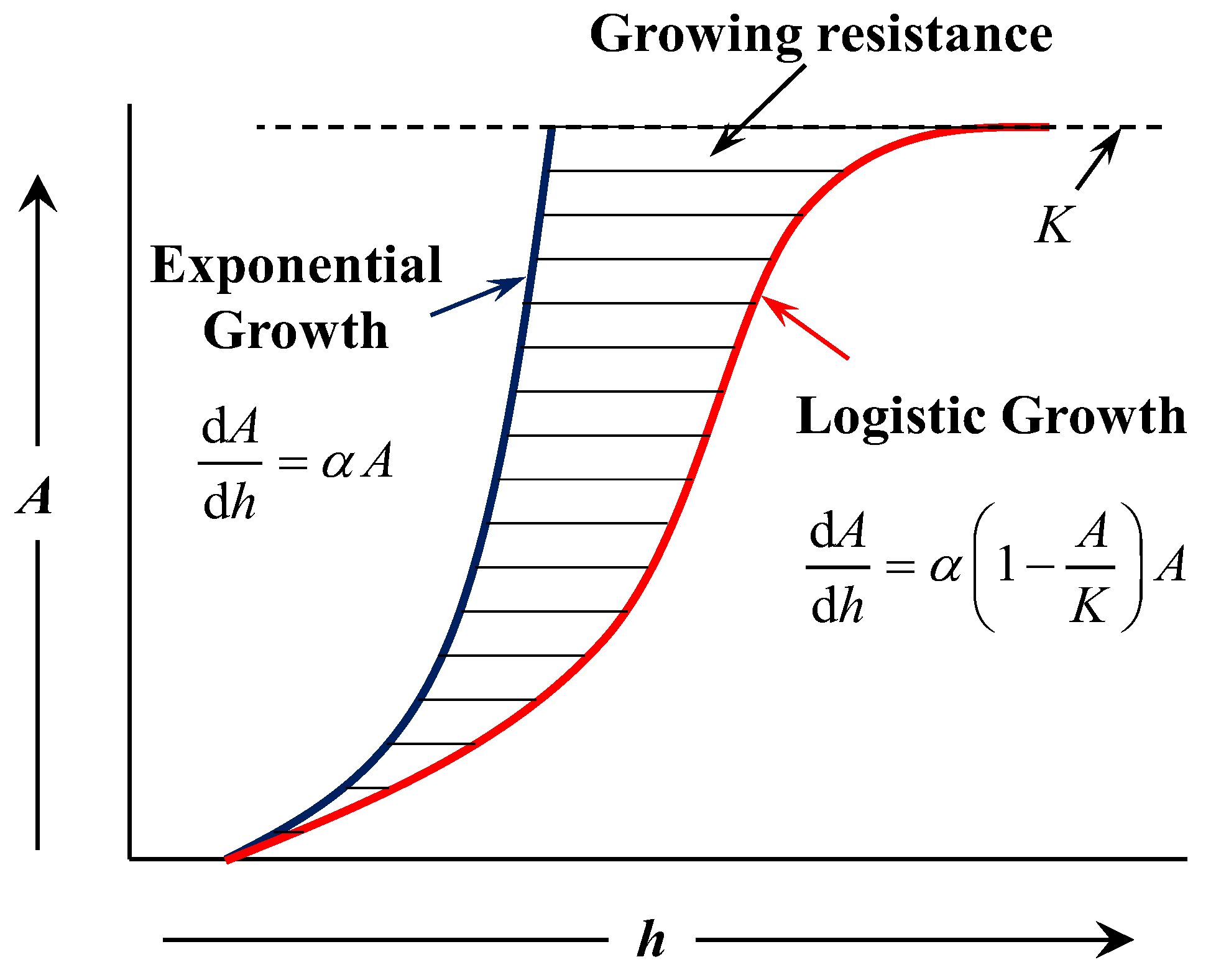
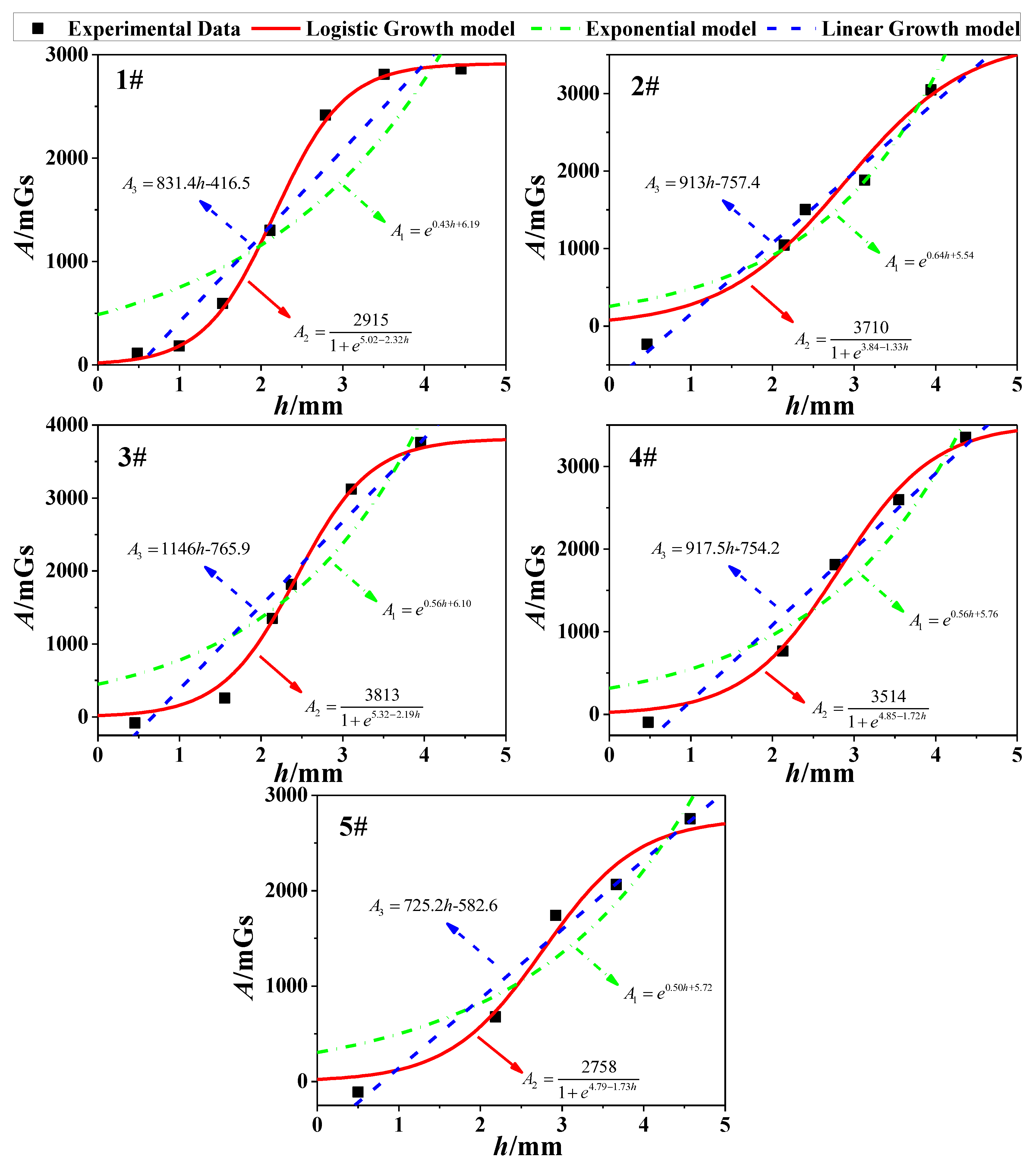
- Combined with the fitting analysis of the experimental data, the Logistic Growth model is in better agreement with the correlation between h and A, and it is verified as the optimal model for calculating the magnetic field (Figure 10).
- (2)
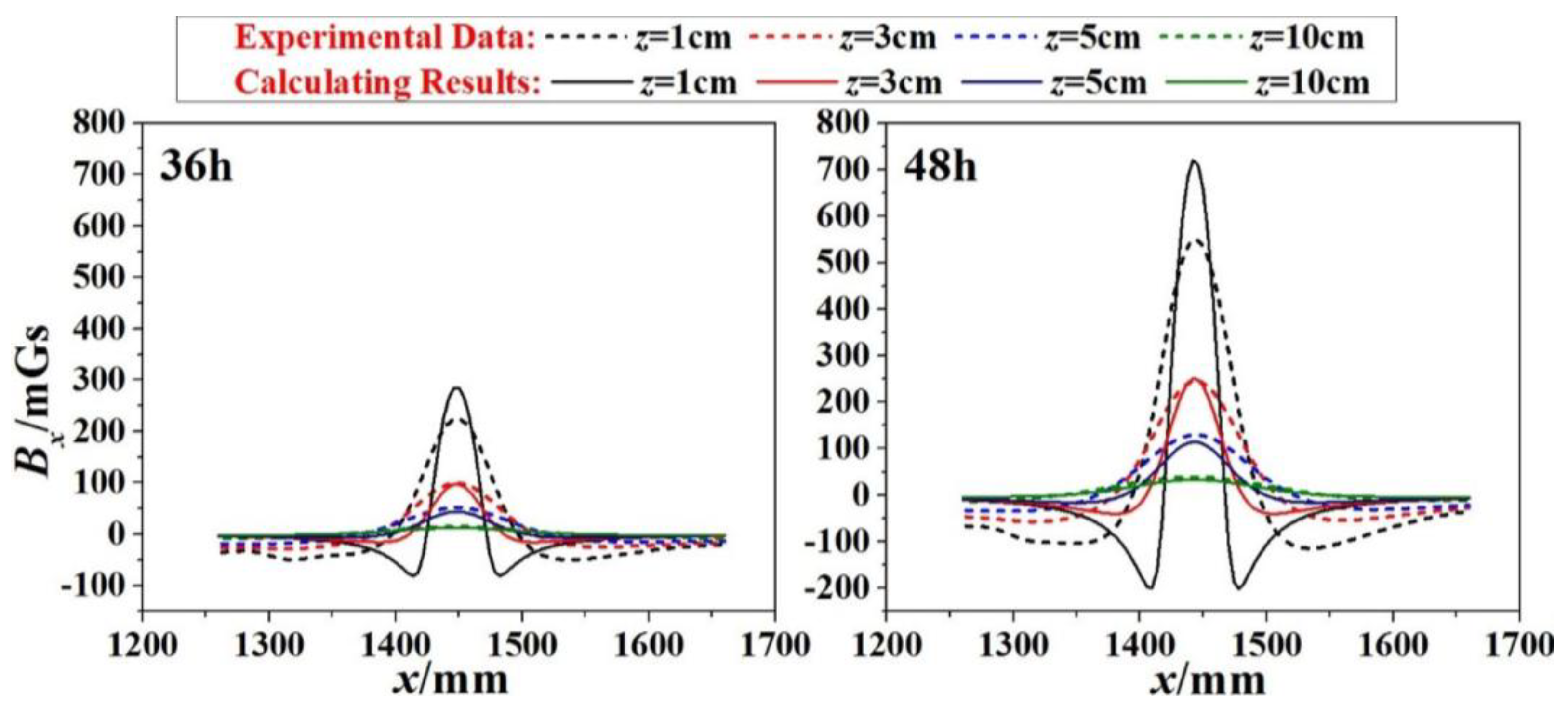
- With the logistic model brought to the original magnetic dipole model, the amplitudes of the calculated values (BxL(x,z) curves) coincide with the measured values in general (Figure 11).
- (3)
- The differences of A for specimens are diverse in the same order of the magnitude. This may be caused by the manufacture of specimens or the material itself, such as the internal twisting force, the different initial defect or the initial magnetization degree.
Author Contributions
Funding
Conflicts of Interest
References
- Capozzoli, L.; Rizzo, E. Combined NDT Techniques in Civil Engineering Applications: Laboratory and the Real Test. Constr. Build. Mater. 2017, 154, 1139–1150. [Google Scholar] [CrossRef]
- Zhang, J.; Liu, C.; Sun, M.; Li, Z. An Innovative Corrosion Evaluation Technique for Reinforced Concrete Structures Using Magnetic Sensors. Constr. Build. Mater. 2017, 135, 68–75. [Google Scholar] [CrossRef]
- Wu, D.; Liu, Z.; Wang, X.; Su, L. Composite Magnetic Flux Leakage Detection Method for Pipelines Using Alternating Magnetic Field Excitation. NDT E Int. 2017, 91, 148–155. [Google Scholar] [CrossRef]
- Nair, A.; Cai, C.S. Acoustic Emission Monitoring of Bridges: Review and Case Studies. Eng. Struct. 2010, 32, 1704–1714. [Google Scholar] [CrossRef]
- Rocío, N.A.M.; Nicolás, N.; Isabel, L.P.M.; José, R.; Linilson, P. Magnetic Barkhausen Noise and Magneto-Acoustic Emission in Stainless Steel Plates. Procedia Mater. Sci. 2015, 8, 674–682. [Google Scholar] [CrossRef]
- Yang, L.J.; Liu, B.; Chen, L.J.; Gao, S.W. The Quantitative Interpretation by Measurement Using The Magnetic Memory Method (MMM)-Based on Density Functional Theory. NDT E Int. 2013, 55, 15–20. [Google Scholar] [CrossRef]
- Huang, H.; Han, G.; Qian, Z.; Liu, Z. Characterizing The Magnetic Memory Signals on The Surface of Plasma Transferred Arc Cladding Coating Under Fatigue Loads. J. Magn. Mater. 2017, 443, 281–296. [Google Scholar] [CrossRef]
- Le, M.; Lee, J.; Jun, J.; Kim, J.; Moh, S.; Shin, K. Hall Sensor Array Based Validation of Estimation of Crack Size in Metals Using Magnetic Dipole Models. NDT E Int. 2013, 53, 18–25. [Google Scholar] [CrossRef]
- Mandache, C.; Clapham, L. A Model for Magnetic Flux Leakage Signal Predictions. J. Phys. D Appl. Phys. 2003, 36, 2427. [Google Scholar] [CrossRef]
- Le, M.; Lee, J.; Shoji, T. A Simulation of Magneto-Optical Eddy Current Imaging. NDT E Int. 2011, 44, 783–788. [Google Scholar] [CrossRef]
- Zhong, W.C. Analysis of Magnetic Leakage Field Caused By a Rectangular Slot on the Workpiece Surface. Nondestruct. Test. 2004, 26, 339–341. [Google Scholar]
- Zhong, W.C. Magnetic Leakage Filed Yielded By a Surface Breaking Discontinuity with Any Shape Transversal Section. Nondestruct. Test. 2006, 28, 633–635. [Google Scholar]
- Shi, P.P. Analytical Solutions of Magnetic Dipole Model for Defect Leakage Magnetic Fields. Nondestruct. Test. 2015, 37, 1–7. [Google Scholar]
- Wang, Z.D.; Yao, K.; Deng, B.; Ding, K.Q. Quantitative Study of Metal Magnetic Memory Signal versus Local Stress Concentration. NDT E Int. 2010, 43, 513–518. [Google Scholar] [CrossRef]
- Zhang, C.Y.; Xiao, C.H.; Gao, J.J. Experiment Research of Magnetic Dipole Model Applicability for a Magnetic Object. J. Basic Sci. Eng. 2010, 18, 862–868. [Google Scholar]
- Tang, J.F.; Gong, S.G.; Wang, J.Y. Two New Magnetic Localization and Parameter Estimation Methods under the Dipole Model. Acta Electron. Sin. 2003, 31, 154–157. [Google Scholar]
- Slim, J.; Gebel, R.; Heberling, D.; Lehrach, A.; Lorentz, B.; Mey, S.; Nass, A.; Rathmann, F.; Reifferscheidt, L. Electromagnetic Simulation and Design of a Novel Waveguide RF Wien Filter for Electric Dipole Moment Measurements of Protons and Deuterons. Nucl. Instrum. Methods Phys. Res. 2016, 828, 116–124. [Google Scholar] [CrossRef]
- Wang, C.Y.; Li, Y.F. The Calculation of Magnetic Field in Magnetic Drivers Based on Equivalent Magnet Charge Theory. J. Changchun Norm. Univ. 2015, 2, 0441. [Google Scholar]
- Zhang, H.; Liao, L.; Zhao, R.Q.; Zhou, J.; Yang, M.; Xia, R. The Non-Destructive Test of Steel Corrosion in Reinforced Concrete Bridges Using a Micro-Magnetic Sensor. Sensors 2016, 16, 1439. [Google Scholar] [CrossRef] [PubMed]
- Forster, F. Nondestructive Inspection by the Method of Magnetic Leakage Fields: Theoretical and Experimental Foundations of the Detection of Surface Cracks of Finite and Infinite Depth. Sov. J. Nondestruct. Test. 1982, 8, 841–859. [Google Scholar]
- Shi, P.P.; Jin, K.; Zheng, X.J. A magnetomechanical model for the magnetic memory method. Int. J. Mech. Sci. 2017, 124, 229–241. [Google Scholar] [CrossRef]
- Han, W.H.; Shen, X.H.; Xu, J.; Wang, P.; Tian, G.Y.; Wu, Z.Y. Fast Estimation of Defect Profiles from the Magnetic Flux Leakage Signal Based on a Multi-Power Affine Projection Algorithm. Sensors 2014, 14, 16454–16466. [Google Scholar] [CrossRef] [PubMed]
- Shi, Y.; Zhang, C.; Li, R.; Cai, M.; Jia, G. Theory and Application of Magnetic Flux Leakage Pipeline Detection. Sensors 2015, 15, 31036–31055. [Google Scholar] [CrossRef] [PubMed]
- Kudryashov, N.A. Logistic Function as a Solution of Many Nonlinear Differential Equations. Appl. Math. Model. 2015, 39, 5733–5742. [Google Scholar] [CrossRef]
- Ji, Y.; Li, Z.P. Logistic Model and Its Application. J. Weifang Univ. 2009, 9, 78–80. [Google Scholar]
- Huy, N.B.; Quan, B.T.; Khanh, N.H. Existence and Multiplicity Results for Generalized Logistic Equations. Nonlinear Anal. Theor. 2016, 144, 77–92. [Google Scholar] [CrossRef]


| Nominal Diameter D/mm | Tensile Strength/MPa | Limit Load Fb/kN | Yield Load Fy/kN |
|---|---|---|---|
| 15.2 | 1860 | 259 | 220 |
| Label | 1# | 2# | 3# | 4# | 5# | |
|---|---|---|---|---|---|---|
| Corrosion Time | ||||||
| 12 h | 6.8 (0.48) | 6.5 (0.46) | 6.4 (0.46) | 6.7 (0.48) | 6.7 (0.48) | |
| 24 h | 13.5 (1.00) | 13.3 (0.98) | 13.2 (0.97) | 13.5 (1.00) | 13.8 (1.02) | |
| 36 h | 19.9 (1.53) | 20.3 (1.56) | 20.2 (1.55) | 20.3 (1.56) | 20.4 (1.57) | |
| 48 h | 26.3 (2.11) | 26.7 (2.15) | 26.6 (2.14) | 26.5 (2.13) | 27.1 (2.18) | |
| 60 h | 33.0 (2.79) | 29.3 (2.40) | 29.0 (2.37) | 32.8 (2.77) | 34.2 (2.92) | |
| 72 h | 39.1 (3.54) | 36.0 (3.13) | 35.8 (3.11) | 39.4 (3.55) | 40.3 (3.67) | |
| 84 h | 45.6 (4.45) | 42.3 (3.94) | 42.4 (3.96) | 45.1 (4.37) | 46.3 (4.57) | |
| Corrosion Time | 12 h | 24 h | 36 h | 48 h | 60 h | 72 h | 84 h | |
|---|---|---|---|---|---|---|---|---|
| z/m | ||||||||
| 0.01 | 41.4 | 69.4 | 222.5 | 548.2 | 1031.8 | 1180.2 | 1204.1 | |
| 0.02 | 26.6 | 45.3 | 145.6 | 356.0 | 671.1 | 793.0 | 827.1 | |
| 0.03 | 18.0 | 30.5 | 99.1 | 245.0 | 467.6 | 557.3 | 586.5 | |
| 0.04 | 12.6 | 21.6 | 70.8 | 174.8 | 338.5 | 410.4 | 436.9 | |
| 0.05 | 9.1 | 15.4 | 51.7 | 129.3 | 252.9 | 310.2 | 332.5 | |
| 0.06 | 6.7 | 11.2 | 39.0 | 98.0 | 193.4 | 240.7 | 259.7 | |
| 0.07 | 5.1 | 8.3 | 29.9 | 76.2 | 151.5 | 190.2 | 206.0 | |
| 0.08 | 3.8 | 6.1 | 23.1 | 60.0 | 120.5 | 152.9 | 166.4 | |
| 0.09 | 2.9 | 4.6 | 18.4 | 48.3 | 97.6 | 124.9 | 136.1 | |
| 0.10 | 2.1 | 3.2 | 14.5 | 39.0 | 79.8 | 103.0 | 112.8 | |
| 0.16 | 0.2 | 0.1 | 4.0 | 13.7 | 29.4 | 39.6 | 43.5 | |
| 0.21 | 0.4 | 0.8 | 1.3 | 6.6 | 15.3 | 21.3 | 22.9 | |
| Corrosion Time | 12 h | 24 h | 36 h | 48 h | 60 h | 72 h | 84 h |
|---|---|---|---|---|---|---|---|
| h/mm | 0.48 | 1.00 | 1.53 | 2.11 | 2.79 | 3.51 | 4.45 |
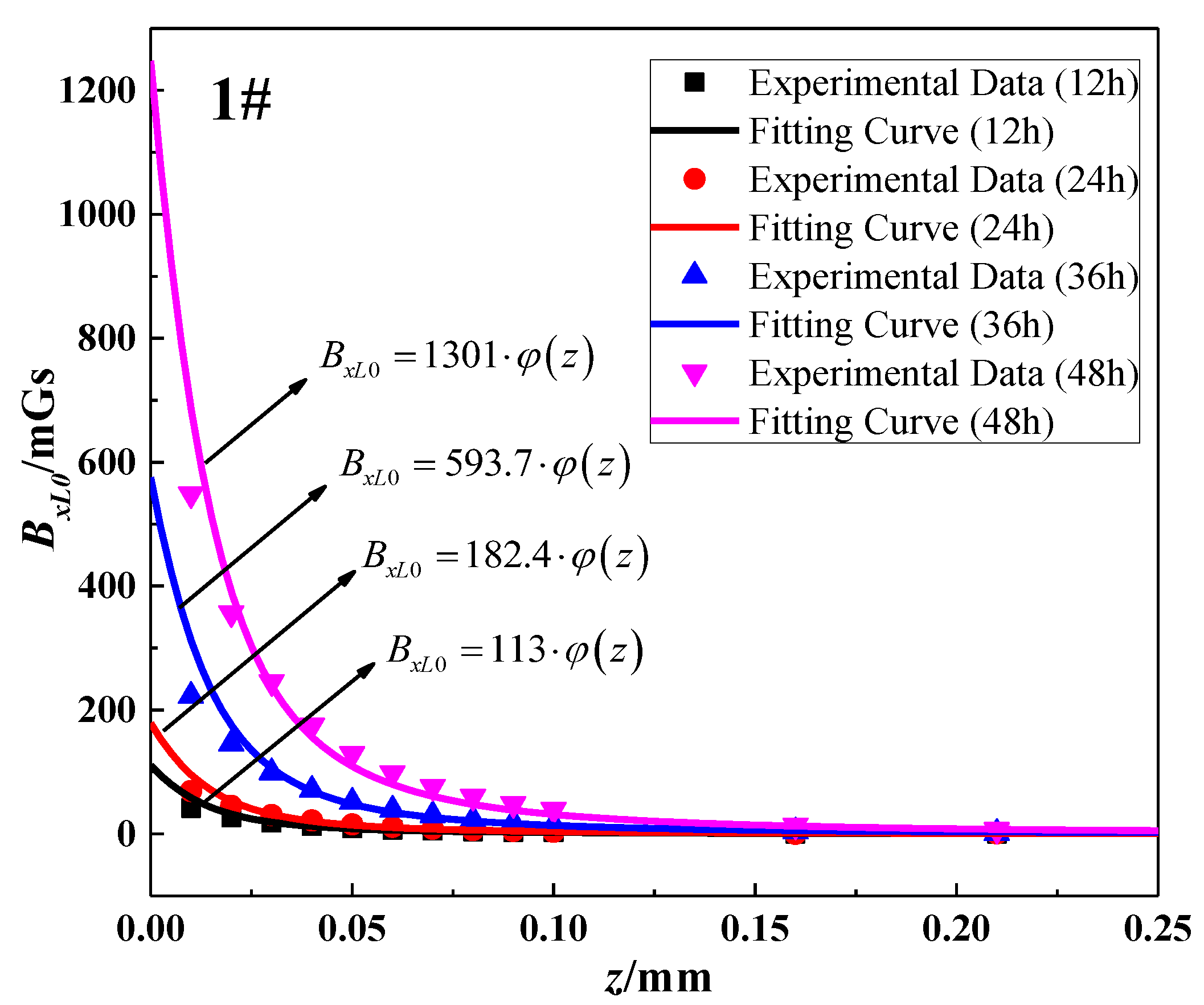
| A | 111.3 | 182.4 | 593.7 | 1301 | 2416 | 2810 | 2864 |
| R2 | 0.9949 | 0.9952 | 0.9942 | 0.9856 | 0.9827 | 0.9771 | 0.9745 |
| 1# | 2# | 3# | 4# | 5# | |
|---|---|---|---|---|---|
| Logistic Growth model | 0.9979 | 0.9527 | 0.9979 | 0.9911 | 0.9766 |
| Exponential Growth model | 0.7894 | 0.9221 | 0.9000 | 0.9215 | 0.8912 |
| Linear Growth model | 0.9245 | 0.9768 | 0.9714 | 0.9666 | 0.9696 |
© 2018 by the authors. Licensee MDPI, Basel, Switzerland. This article is an open access article distributed under the terms and conditions of the Creative Commons Attribution (CC BY) license (http://creativecommons.org/licenses/by/4.0/).
Share and Cite
Xia, R.; Zhou, J.; Zhang, H.; Liao, L.; Zhao, R.; Zhang, Z. Quantitative Study on Corrosion of Steel Strands Based on Self-Magnetic Flux Leakage. Sensors 2018, 18, 1396. https://doi.org/10.3390/s18051396
Xia R, Zhou J, Zhang H, Liao L, Zhao R, Zhang Z. Quantitative Study on Corrosion of Steel Strands Based on Self-Magnetic Flux Leakage. Sensors. 2018; 18(5):1396. https://doi.org/10.3390/s18051396
Chicago/Turabian StyleXia, Runchuan, Jianting Zhou, Hong Zhang, Leng Liao, Ruiqiang Zhao, and Zeyu Zhang. 2018. "Quantitative Study on Corrosion of Steel Strands Based on Self-Magnetic Flux Leakage" Sensors 18, no. 5: 1396. https://doi.org/10.3390/s18051396
APA StyleXia, R., Zhou, J., Zhang, H., Liao, L., Zhao, R., & Zhang, Z. (2018). Quantitative Study on Corrosion of Steel Strands Based on Self-Magnetic Flux Leakage. Sensors, 18(5), 1396. https://doi.org/10.3390/s18051396