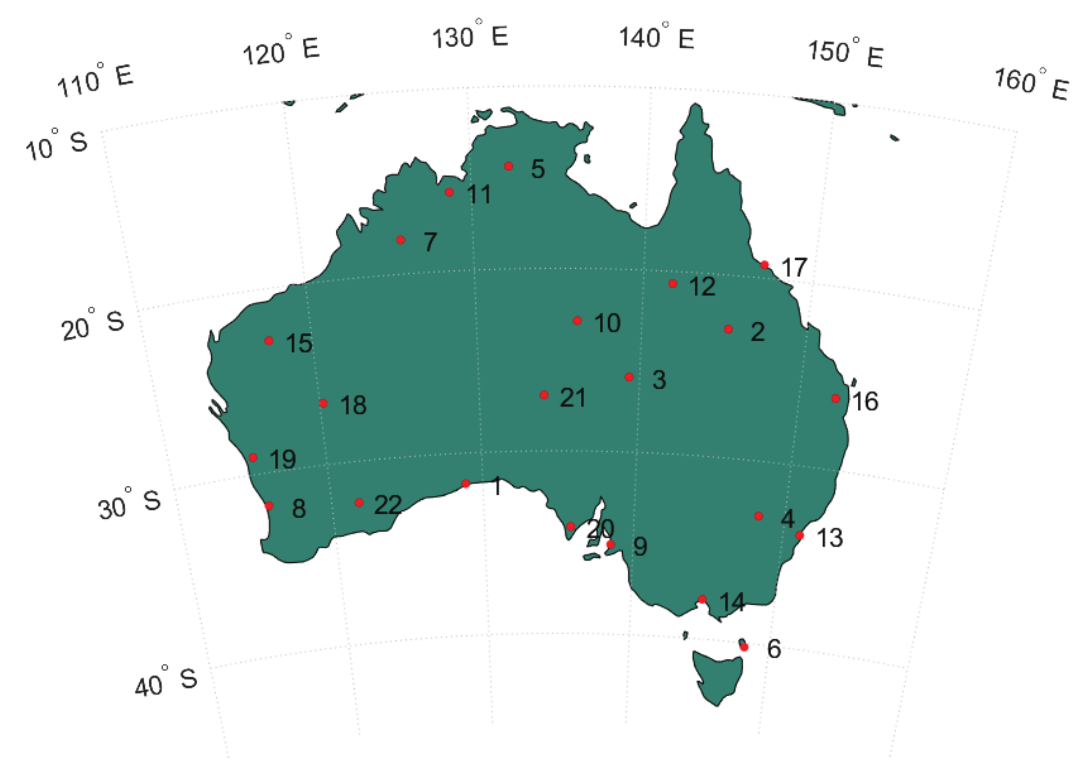
Figure 1.
A network of 22 multi-GNSS continuous operating reference stations (red dots) over Australia. The stations are equipped with various receiver types including Trimble NetR9, Septentrio PolRx5, Septentrio PolaRx4TR, Septentrio PolaRx4TR, Septentrio PolaRxS, and Leica GR30.
Figure 1.
A network of 22 multi-GNSS continuous operating reference stations (red dots) over Australia. The stations are equipped with various receiver types including Trimble NetR9, Septentrio PolRx5, Septentrio PolaRx4TR, Septentrio PolaRx4TR, Septentrio PolaRxS, and Leica GR30.
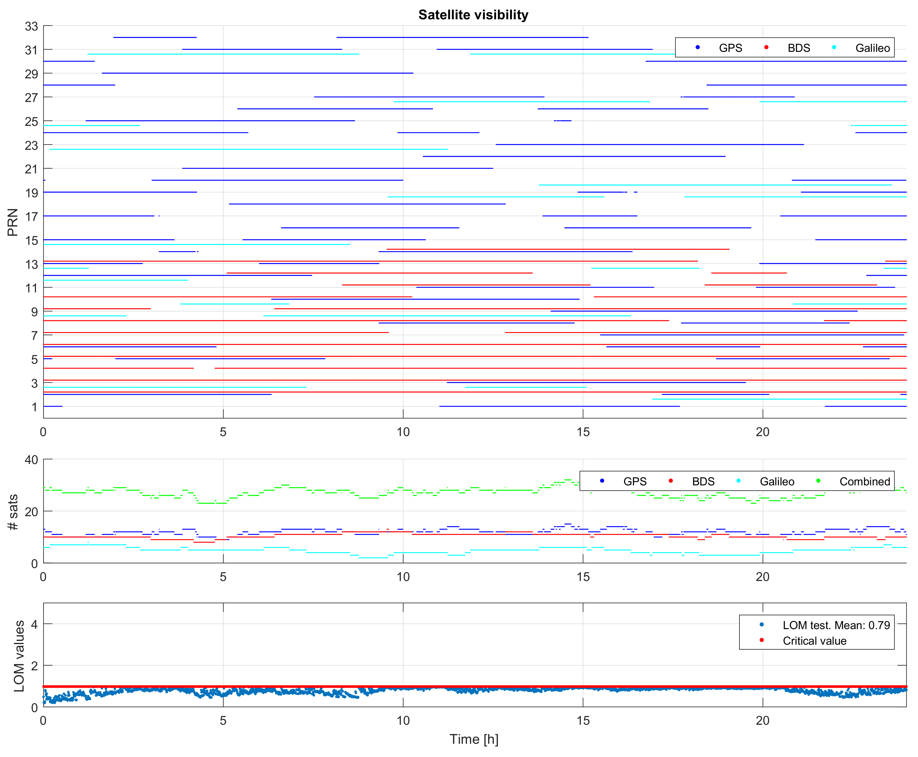
Figure 2.
Satellite visibility, number of satellites, and Local Overall Model (LOM) test outcomes.
Figure 2.
Satellite visibility, number of satellites, and Local Overall Model (LOM) test outcomes.
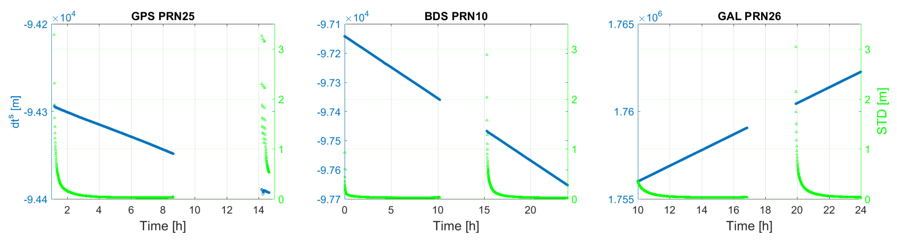
Figure 3.
GPS, BDS, Galileo satellite clock error.
Figure 3.
GPS, BDS, Galileo satellite clock error.
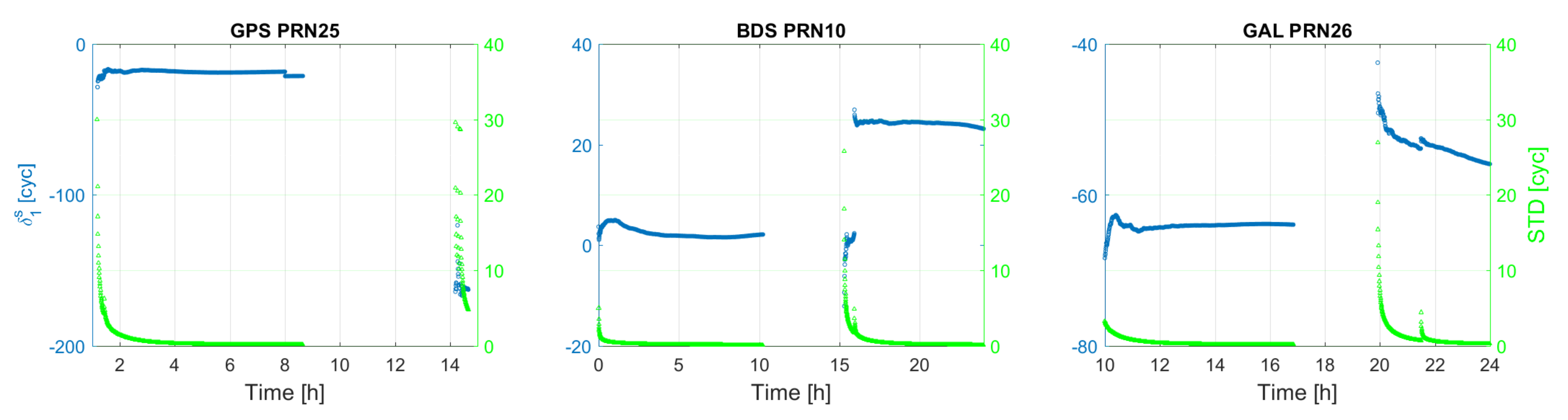
Figure 4.
GPS-L1, BDS-B1, Galileo-E1 satellite phase biases.
Figure 4.
GPS-L1, BDS-B1, Galileo-E1 satellite phase biases.
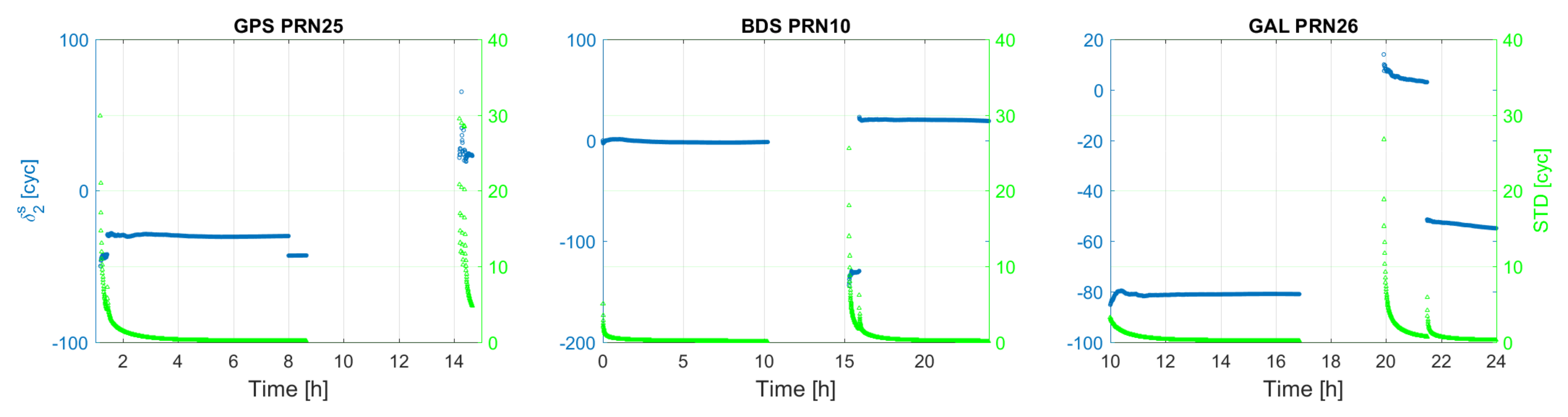
Figure 5.
GPS-L2, BDS-B2, Galileo-E5a satellite phase biases.
Figure 5.
GPS-L2, BDS-B2, Galileo-E5a satellite phase biases.
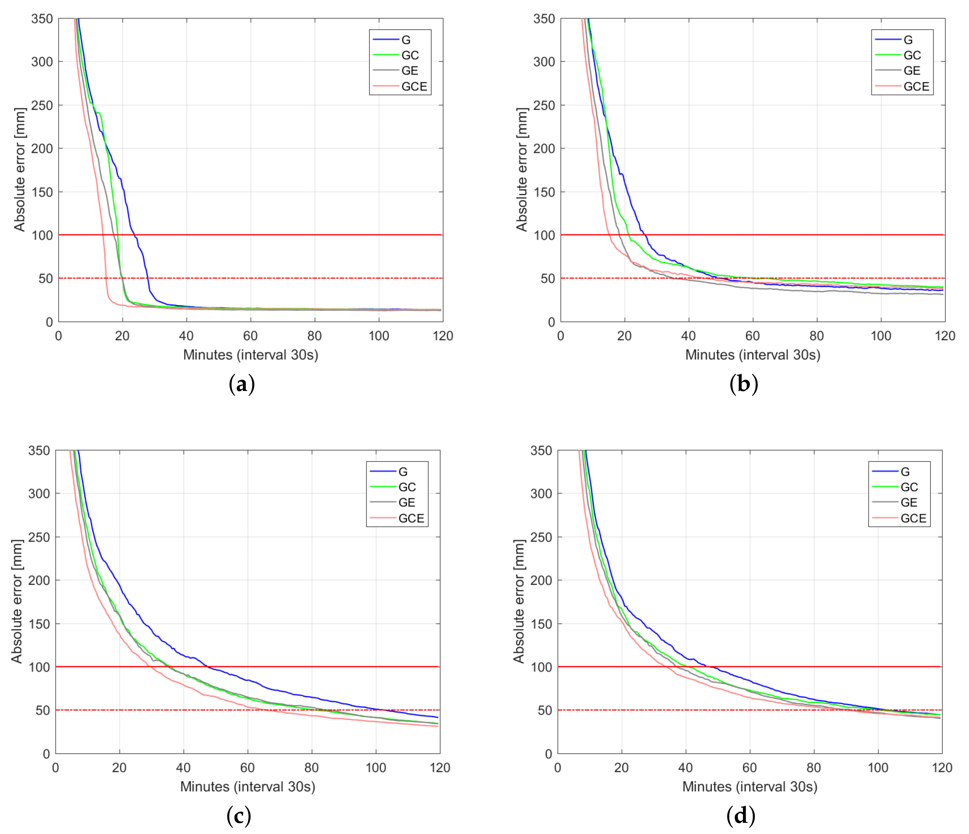
Figure 6.
Convergence behavior (50% of samples) of the horizontal radial position error and up component error based on processing 3800 data windows of multi-GNSS (GPS, BDS, Galileo), dual-frequency (L1-L2, B1-B2, E1-E5a) Australia-wide network data. (a) horizontal radial (fixed); (b) up component (fixed); (c) horizontal radial (float); (d) up component (float).
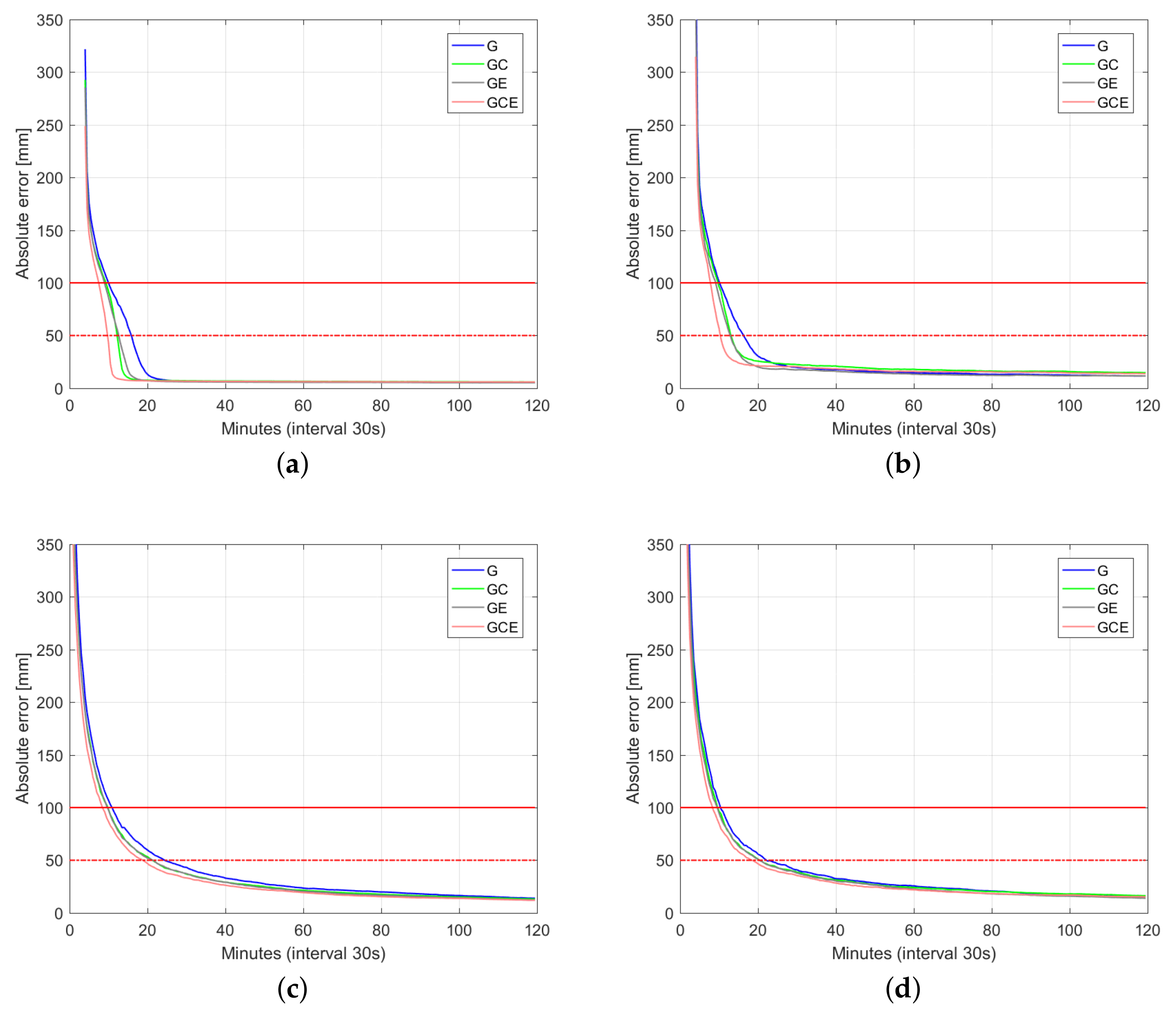
Figure 7.
Convergence behavior (75% of samples) of the horizontal radial position error and up component error based on processing 3800 data windows of multi-GNSS (GPS, BDS, Galileo), dual-frequency (L1-L2, B1-B2, E1-E5a) Australia-wide network data. (a) horizontal radial (fixed); (b) up component (fixed); (c) horizontal radial (float); (d) up component (float).
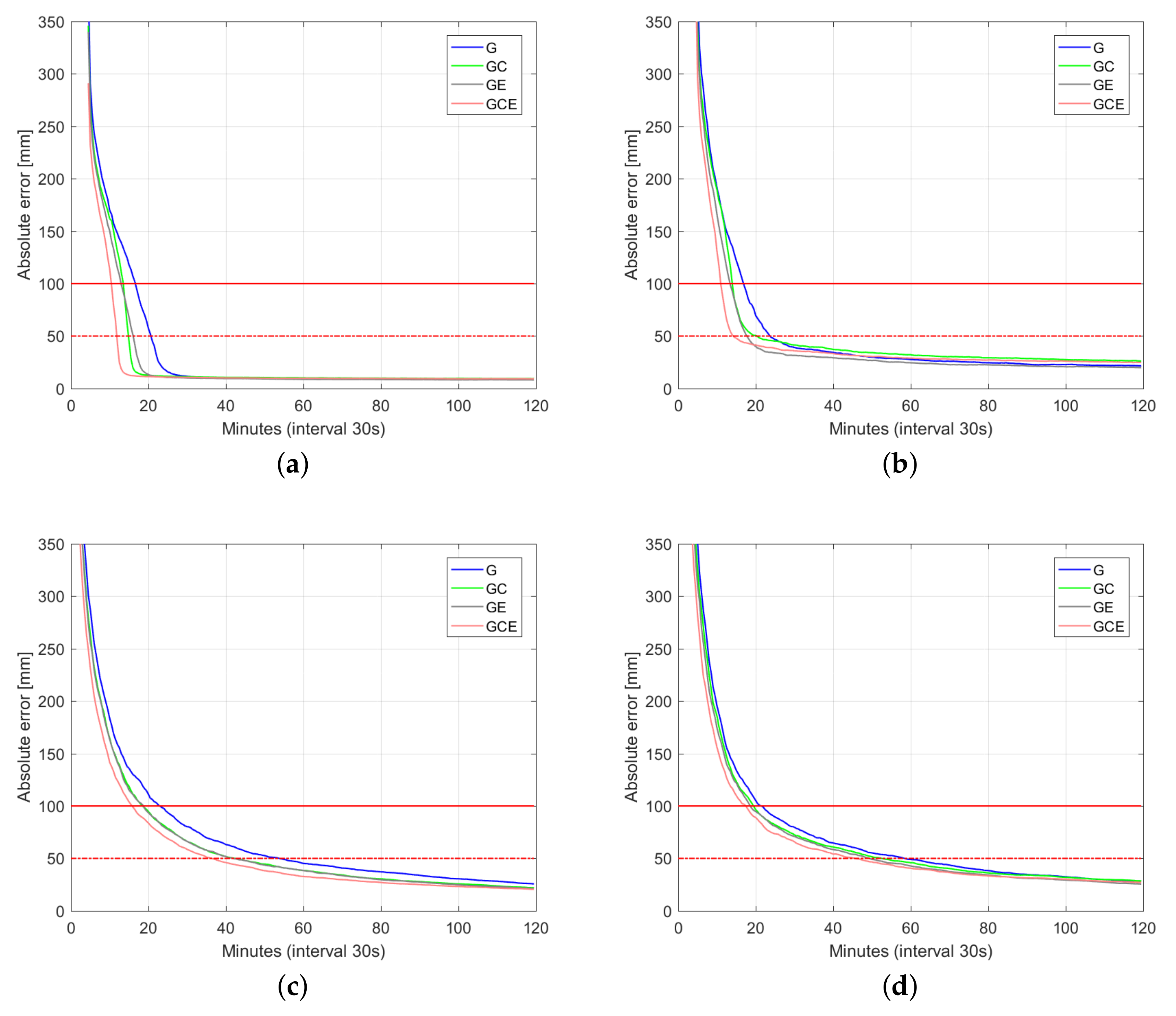
Figure 8.
Convergence behavior (90% of samples) of the horizontal radial position error and up component error based on processing 3800 data windows of multi-GNSS (GPS, BDS, Galileo), dual-frequency (L1-L2, B1-B2, E1-E5a) Australia-wide network data. (a) horizontal radial (fixed); (b) up component (fixed); (c) horizontal radial (float); (d) up component (float).
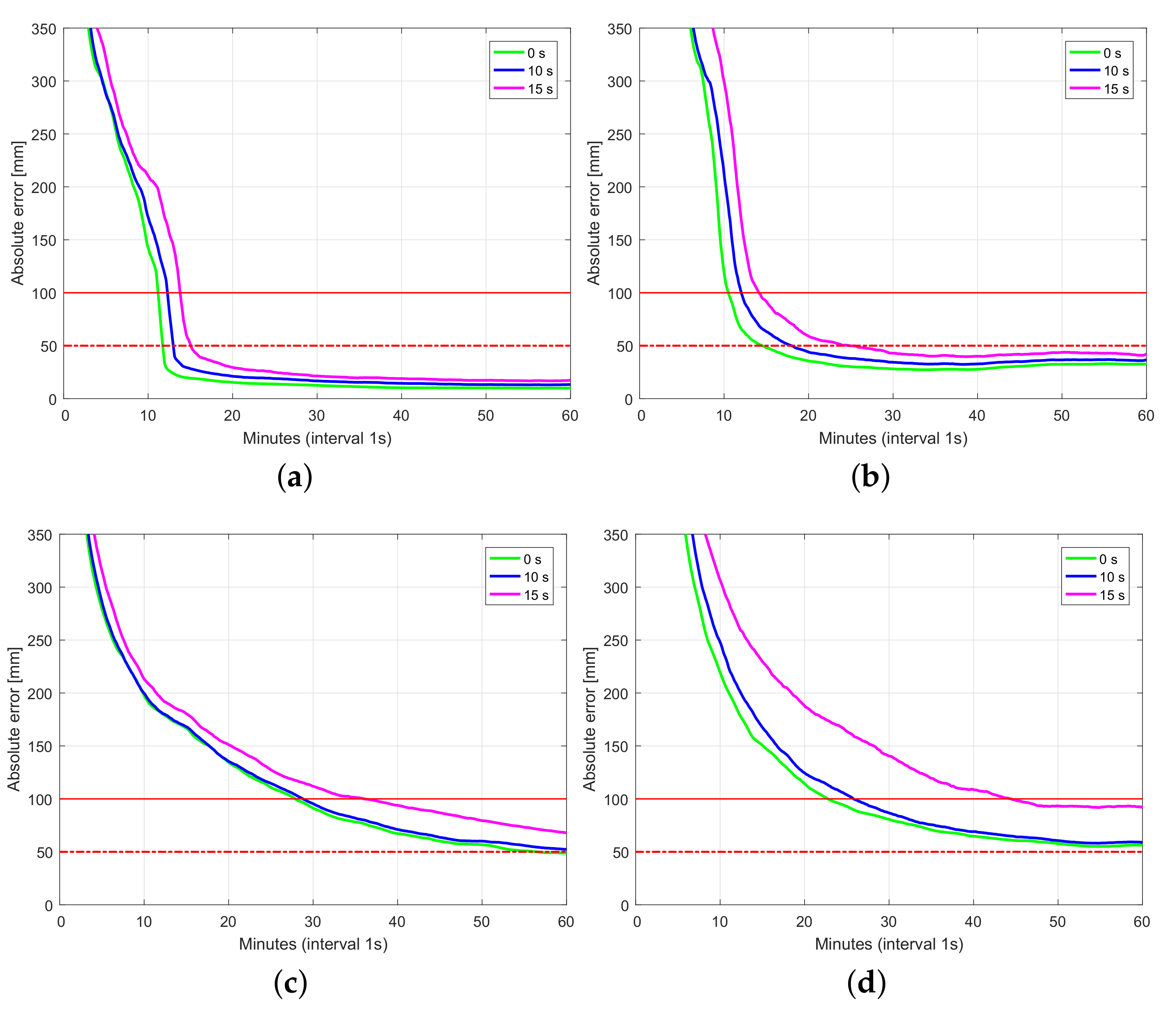
Figure 9.
Convergence behavior (75% of samples) of the horizontal radial position error and up component error in (a,b) ambiguity-fixed and (c,d) -float cases. The network products were estimated without latency (green lines) and predicted with latencies of 10 s (blue lines) and 15 s (magenta lines). 1 Hz GPS dual-frequency data on L1 and L2 were used for the processing. (a) horizontal radial (fixed); (b) up component (fixed); (c) horizontal radial (float); (d) up component (float).
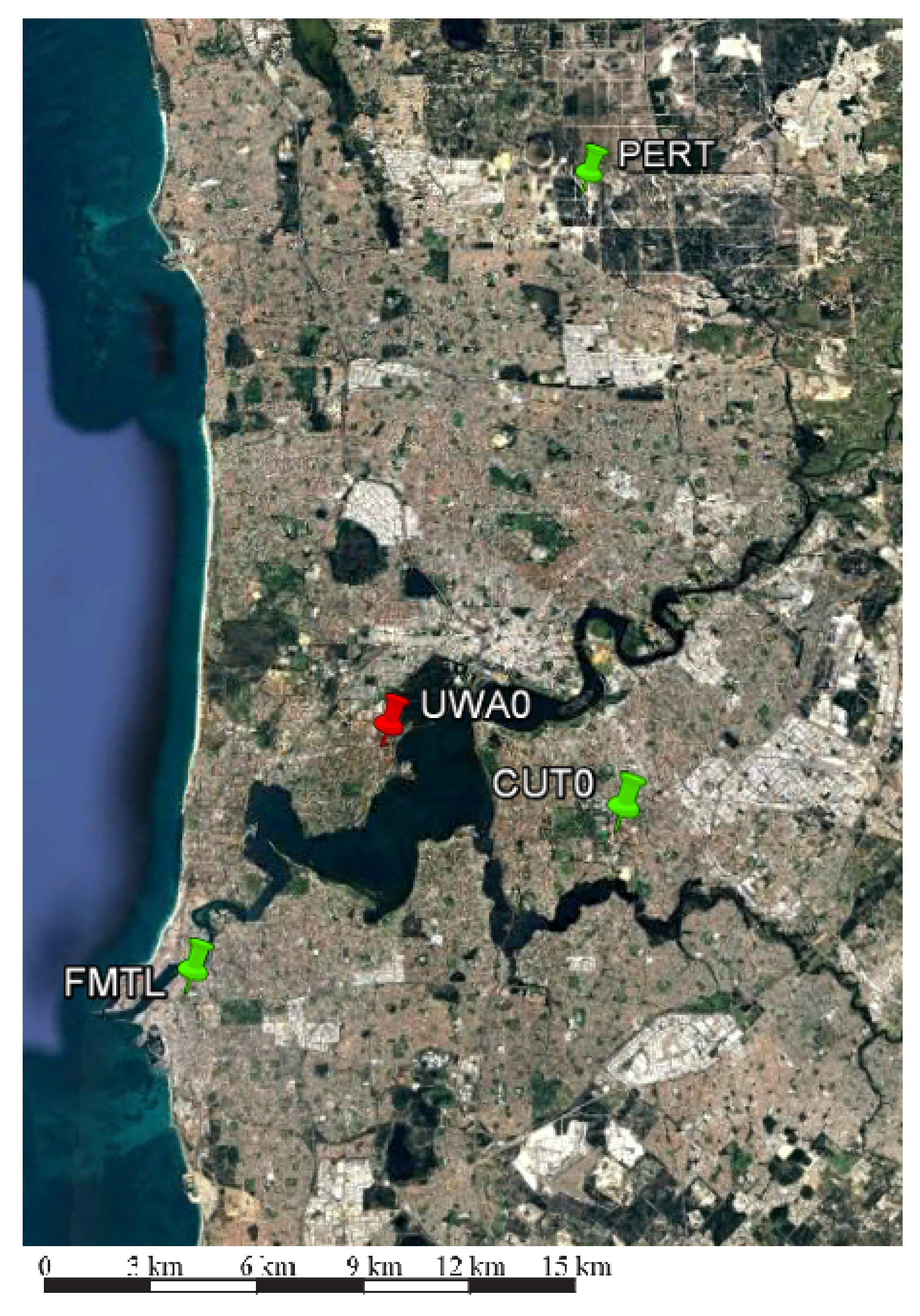
Figure 10.
Multi-GNSS, small-scale network (30 km) (Map data @ 2018 Google, Data SIO, NOAA, U.S. Navy. NGA. GEBCO) [
26].
Figure 10.
Multi-GNSS, small-scale network (30 km) (Map data @ 2018 Google, Data SIO, NOAA, U.S. Navy. NGA. GEBCO) [
26].
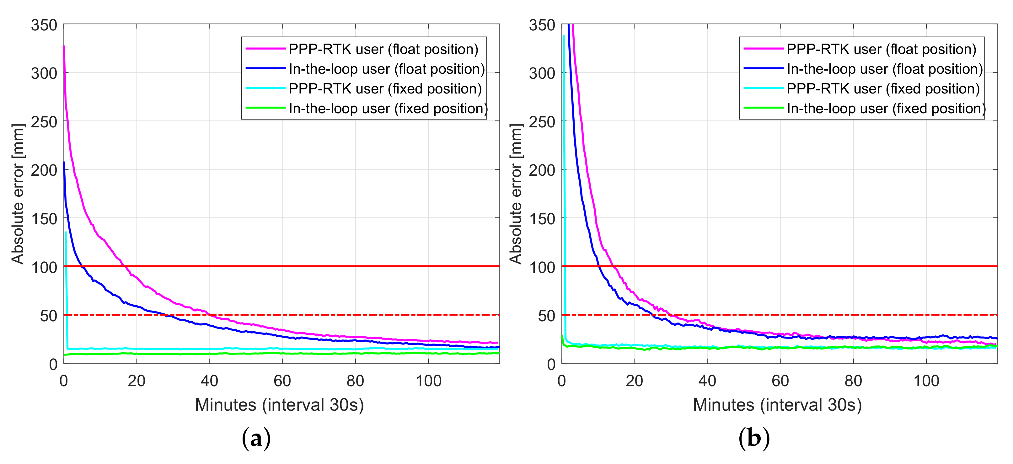
Figure 11.
Convergence behavior (75% of samples) of UWA0 position errors based on processing of 430 data windows of GPS-only dual-frequency (L1-L2) small network data: PPP-RTK user vs. in-loop user. (a) Horizontal radial position error; (b) Up component error.
Figure 11.
Convergence behavior (75% of samples) of UWA0 position errors based on processing of 430 data windows of GPS-only dual-frequency (L1-L2) small network data: PPP-RTK user vs. in-loop user. (a) Horizontal radial position error; (b) Up component error.
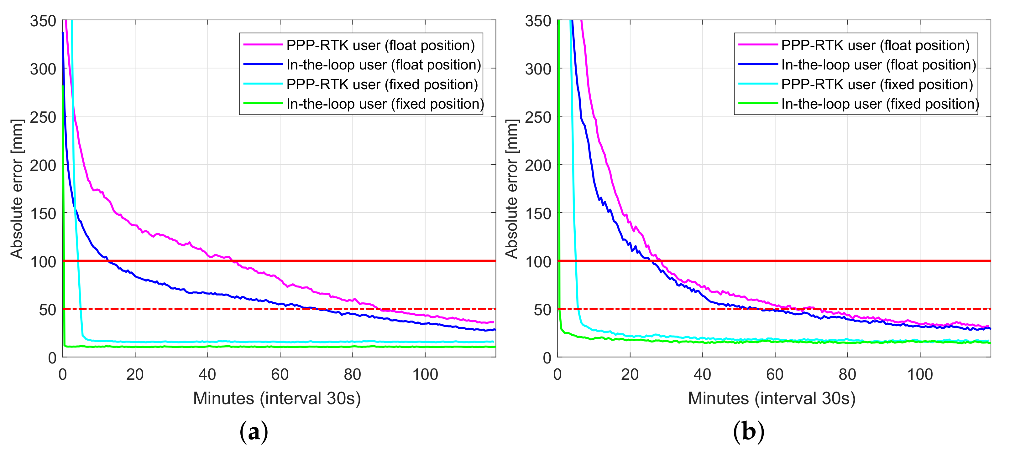
Figure 12.
Convergence behavior (75% of samples) of UWA0 position errors based on processing of 430 data windows of multi-GNSS (GPS, BDS, Galileo), dual-frequency (L1-L2, B1-B2, E1-E5a) small network data: PPP-RTK user vs. in-loop user. (a) horizontal radial position error; (b) up component error.
Figure 12.
Convergence behavior (75% of samples) of UWA0 position errors based on processing of 430 data windows of multi-GNSS (GPS, BDS, Galileo), dual-frequency (L1-L2, B1-B2, E1-E5a) small network data: PPP-RTK user vs. in-loop user. (a) horizontal radial position error; (b) up component error.
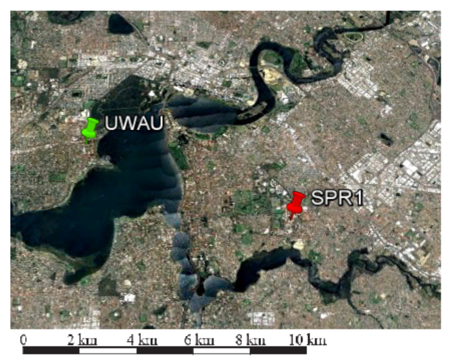
Figure 13.
Multi-GNSS, single-frequency low-cost network (7 km) (Map data @ 2018 Google, Data SIO, NOAA, U.S. Navy. NGA. GEBCO) [
26].
Figure 13.
Multi-GNSS, single-frequency low-cost network (7 km) (Map data @ 2018 Google, Data SIO, NOAA, U.S. Navy. NGA. GEBCO) [
26].
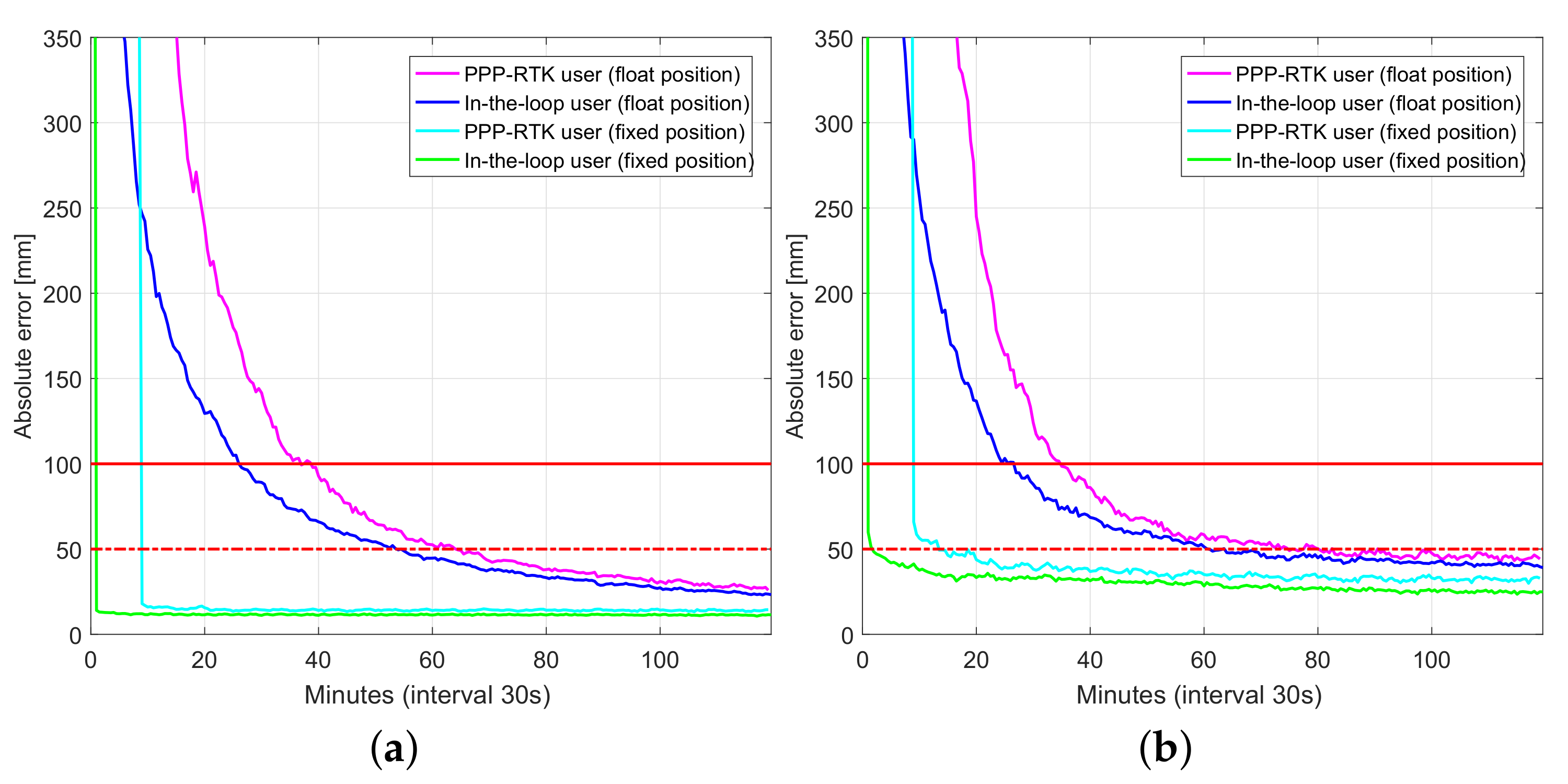
Figure 14.
Convergence behavior (75% of samples) of SPR1 position errors based on processing of 356 data windows of multi-GNSS (GPS, BDS, Galileo), single-frequency (L1, B1, E1) low-cost network data: PPP-RTK user vs. in-loop user. (a) horizontal radial position error; (b) up component error.
Figure 14.
Convergence behavior (75% of samples) of SPR1 position errors based on processing of 356 data windows of multi-GNSS (GPS, BDS, Galileo), single-frequency (L1, B1, E1) low-cost network data: PPP-RTK user vs. in-loop user. (a) horizontal radial position error; (b) up component error.
Table 1.
Estimable GNSS (Global Navigation Satellite System) network-derived parameters formed by an
-basis [
16]. The additional parameters
and
(within
) are taken as
-basis for the small-to-regional scale networks, i.e., when
and
(
). The argument
stands for the epoch index.
Table 1.
Estimable GNSS (Global Navigation Satellite System) network-derived parameters formed by an
-basis [
16]. The additional parameters
and
(within
) are taken as
-basis for the small-to-regional scale networks, i.e., when
and
(
). The argument
stands for the epoch index.
| Position increments | |
| ZTDs (Zenith Tropospheric Delays) | |
| Ionospheric delays | |
| Satellite clocks | |
| Receiver clocks | |
| Sat. phase biases | |
| Rec. phase biases | |
| Sat. code biases | |
| Rec. code biases | |
| Ambiguities | |
| -basis parameters | |
Table 2.
Parameter settings for Australia-wide network processing.
Table 2.
Parameter settings for Australia-wide network processing.
| Stochastic Model with Sinusoidal Elevation Dependent Function |
| Zenith phase noise standard deviation | 3 mm |
| Zenith code noise standard deviation | 30 cm |
| Elevation weighting | Sine function |
| Elevation cut-off | 10 |
| Dynamic Model |
| Ambiguities | Time-constant |
| Satellite biases | Time-constant |
| Receiver biases | Time-constant |
| Troposphere delays (Random-walk) | |
| Ionosphere delays | Unlinked in time |
| Satellite clocks | Unlinked in time |
| Receiver clocks | Unlinked in time |
| Ambiguity Resolution |
| Ambiguity resolution | Partial fixing |
| Expected minimum success rate () | 0.999 |
| Fixing BDS Geostationary satellite ambiguities | No |
| Ionosphere |
| Ionosphere spatial model | None (Ionosphere float) |
Table 3.
(50%) Convergence time of user estimates to 1 dm (in brackets 5 cm) with respect to ground truth.
Table 3.
(50%) Convergence time of user estimates to 1 dm (in brackets 5 cm) with respect to ground truth.
| System | Fixed (min) | Float (min) |
|---|
| Horizontal | Up | Horizontal | Up |
|---|
| GPS | 10.0 (16.0) | 10.0 (16.5) | 11.0 (25.0) | 10.5 (22.5) |
| GPS + BDS | 9.5 (12.5) | 9.5 (13.0) | 10.0 (21.5) | 9.5 (20.5) |
| GPS + Galileo | 9.0 (12.5) | 9.0 (10.5) | 10.0 (21.5) | 9.5 (20.5) |
| GPS + BDS + Galileo | 7.5 (10.0) | 8.0 (10.5) | 8.5 (19.0) | 8.5 (18.5) |
Table 4.
(75%) Convergence time of user estimates to 1 dm (in brackets 5 cm) with respect to ground truth.
Table 4.
(75%) Convergence time of user estimates to 1 dm (in brackets 5 cm) with respect to ground truth.
| System | Fixed (min) | Float (min) |
|---|
| Horizontal | Up | Horizontal | Up |
|---|
| GPS | 16.5 (20.5) | 17.0 (23.5) | 23.0 (53.5) | 21.5 (57.5) |
| GPS + BDS | 13.5 (15.0) | 14.0 (20.0) | 18.5 (42.0) | 19.5 (52.5) |
| GPS + Galileo | 13.0 (16.0) | 13.5 (17.5) | 18.5 (42.0) | 18.5 (49.5) |
| GPS + BDS + Galileo | 10.5 (12.0) | 11.0 (14.0) | 16.0 (36.5) | 17.5 (46.0) |
Table 5.
(90%) Convergence time of user estimates to 1 dm (in brackets 5 cm) with respect to ground truth.
Table 5.
(90%) Convergence time of user estimates to 1 dm (in brackets 5 cm) with respect to ground truth.
| System | Fixed (min) | Float (min) |
|---|
| Horizontal | Up | Horizontal | Up |
|---|
| GPS | 23.5 (28.0) | 26.5 (49.5) | 47.5 (102.5) | 47.5 (102.5) |
| GPS + BDS | 18.5 (20.0) | 21.5 (59.5) | 36.0 (81.0) | 40.5 (100.5) |
| GPS + Galileo | 17.5 (20.0) | 18.5 (35.0) | 35.0 (85.0) | 37.0 (91.5) |
| GPS + BDS + Galileo | 14.0 (15.0) | 15.5 (44.5) | 30.0 (65.5) | 33.5 (89.5) |
Table 6.
Parameter settings for Australia-wide network processing with satellite clock model; Other parameter settings are as in
Table 2.
Table 6.
Parameter settings for Australia-wide network processing with satellite clock model; Other parameter settings are as in
Table 2.
| Dynamic Model |
|---|
| Satellite clocks | = 0.001 m/ |
Table 7.
Parameter settings for small network processing; Other parameter settings are as in
Table 2.
Table 7.
Parameter settings for small network processing; Other parameter settings are as in
Table 2.
| Ionosphere |
|---|
| Ionosphere spatial model | Ionosphere weighted |
| Applicable inter-station distance () | 2 km |
| Standard deviation of undifference ionosphere observables | 0.01 m/ |
Table 8.
(75%) Convergence time of user coordinate estimates to 1 dm (in brackets 5 cm) using GPS-only data of the small-scale network (ionosphere-weighted model).
Table 8.
(75%) Convergence time of user coordinate estimates to 1 dm (in brackets 5 cm) using GPS-only data of the small-scale network (ionosphere-weighted model).
| Method | Fixed (min) | Float (min) |
|---|
| Horizontal | Up | Horizontal | Up |
|---|
| PPP-RTK user | 4.5 (5.0) | 5.0 (5.5) | 47.0 (87.0) | 28.5 (64.5) |
| In-the-loop user | 0.5 (0.5) | 0.5 (0.5) | 12.5 (70.0) | 25.5 (55.5) |
Table 9.
(75%) Convergence time of user coordinate estimates to 1 dm (in brackets 5 cm) using multi-GNSS data of the small-scale network (ionosphere-weighted model).
Table 9.
(75%) Convergence time of user coordinate estimates to 1 dm (in brackets 5 cm) using multi-GNSS data of the small-scale network (ionosphere-weighted model).
| Method | Fixed (min) | Float (min) |
|---|
| Horizontal | Up | Horizontal | Up |
|---|
| PPP-RTK user | 1.0 (1.0) | 0.5 (0.5) | 17.0 (40.5) | 14.0 (30.0) |
| In-the-loop user | 0.0 (0.0) | 0.0 (0.0) | 5.0 (27.5) | 10.5 (25.0) |
Table 10.
Parameter settings for low-cost network processing; other parameters are as in
Table 2.
Table 10.
Parameter settings for low-cost network processing; other parameters are as in
Table 2.
| Stochastic Model with Sinusoidal Elevation Dependent Function |
| Zenith phase noise standard deviation | GPS: 3 mm, BDS: 4 mm, Galileo: 3 mm |
| Zenith code noise standard deviation | GPS: 60 cm, BDS: 80 cm, Galileo: 60 cm |
| Dynamic Model |
| Receiver biases | Unlinked in time |
| Ionosphere |
| Ionosphere spatial model | Ionosphere weighted |
| Applicable inter-station distance () | 2 km |
| Standard deviation of undifference ionosphere observables | 0.1 m/ |
Table 11.
(75%) Convergence time of user coordinate estimates to 1 dm (in brackets 5 cm) using low-cost multi-GNSS receivers (ionosphere-weighted model).
Table 11.
(75%) Convergence time of user coordinate estimates to 1 dm (in brackets 5 cm) using low-cost multi-GNSS receivers (ionosphere-weighted model).
| Method | Fixed (min) | Float (min) |
|---|
| Horizontal | Up | Horizontal | Up |
|---|
| PPP-RTK user | 9.0 (9.0) | 9.0 (13.5) | 39.0 (64.5) | 35.5 (75.0) |
| In-the-loop user | 1.0 (1.0) | 1.0 (2.0) | 26.0 (54.0) | 27.0 (61.0) |

 ,
, 


