Automatic Modulation Classification Based on Deep Learning for Unmanned Aerial Vehicles

 ,
, 
Abstract
:1. Introduction
- (1)
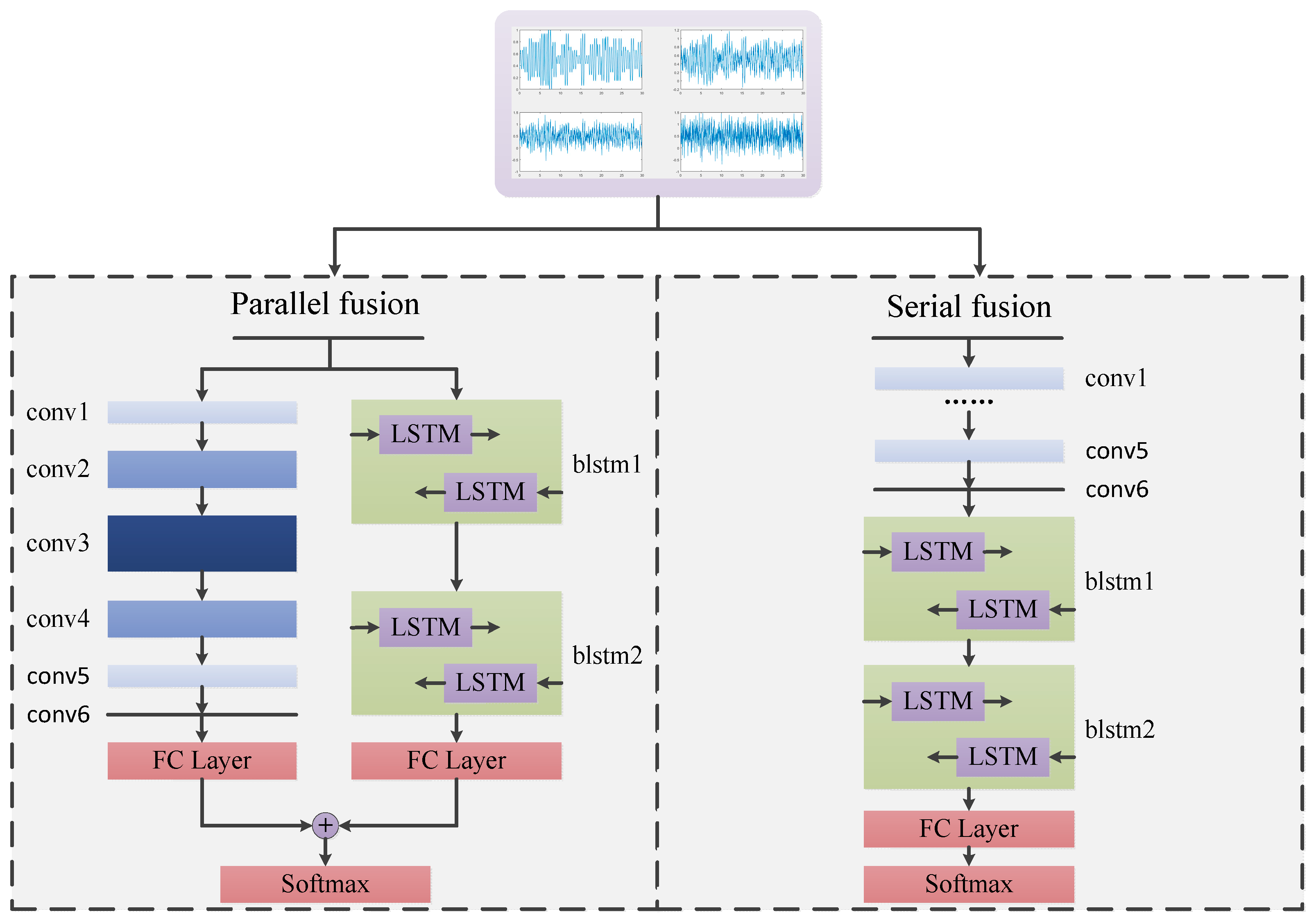
- CNNs and LSTM are fused based on the serial and parallel modes to solve the AMC problem, thereby leading to two HDMFs. Both are trained in the end-to-end framework, which can learn features and make classifications in a unified framework.
- (2)
- The experimental results show that the performance of the fusion model is significantly improved compared with the independent network and also with traditional wavelet/SVM models. The serial version of HDMF achieves much better performance than the parallel version.
- (3)
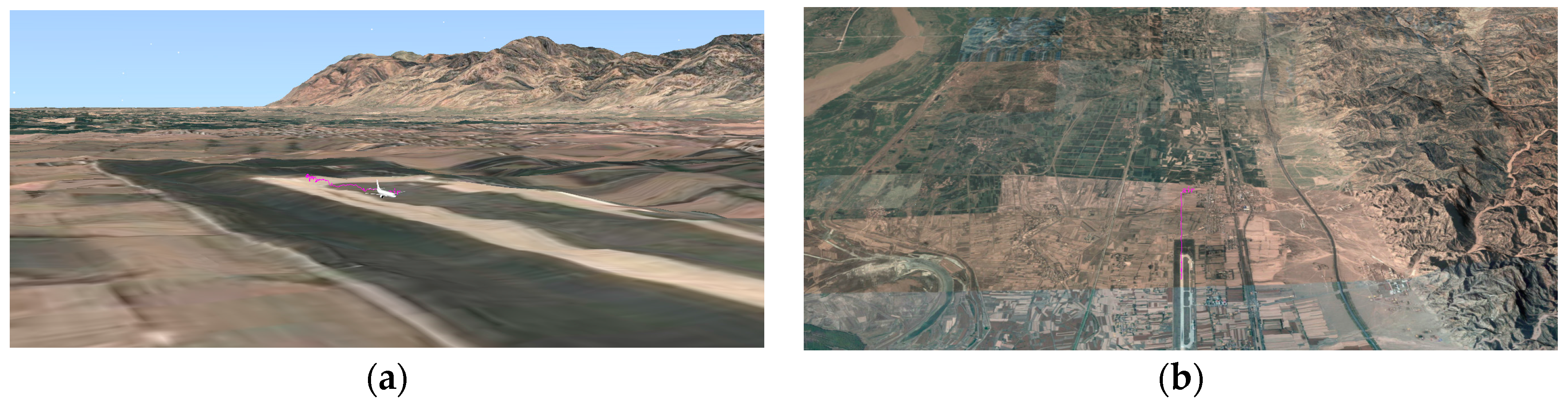
- We collect communication signal data sets which approximate the transmitted wireless channel in an actual geographical environment. Such datasets are very useful for training networks like CNNs and LSTM.
2. Related Works
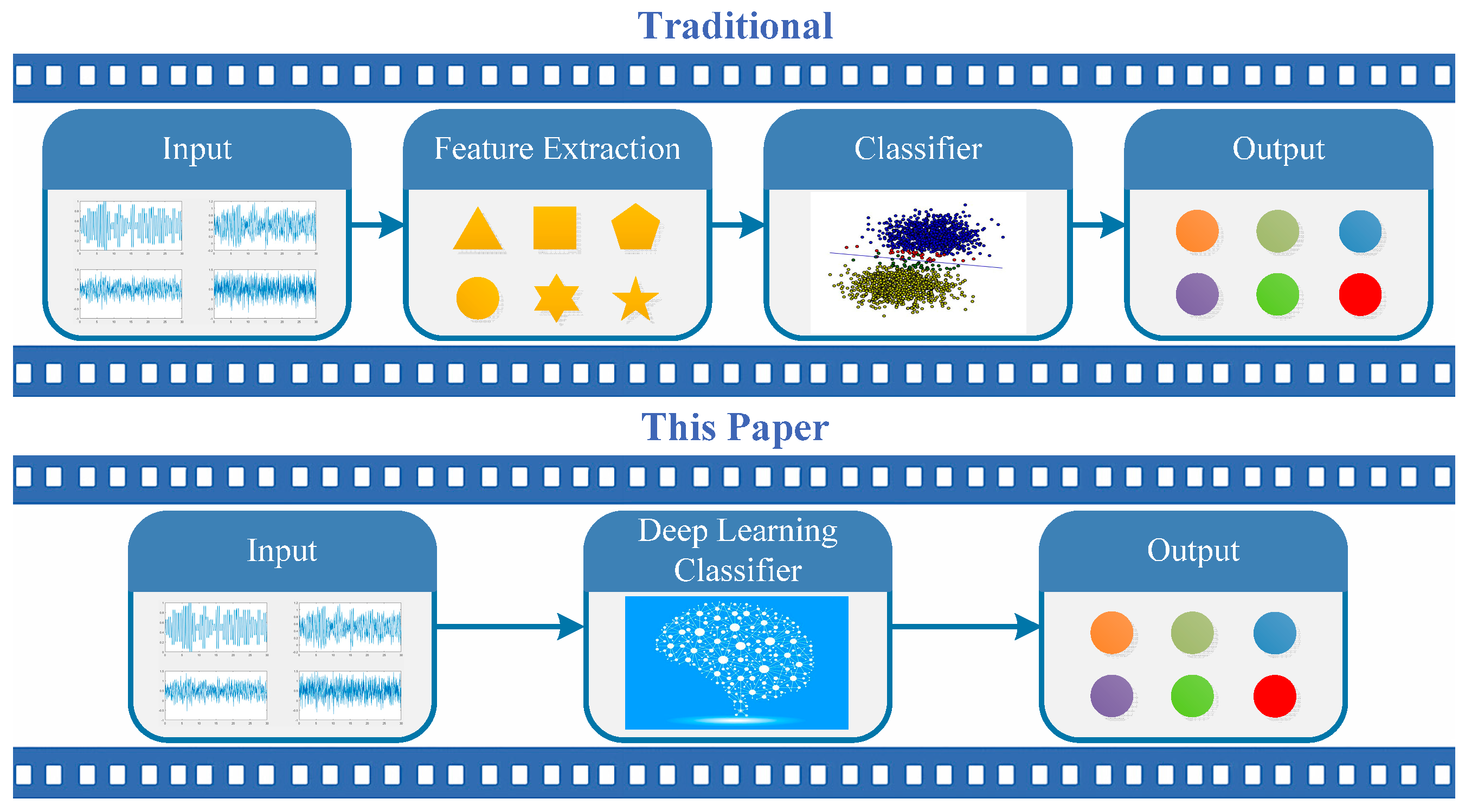
2.1. Conventional Works Based on Separated Features and Classifiers
2.2. CNN-Based Methods
2.3. LSTM-Based Methods
3. Heterogeneous Deep Model Fusion
3.1. Communication Signal Description
3.1.1. Modulation Signal Description
3.1.2. Radio Channel Description
3.2. CNNs
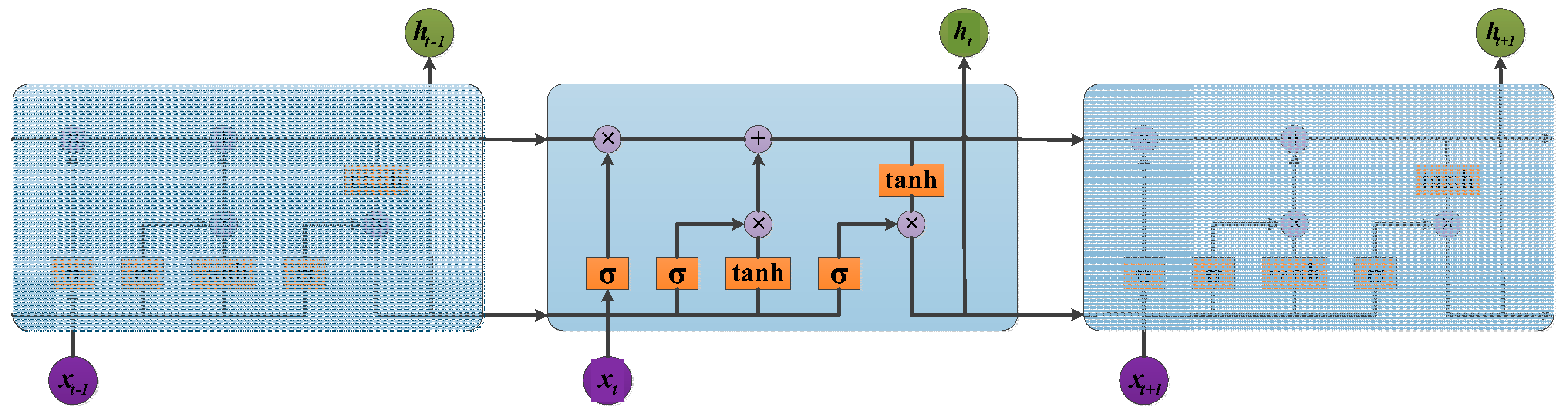
3.3. LSTM
3.4. Fusion Model Based on CNN and LSTM
| Algorithm 1. Training HDMF (parallel) |
| 1: Initialize the parameters in CNN, in LSTM, , in the loss layer, the learning rate , and the number of iterations . |
| 2: While the loss does not converge, do |
| 3: |
| 4: Compute the total loss by . |
| 5: Compute the backpropagation error for each by . |
| 6: Update parameter by |
| 7: Update parameters and by . |
| 8: Update parameter by . |
| 9: End while |
3.5. Communication Signal Generation and Backpropagation
| Algorithm 2. Communication signal generation |
| 1: Open the real geographic environment through the control in Visual Studio. |
| 2: Real-time track transmission and simulation of unmanned aerial vehicle (UAV) flight. |
| 3: Add the latitude and longitude coordinates of the radiation and the height of the antenna. |
| 4: Build an LR channel model based on the parameters of coordinate, climate, and terrain, etc. |
| 5: Generation of baseband signals randomly and in order to generate various modulation signals by MATLAB. |
| 6: The communication between Visual Studio and MATLAB is by means of a User Datagram Protocol (UDP), and the real sample data is generated and finally stored. |
4. Results
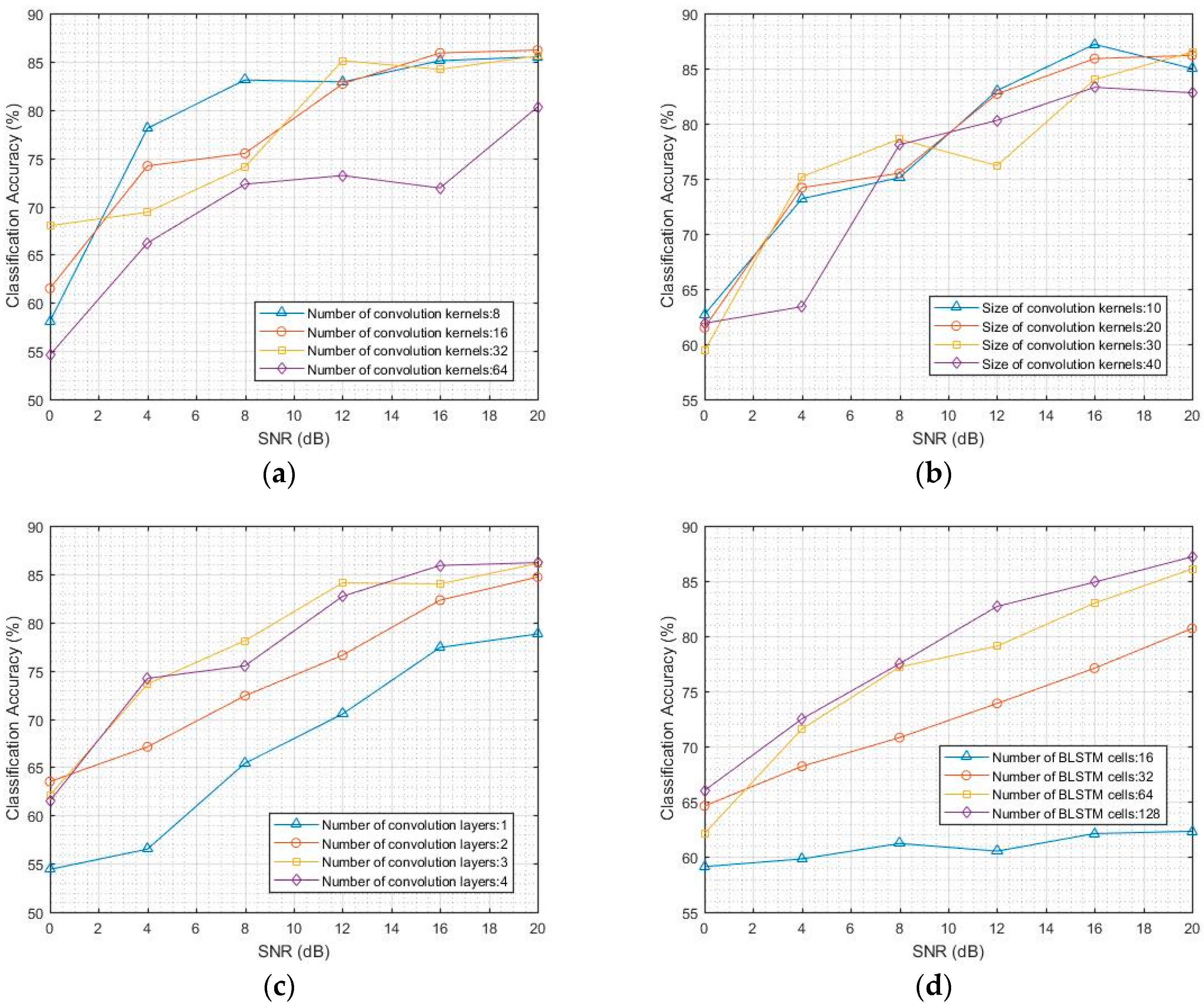
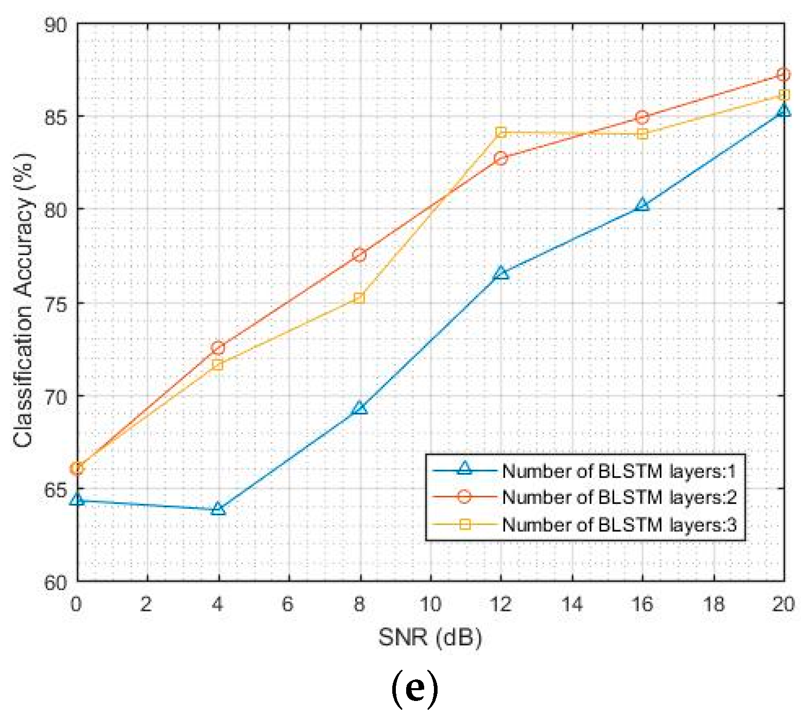
4.1. Classification Accuracy of CNN and LSTM Models
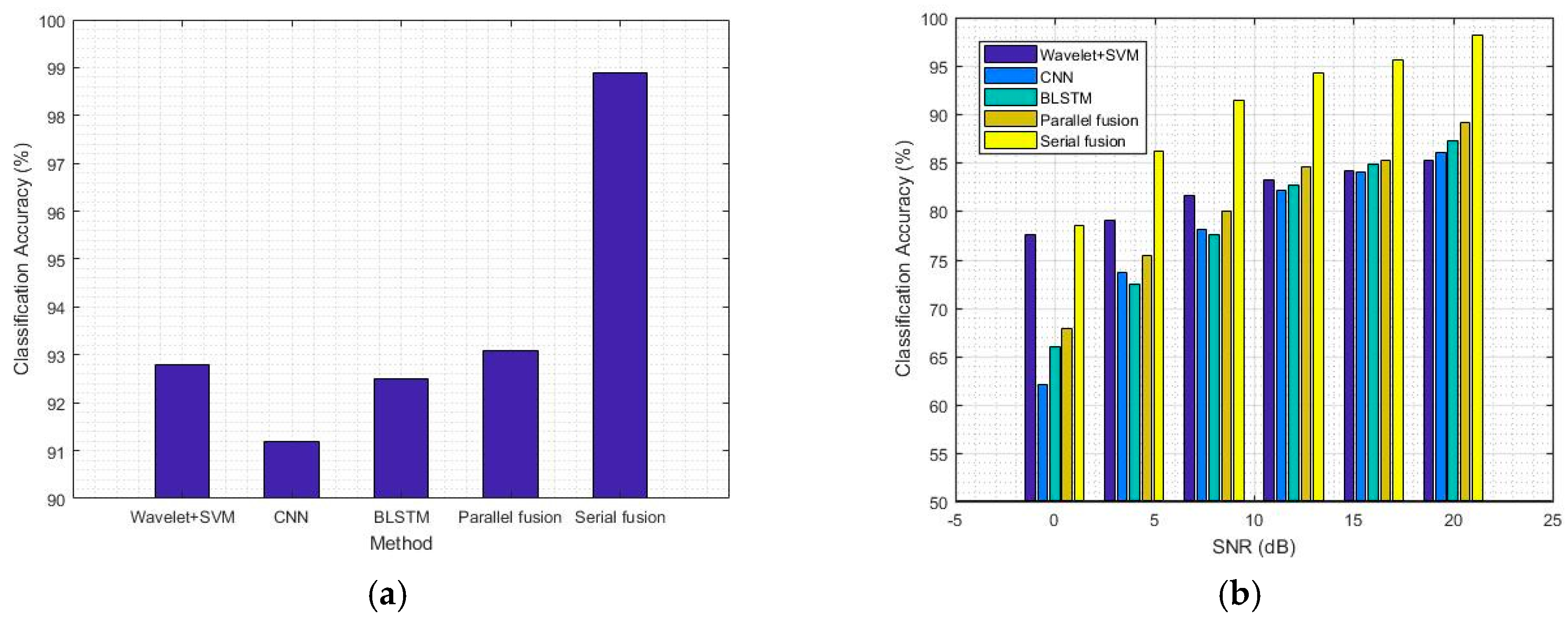
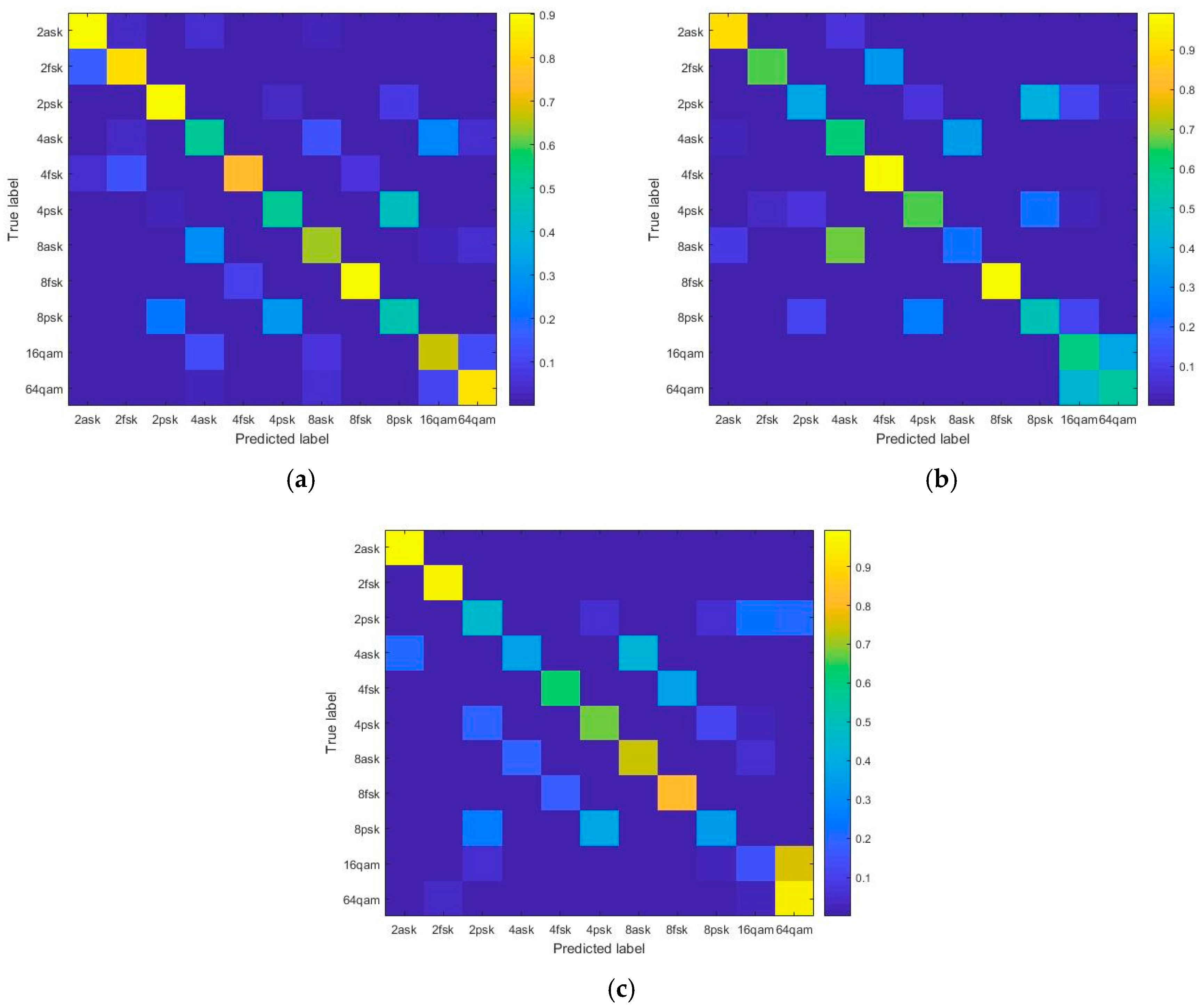
4.2. Comparison of Classification Accuracy between the Deep Learning Models and the Traditional Method
5. Conclusions
Acknowledgments
Author Contributions
Conflicts of Interest
References
- Zheleva, M.; Chandra, R.; Chowdhery, A.; Kapoor, A.; Garnett, P. TX miner: Identifying transmitters in real-world spectrum measurements. In Proceedings of the IEEE International Symposium on Dynamic Spectrum Access Networks (DySPAN), Stockholm, Sweden, 29 September–2 October 2015; pp. 94–105. [Google Scholar]
- Hong, S.S.; Katti, S.R. Dof: A local wireless information plane. In Proceedings of the ACM SIGCOMM 2011 Conference, Toronto, ON, Canada, 15–19 August 2011; ACM: New York, NY, USA, 2011; pp. 230–241. [Google Scholar]
- Dobre, O.A.; Abdi, A.; Bar-Ness, Y.; Su, W. Survey of automatic modulation classification techniques: Classical approaches and new trends. IET Commun. 2007, 1, 137–156. [Google Scholar] [CrossRef]
- Gardner, W.A. Signal interception: A unifying theoretical framework for feature detection. IEEE Trans. Commun. 1988, 36, 897–906. [Google Scholar] [CrossRef]
- Yu, Z. Automatic Modulation Classification of Communication Signals. Ph.D. Thesis, Department of Electrical and Computer Engineering, New Jersey Institute of Technology, Newark, NI, USA, 2006. [Google Scholar]
- Dandawate, A.V.; Giannakis, G.B. Statistical tests for presence of cyclostationarity. IEEE Trans. Signal Process. 1994, 42, 2355–2369. [Google Scholar] [CrossRef]
- Fehske, A.; Gaeddert, J.; Reed, J.H. A new approach to signal classification using spectral correlation and neural networks. In Proceedings of the First IEEE International Symposium on New Frontiers in Dynamic Spectrum Access Networks, Baltimore, MD, USA, 8–11 November 2005; pp. 144–150. [Google Scholar]
- LeCun, Y.; Bengio, Y.; Hinton, G. Deep learning. Nature 2015, 521, 436–444. [Google Scholar] [CrossRef] [PubMed]
- O’Shea, T.J.; Corgan, J.; Clancy, T.C. Convolutional radio modulation recognition networks. In Proceedings of the International Conference on Engineering Applications of Neural Networks, Aberdeen, UK, 2–5 September 2016; pp. 213–226. [Google Scholar]
- Hochreiter, S.; Schmidhuber, J. Long short-term memory. Neural Comput. 1997, 9, 1735–1780. [Google Scholar] [CrossRef] [PubMed]
- Lopatka, J.; Pedzisz, M. Automatic modulation classification using statistical moments and a fuzzy classifier. In Proceedings of the 5th International Conference on Signal Processing Proceedings, Beijing, China, 21–25 August 2000; pp. 1500–1506. [Google Scholar]
- Yang, Y.; Soliman, S. Optimum classifier for M-ary PSK signals. In Proceedings of the ICC 91 International Conference on Communications Conference Record, Denver, CO, USA, 23–26 June 1991; pp. 1693–1697. [Google Scholar]
- Shermeh, A.E.; Ghazalian, R. Recognition of communication signal types using genetic algorithm and support vector machines based on the higher order statistics. Digit. Signal Process. 2010, 20, 1748–1757. [Google Scholar] [CrossRef]
- Sherme, A.E. A novel method for automatic modulation recognition. Appl. Soft Comput. 2012, 12, 453–461. [Google Scholar] [CrossRef]
- Panagiotou, P.; Anastasopoulos, A.; Polydoros, A. Likelihood ratio tests for modulation classification. In Proceedings of the 21st Century Military Communications Conference Proceedings, Los Angeles, CA, USA, 22–25 October 2000; pp. 670–674. [Google Scholar]
- Wong, M.; Nandi, A. Automatic digital modulation recognition using spectral and statistical features with multi-layer perceptions. In Proceedings of the Sixth International Symposium on Signal Processing and its Applications, Kuala Lumpur, Malaysia, 13–16 August 2001; pp. 390–393. [Google Scholar]
- Basheer, I.A.; Hajmeer, M. Artificial neural networks: Fundamentals, computing, design, and application. J. Microbiol. Methods 2000, 43, 3–31. [Google Scholar] [CrossRef]
- Iliadis, L.S.; Maris, F. An artificial neural network model for mountainous water-resources management: The case of Cyprus mountainous watersheds. Environ. Model. Softw. 2007, 22, 1066–1072. [Google Scholar] [CrossRef]
- Ali, A.; Yangyu, F. Unsupervised feature learning and automatic modulation classification using deep learning model. Phys. Commun. 2017, 25, 75–84. [Google Scholar] [CrossRef]
- Ali, A.; Yangyu, F.; Liu, S. Automatic modulation classification of digital modulation signals with stacked autoencoders. Digit. Signal Process. 2017, 71, 108–116. [Google Scholar] [CrossRef]
- Ji, S.; Xu, W.; Yang, M.; Yu, K. 3D convolutional neural networks for human action recognition. IEEE Trans. Pattern Anal. Mach. Intell. 2013, 35, 221–231. [Google Scholar] [CrossRef] [PubMed]
- Karpathy, A.; Toderici, G.; Shetty, S.; Leung, T.; Sukthankar, R.; Li, F. Large-scale video classification with convolutional neural networks. In Proceedings of the 2014 IEEE Conference on Computer Vision and Pattern Recognition, Columbus, OH, USA, 23–28 June 2014. [Google Scholar]
- Luan, S.; Zhang, B.; Chen, C.; Han, J.; Liu, J. Gabor Convolutional Networks. arXiv, 2017; arXiv:1705.01450. [Google Scholar]
- Zhang, B.; Gu, J.; Chen, C.; Han, J.; Su, X.; Cao, X.; Liu, J. One-Two-One network for Compression Artifacts Reduction in Remote Sensing. ISPRS J. Photogramm. Remote Sens. 2018. [Google Scholar] [CrossRef]
- Duong, T.; Bui, H.; Phung, D.; Venkatesh, S. Activity recognition and abnormality detection with the switching hidden semi-markov model. In Proceedings of the 2005 IEEE Computer Society Conference on Computer Vision and Pattern Recognition, San Diego, CA, USA, 20–25 June 2005. [Google Scholar]
- Sminchisescu, C.; Kanaujia, A.; Li, Z.; Metaxas, D. Conditional models for contextual human motion recognition. In Proceedings of the Tenth IEEE International Conference on Computer Vision, Beijing, China, 17–21 October 2005. [Google Scholar]
- Ikizler, N.; Forsyth, D. Searching video for complex activities with finite state models. In Proceedings of the 2007 IEEE Conference on Computer Vision and Pattern Recognition, Minneapolis, MN, USA, 17–22 June 2007. [Google Scholar]
- Srivastava, N.; Mansimov, E.; Salakhutdinov, R. Unsupervised learning of video representations using LSTMs. In Proceedings of the 32nd International Conference on International Conference on Machine Learning, Lille, France, 6–11 July 2015. [Google Scholar]
- Donahue, J.; Hendricks, L.A.; Guadarrama, S.; Rohrbach, M.; Venugopalan, S.; Saenko, K.; Darrell, T. Long-term recurrent convolutional networks for visual recognition and description. IEEE Trans. Pattern Anal. Mach. Intell. 2015, 39, 677–691. [Google Scholar] [CrossRef] [PubMed]
- Ng, J.Y.; Hausknecht, M.J.; Vijayanarasimhan, S.; Vinyals, O.; Monga, R.; Toderici, G. Beyond short snippets: Deep networks for video classification. In Proceedings of the 2015 IEEE Conference on Computer Vision and Pattern Recognition, Boston, MA, USA, 7–12 June 2015. [Google Scholar]
- Wu, Z.; Wang, X.; Jiang, Y.; Ye, H.; Xue, X. Modeling spatial-temporal clues in a hybrid deep learning framework for video classification. In Proceedings of the 23rd ACM International Conference on Multimedia, Brisbane, Australia, 26–30 October 2015. [Google Scholar]
- Venugopalan, S.; Rohrbach, M.; Donahue, J.; Mooney, R.J.; Darrell, T.; Saenko, K. Sequence to sequence—Video to text. In Proceedings of the 2015 IEEE International Conference on Computer Vision, Los Alamitos, CA, USA, 7–13 December 2015. [Google Scholar]
- Lazebnik, S.; Schmid, C.; Ponce, J. Beyond bags of features: Spatial pyramid matching for recognizing natural scene categories. In Proceedings of the 2006 IEEE Computer Society Conference on Computer Vision and Pattern Recognition, New York, NY, USA, 17–22 June 2006. [Google Scholar]
- Zhang, B.; Yang, Y.; Chen, C.; Han, J.; Shao, L. Action Recognition Using 3D Histograms of Texture and A Multi-class Boosting Classifier. IEEE Trans. Image Process. 2017, 26, 4648–4660. [Google Scholar] [CrossRef] [PubMed]
- Li, C.; Xie, C.; Zhang, B.; Chen, C.; Han, J. Deep Fisher Discriminant Learning for Mobile Hand Gesture Recognition. Pattern Recognit. 2018, 77, 276–288. [Google Scholar] [CrossRef]
- Yao, L.; Torabi, A.; Cho, K.; Ballas, N.; Pal, C.; Larochelle, H.; Courville, A. Describing videos by exploiting temporal structure. In Proceedings of the 2015 IEEE International Conference on Computer Vision, Santiago, Chile, 7–13 December 2015. [Google Scholar]
- Zhang, B.; Luan, S.; Chen, C.; Han, J.; Shao, L. Latent Constrained Correlation Filter. IEEE Trans. Image Process. 2017, 27, 1038–1048. [Google Scholar] [CrossRef]
- Abadi, M.; Agarwal, A.; Barham, P.; Brevdo, E.; Chen, Z.; Citro, C.; Corrado, G.S.; Davis, A.; Dean, J.; Devin, M.; et al. Tensorflow: Large-scale machine learning on heterogeneous distributed systems. In Proceedings of the 12th USENIX Conference on Operating Systems Design and Implementation, Savannah, GA, USA, 2–4 November 2016. [Google Scholar]
- Kingma, D.P.; Ba, J. Adam: A Method for Stochastic Optimization. CORR. Available online: http://arxiv.org/abs/1412.6980 (accessed on 1 March 2018).
- Voulodimos, A.; Doulamis, N.; Doulamis, A.; Protopapadakis, E. Deep learning for computer vision: A brief review. Comput. Intell. Neurosci. 2018, 2018, 7068349. [Google Scholar] [CrossRef] [PubMed]
- Wang, Z.; Hu, R.; Chen, C.; Yu, Y.; Jiang, J.; Liang, C.; Satoh, S. Person Re-identification via Discrepancy Matrix and Matrix Metric. IEEE Trans. Cybern. 2017, 1–5. [Google Scholar] [CrossRef]
- Ding, M.; Fan, G. Articulated and Generalized Gaussian Kernel Correlation for Human Pose Estimation. IEEE Trans. Image Process. 2016, 25, 776–789. [Google Scholar] [CrossRef] [PubMed]


| Content | Detailed description |
|---|---|
| Modulation mode | Eleven types of single-carrier modulation modes (MASK, MFSK, MPSK, MQAM) |
| Carrier frequency | 20 MHz to 2 GHz |
| Noise | 0 dB to 20 dB |
| Attenuation | A fading channel based on a real geographical environment |
| Sample value | 22,000 samples (11,000 training samples and 11,000 test samples) |
| Kernels | Parameters (M) | Training Time (s) | Testing Time (s) | |
|---|---|---|---|---|
| CNN1 (with size 20) | 8 | 1.537 | 72 | 0.4 |
| 16 | 3.073 | 96 | 0.6 | |
| 32 | 6.146 | 118 | 1.1 | |
| CNN2 (with size 20) | 8-8 | 1.539 | 96 | 1.0 |
| 16-16 | 3.079 | 144 | 1.5 | |
| 32-32 | 6.166 | 250.5 | 2.85 | |
| CNN3 (with size 20) | 8-8-8 | 1.540 | 148 | 1.55 |
| 16-16-16 | 3.084 | 196 | 2.16 | |
| 32-32-32 | 6.187 | 420 | 4.3 | |
| CNN4 (with size 20) | 8-8-8-8 | 1.541 | 165 | 2.3 |
| 16-16-16-16 | 3.089 | 296.5 | 3.3 | |
| 32-32-32-32 | 6.207 | 507.5 | 5.9 |
| Methods | Wavelet/SVM | CNN | Bi-LSTM | Parallel Fusion | Serial Fusion |
|---|---|---|---|---|---|
| Accuracy | 92.8% | 91.2% | 92.5% | 93.1% | 98.9% |
| SNR Methods | 20 dB | 16 dB | 12 dB | 8 dB | 4 dB | 0 dB |
|---|---|---|---|---|---|---|
| Wavelet/SVM | 85.2% | 84.1% | 83.2% | 81.6% | 79.0% | 77.5% |
| CNN | 86.1% | 84.0% | 82.1% | 78.1% | 73.6% | 62.1% |
| Bi-LSTM | 87.2% | 84.9% | 82.7% | 77.5% | 72.5% | 66.0% |
| Parallel fusion | 89.1% | 85.2% | 84.6% | 80.0% | 75.4% | 67.9% |
| Serial fusion | 98.2% | 95.6% | 94.3% | 91.5% | 86.2% | 78.5% |
© 2018 by the authors. Licensee MDPI, Basel, Switzerland. This article is an open access article distributed under the terms and conditions of the Creative Commons Attribution (CC BY) license (http://creativecommons.org/licenses/by/4.0/).
Share and Cite
Zhang, D.; Ding, W.; Zhang, B.; Xie, C.; Li, H.; Liu, C.; Han, J. Automatic Modulation Classification Based on Deep Learning for Unmanned Aerial Vehicles. Sensors 2018, 18, 924. https://doi.org/10.3390/s18030924
Zhang D, Ding W, Zhang B, Xie C, Li H, Liu C, Han J. Automatic Modulation Classification Based on Deep Learning for Unmanned Aerial Vehicles. Sensors. 2018; 18(3):924. https://doi.org/10.3390/s18030924
Chicago/Turabian StyleZhang, Duona, Wenrui Ding, Baochang Zhang, Chunyu Xie, Hongguang Li, Chunhui Liu, and Jungong Han. 2018. "Automatic Modulation Classification Based on Deep Learning for Unmanned Aerial Vehicles" Sensors 18, no. 3: 924. https://doi.org/10.3390/s18030924
APA StyleZhang, D., Ding, W., Zhang, B., Xie, C., Li, H., Liu, C., & Han, J. (2018). Automatic Modulation Classification Based on Deep Learning for Unmanned Aerial Vehicles. Sensors, 18(3), 924. https://doi.org/10.3390/s18030924