Research on Flow Field Perception Based on Artificial Lateral Line Sensor System

 , , and
Abstract
:1. Introduction
2. Biomechanical Model of Lateral Line
- Flow velocity estimation
- Attitude perception
- Obstacle identification.
3. Optimal Topology of Sensors
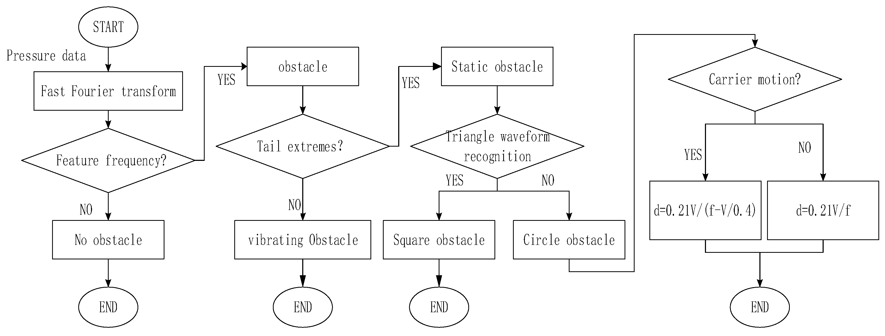
4. Obstacle Sensing Algorithm Based on Simulation
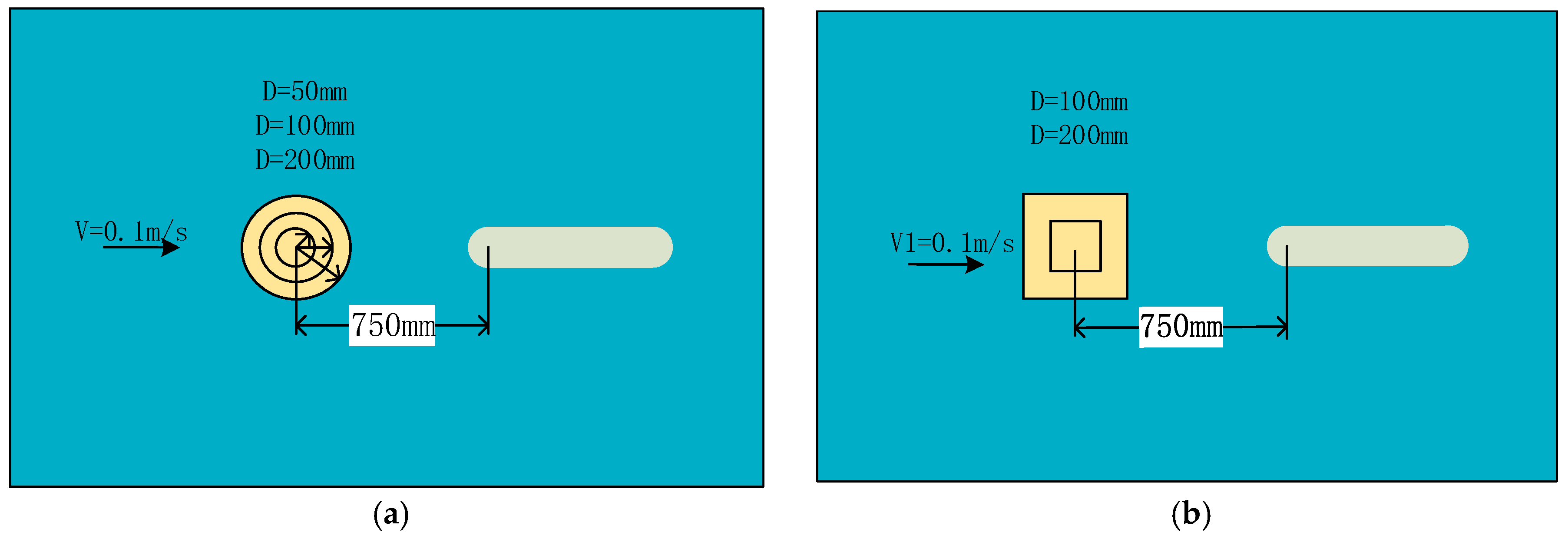
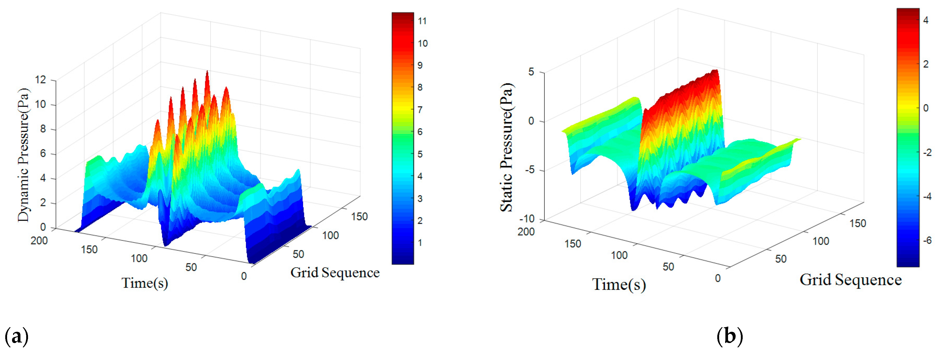
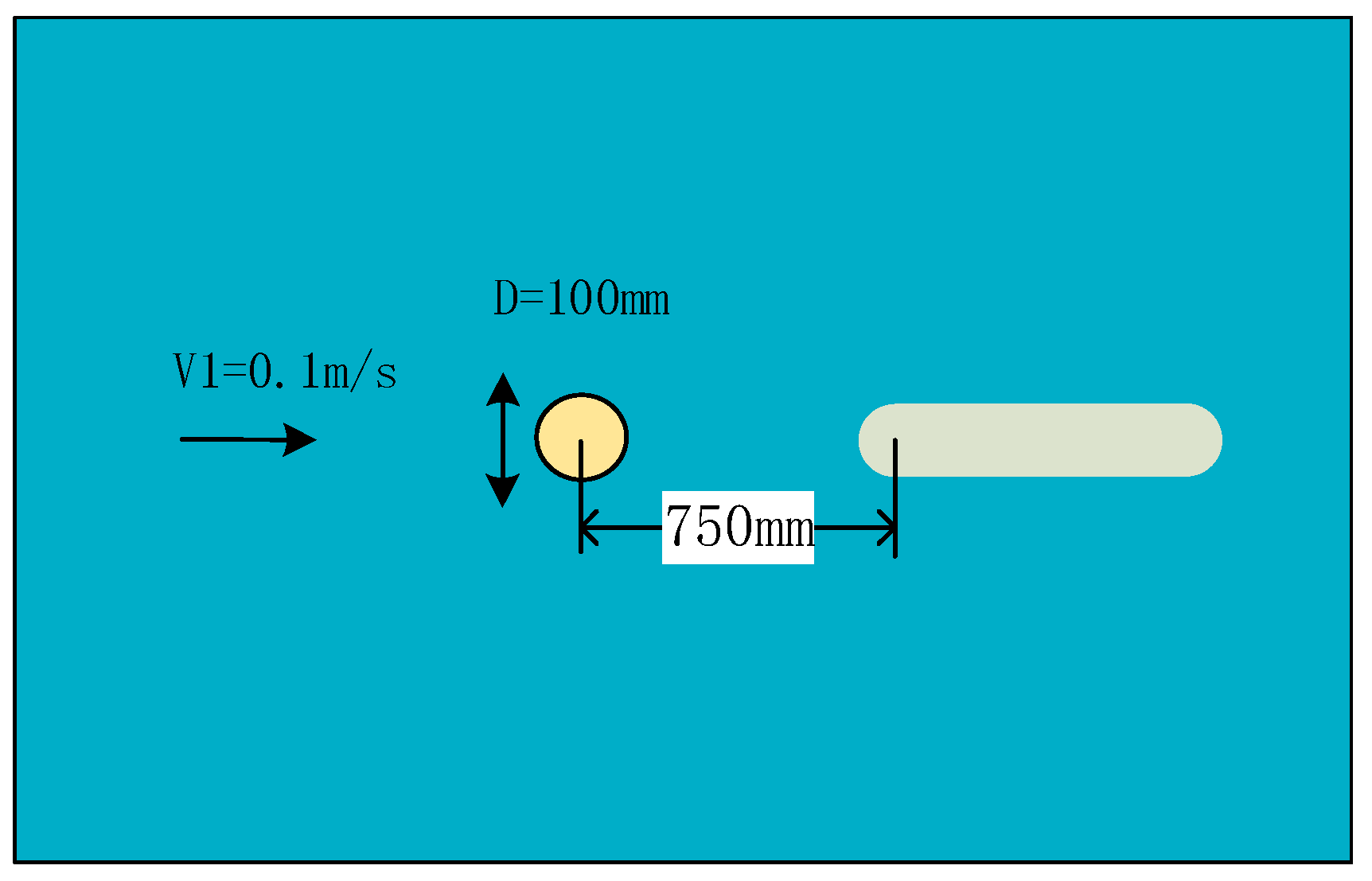
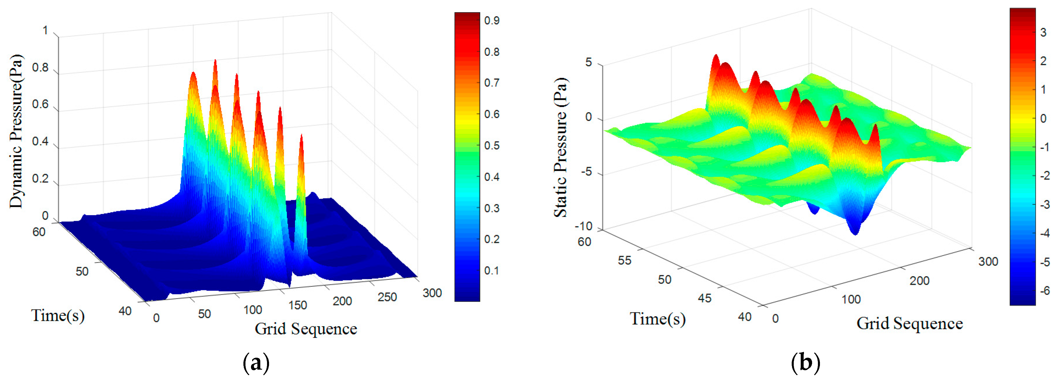
4.1. Simulation of Static Obstacle
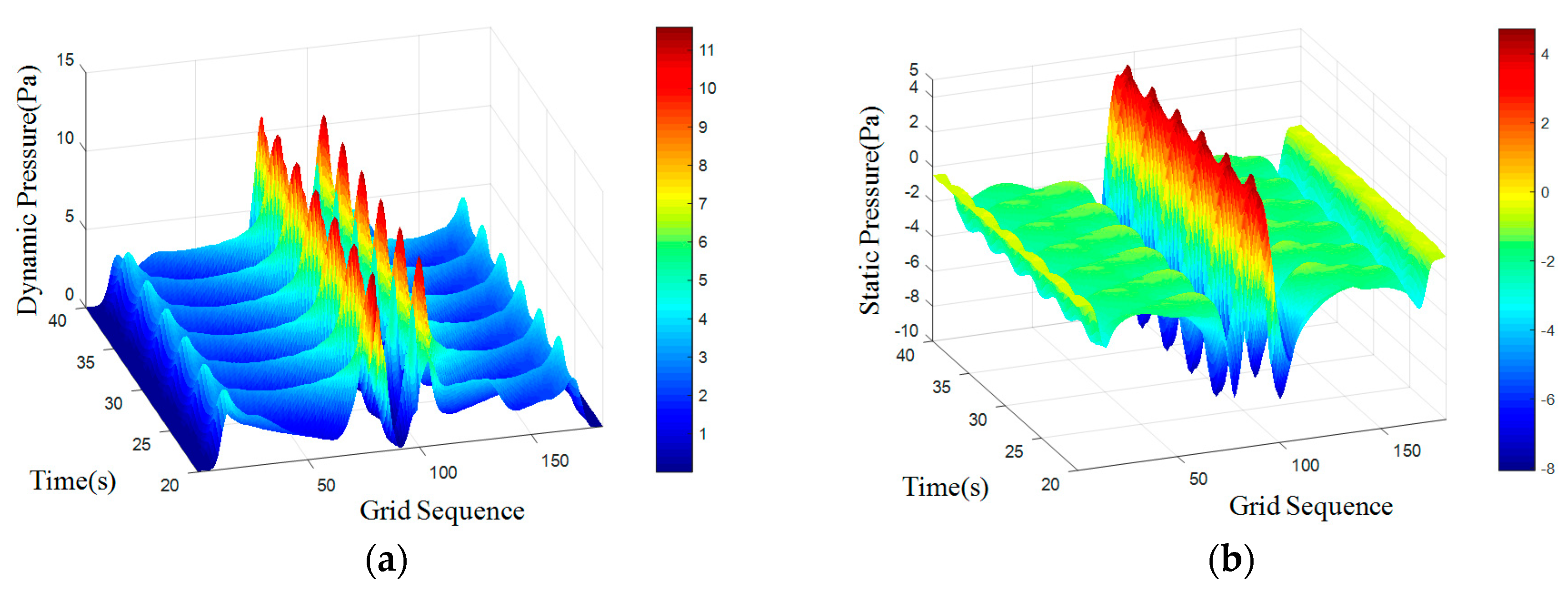
4.2. Simulation of Moving Carrier
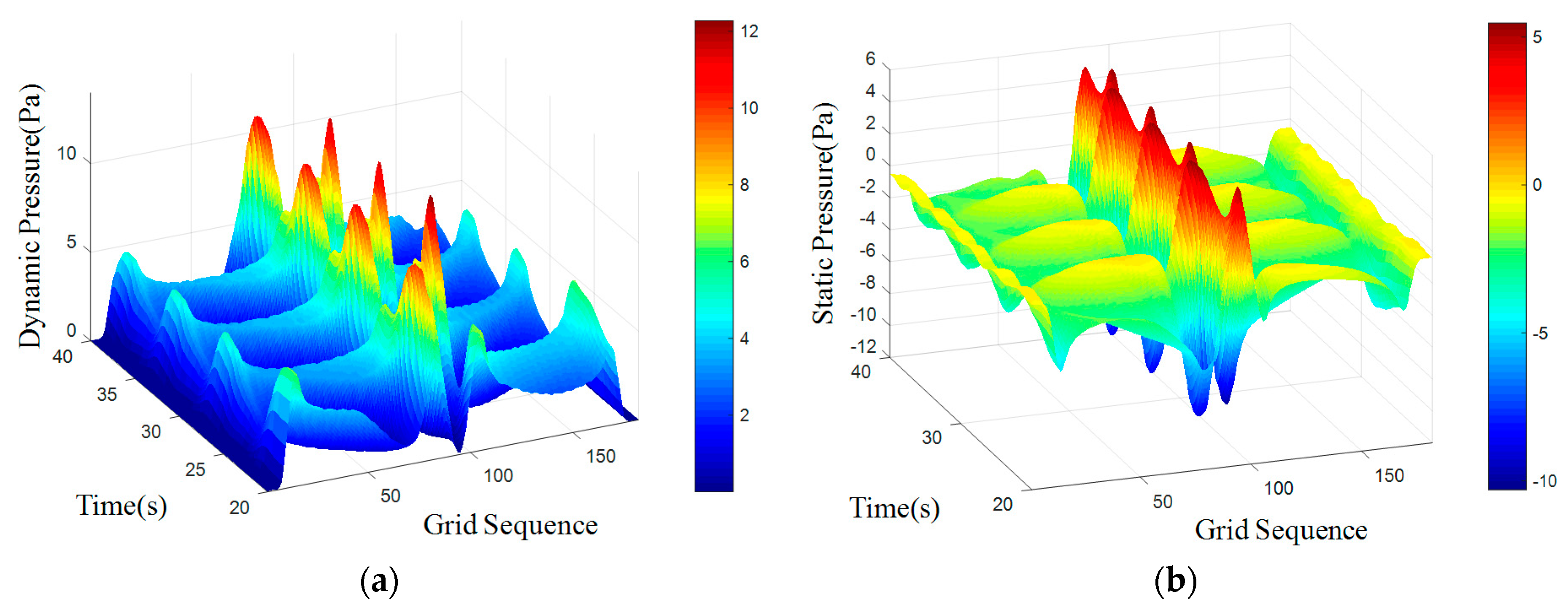
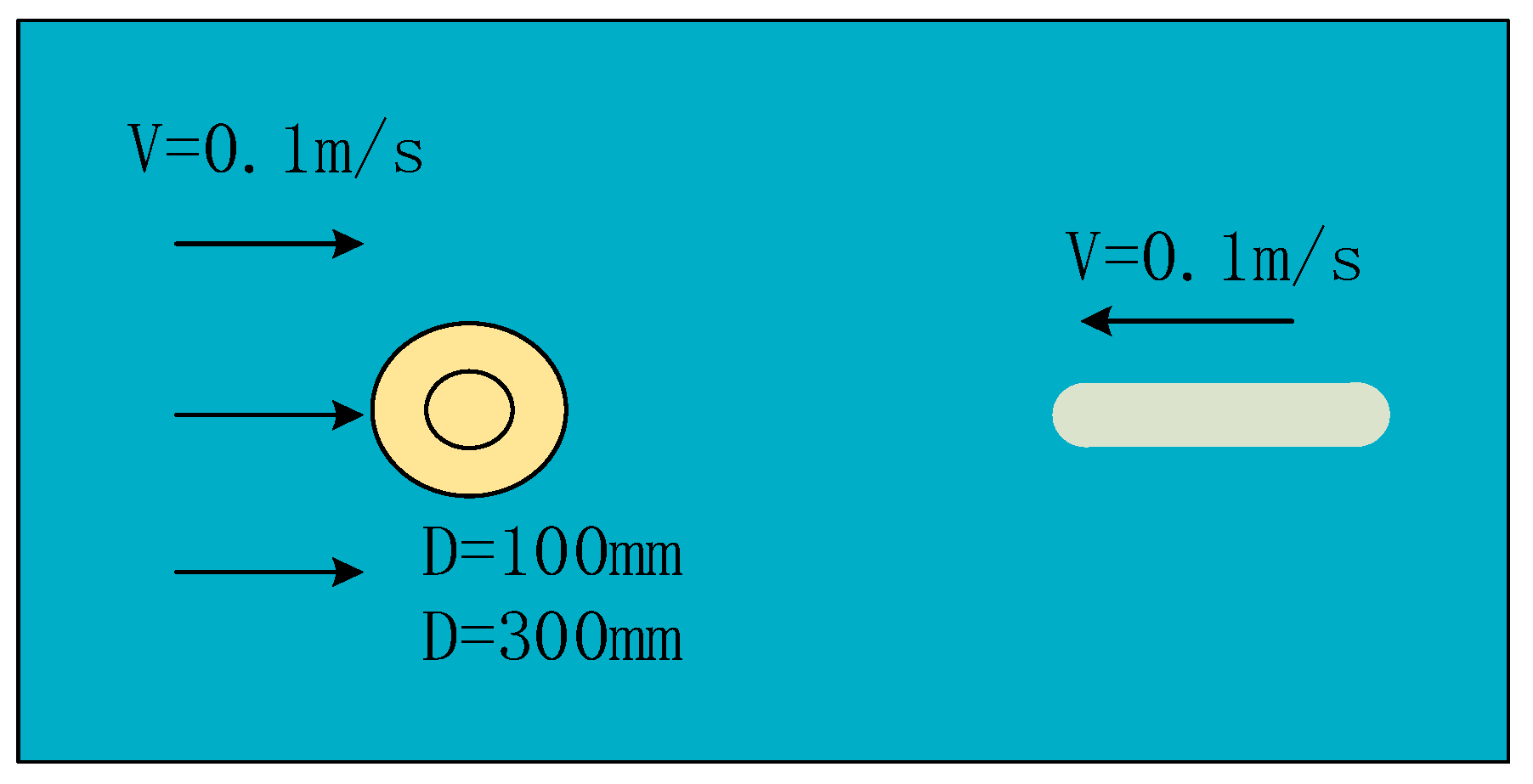
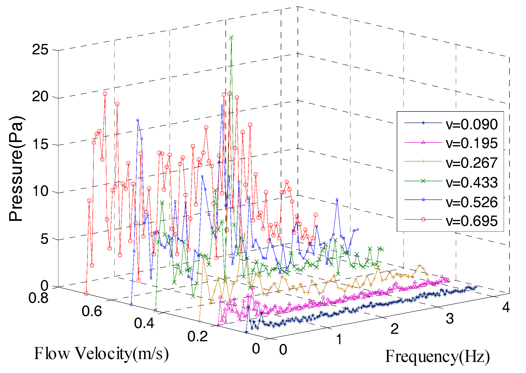
4.3. Simulation of Vibrating Obstacle
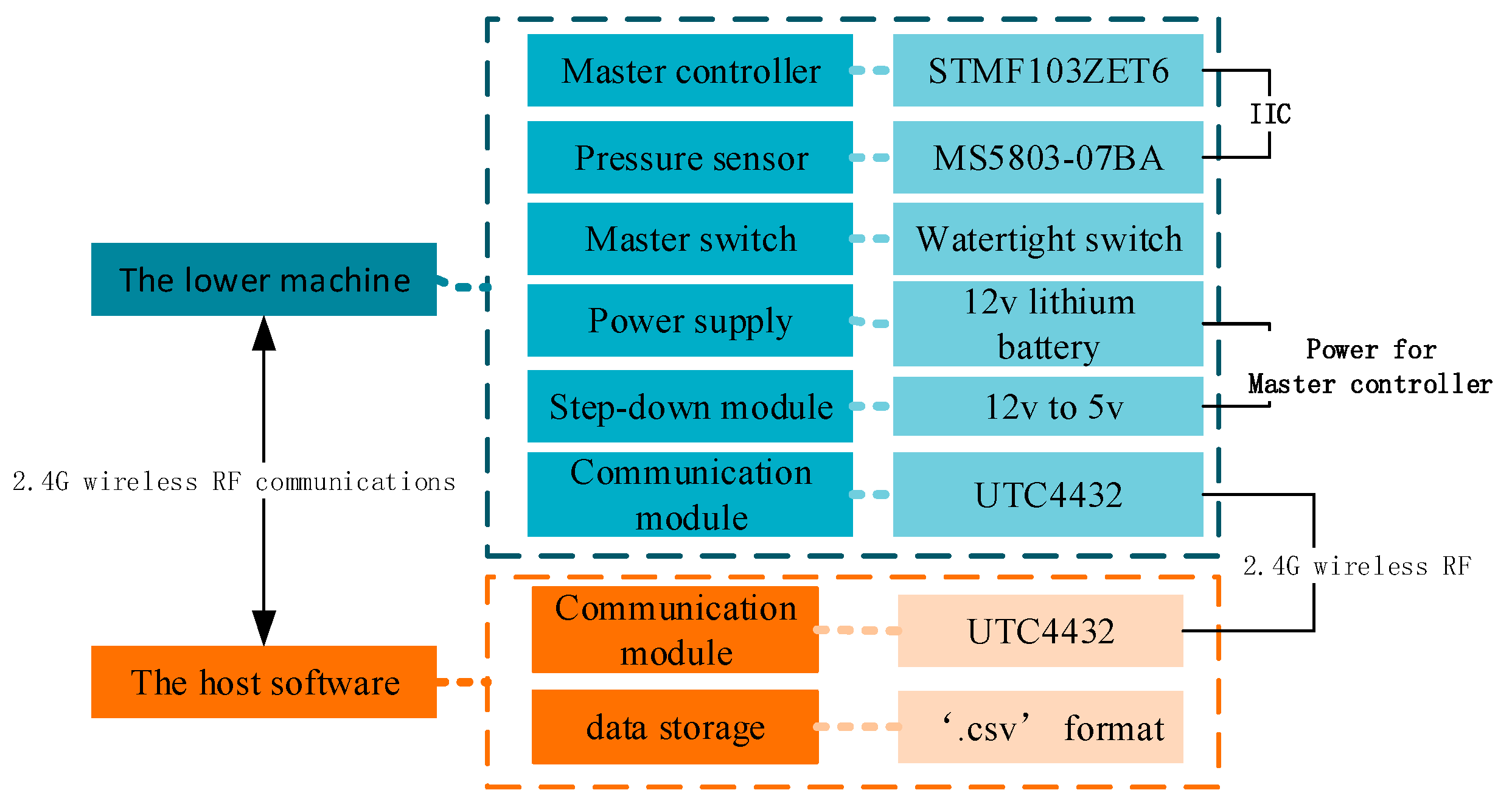
5. Experiments of Artificial Lateral Line
5.1. Experiments Design
5.2. Underwater Experiments
6. Experimental Analysis of Artificial Lateral Line
6.1. Hydrostatic Correction
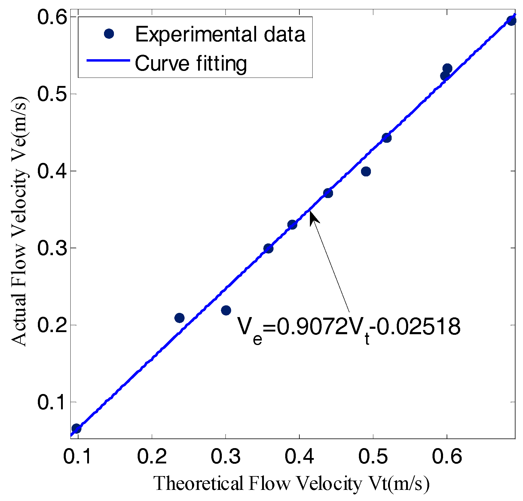
6.2. Velocity Estimation
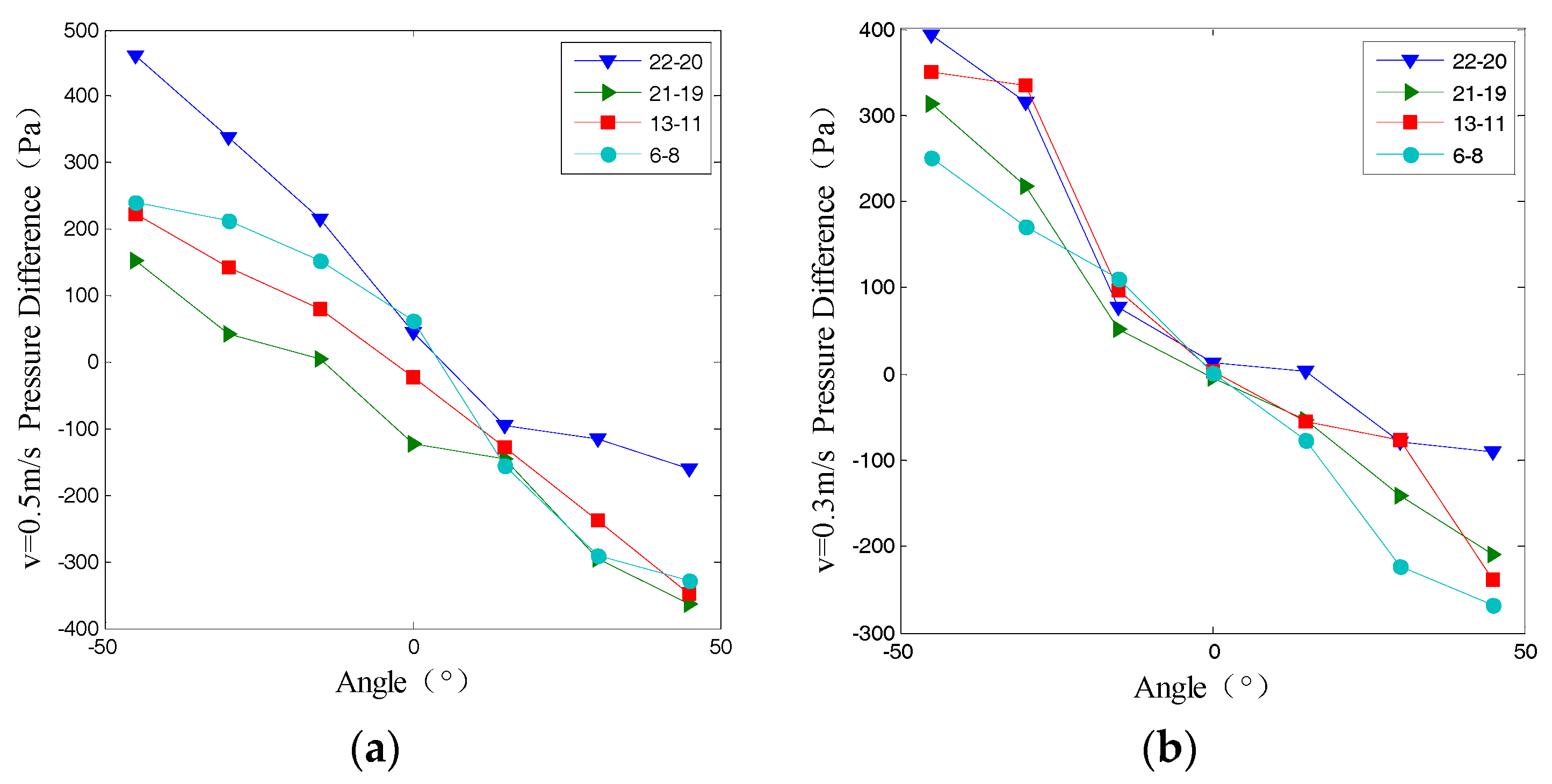
6.3. Attitude Perception
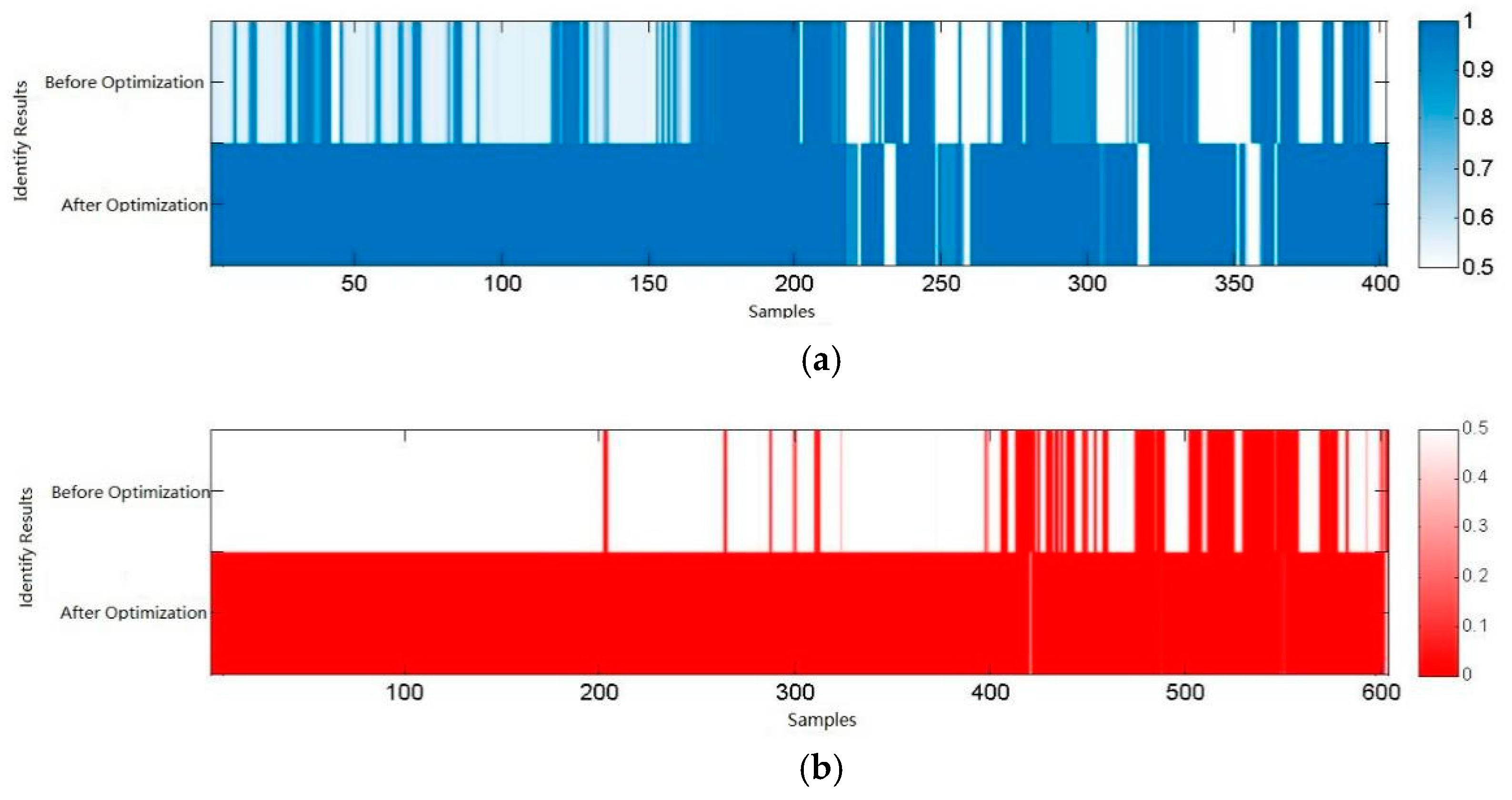
6.4. Obstacle Identification
7. Conclusions
Acknowledgments
Author Contributions
Conflicts of Interest
References
- Krahe, R.; Maler, L. Neural maps in the electrosensory system of weakly electric fish. Curr. Opin. Neurobiol. 2014, 24, 13–21. [Google Scholar] [CrossRef] [PubMed]
- Blaxter, J.H.S.; Fuiman, L.A. The Mechanosensory Lateral Line: Neurobiology and Evolution; Coombs, S., Gorner, P., Munz, H., Eds.; Springer Science & Business Media: Berlin, German, 2012; pp. 481–499. [Google Scholar]
- Kanter, M.J.; Coombs, S. Rheotaxis and prey detection in uniform currents by Lake Michigan mottled sculpin. J. Exp. Biol. 2003, 206, 59–70. [Google Scholar] [CrossRef] [PubMed]
- Gibbs, M.A. Lateral line receptors: Where do they come from developmentally and where is our research going. Brain Behav. Evol. 2004, 64, 163–181. [Google Scholar] [CrossRef] [PubMed]
- Hoekstra, D.; Janssen, J. Non-visual feeding behavior of the mottled sculpin, Cottus bairdi, in Lake Michigan Environ. Biol. Fishes 2006, 12, 111–117. [Google Scholar] [CrossRef]
- Yang, Y.; Nguyen, N.; Chen, N.; Lockwood, M.; Tucker, C.; Hu, H.; Bleckmann, H.; Liu, C.; Jones, D.L. Artificial lateral line with biomimetic neuromasts to emulate fish sensing. Bioinspir. Biomim. 2010, 5, 16001. [Google Scholar] [CrossRef] [PubMed]
- Fan, Z.; Chen, J.; Zou, J.; Bullen, D.; Liu, C.; Delcomyn, F. Design and fabrication of artificial lateral line flow sensors. J. Micromech. Microeng. 2002, 12, 655–661. [Google Scholar] [CrossRef]
- Kroese, A.B.A.; Schellart, N.A.M. Velocity- and acceleration-sensitive units in the trunk lateral line of the trout. J. Neurophys. 1992, 68, 2212–2221. [Google Scholar] [CrossRef] [PubMed]
- Pohlmann, K.; Atema, J.; Breithaupt, T. The importance of the lateral line in nocturnal predation of piscivorous catfish. J. Exper. Biol. 2004, 207, 2971–2978. [Google Scholar] [CrossRef] [PubMed]
- Bleckmann, H. 3-D ofientation with the octavolateralis system. J. Physiol. Paris 2004, 98, 53–65. [Google Scholar] [CrossRef] [PubMed]
- Pandya, S.; Yang, Y.; Liu, C. Biomimetic Imaging of Flow Phenomena. Int. Conf. Acoust. Speech Signal Process. 2007, 2, II-933–II-936. [Google Scholar]
- DeVries, L.; Lagor, F.D.; Lei, H.; Tan, X.; Paley, D.A. Distributed flow estimation and closed-loop control of an underwater vehicle with a multi-modal artificial lateral line. Bioinspir. Biomim. 2015, 10, 025002. [Google Scholar] [CrossRef] [PubMed]
- Netten, S.M.V. Hydrodynamics of the excitation of the cupula in the fish canal lateral line. Vet. Dermatol. 1991, 18, 324–331. [Google Scholar] [CrossRef]
- Chambers, L.D.; Akanyeti, O.; Venturelli, R. A fish perspective: Detecting flow features while moving using an artificial lateral line in steady and unsteady flow. J. R. Soc. Interface 2014, 11. [Google Scholar] [CrossRef] [PubMed]
- Netten, S.M.V. Hydrodynamics detection by cupulae in a lateral-line canal: Functional relations between physics and physiology. Biol. Cybern. 2006, 94, 67–85. [Google Scholar] [CrossRef] [PubMed]
- Venturelli, R.; Akanyeti, O.; Visentin, F.; Ježov, J.; Chambers, L.D.; Toming, G.; Brow, J.; Kruusmaa, M.; Megill, W.M.; Fiorini, P. Hydrodynamic pressure sensing with an artificial lateral line in steady and unsteady flows. Bioinspir. Biomim. 2012, 7, 36004–36015. [Google Scholar] [CrossRef] [PubMed]
- Tan, S. Underwater artificial lateral line flow sensors. Microsyst. Technol. 2014, 20, 2123–2136. [Google Scholar]
- Wannenburg, J.; Malekian, R. Physical Activity Recognition from Smartphone Accelerometer Data for User Context Awareness Sensing. IEEE Trans. Syst. Man Cybern. Syst. 2017, 47, 3142–3149. [Google Scholar] [CrossRef]
- Tian, Z.; Liu, F.; Li, Z.; Malekian, R.; Xie, Y. The Development of Key Technologies in Applications of Vessels Connected to the Internet. Symmetry 2017, 9, 211. [Google Scholar] [CrossRef]
- Yu, J.; Malekian, R.; Chang, J.; Su, B. Modeling of whole-space transient electromagnetic responses based on FDTD and its application in the mining industry. IEEE Trans. Ind. Inform. 2017, 13, 2974–2982. [Google Scholar] [CrossRef]


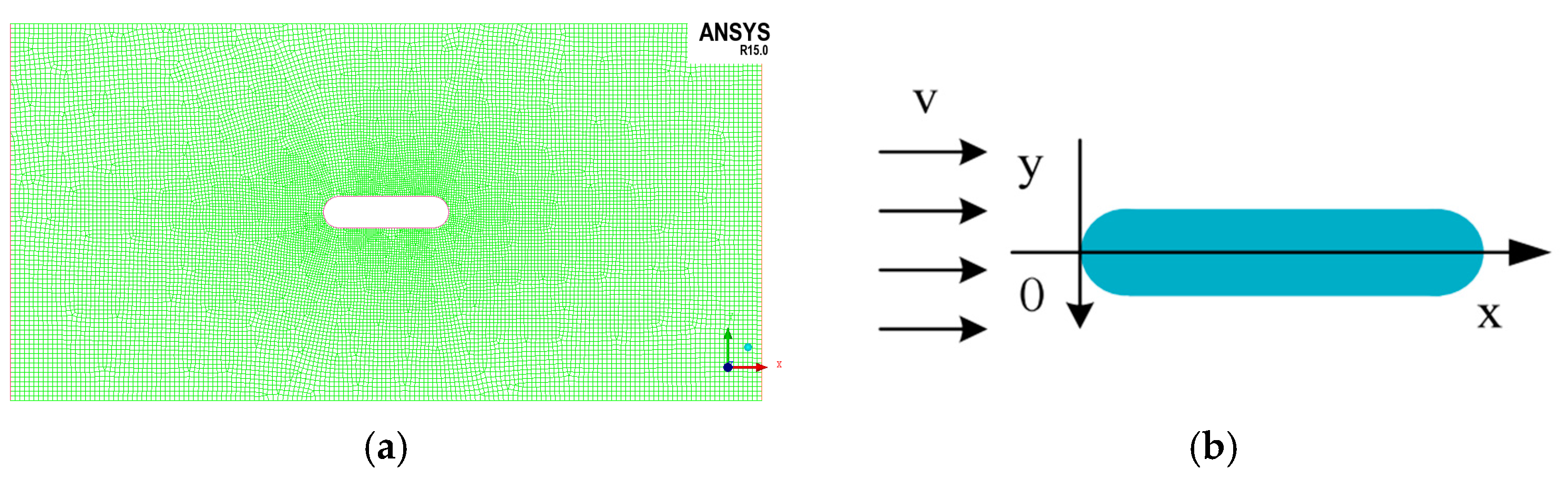
| Mesh (Icem) | |||
| Fluid Dimensions | 1 m × 3 m | Carrier Dimensions | 0.1 m × 0.4 m |
| Number of Grids | 232,776 | Grid type | Unstructured grids |
| Hydrodynamic Simulation (Fluent) | |||
| Physical model | Standard K- model | Boundary conditions | Velocity inlet/pressure outlet |
| Inlet velocity | −1 m/s | Reynolds number | 49,900–499,000 |
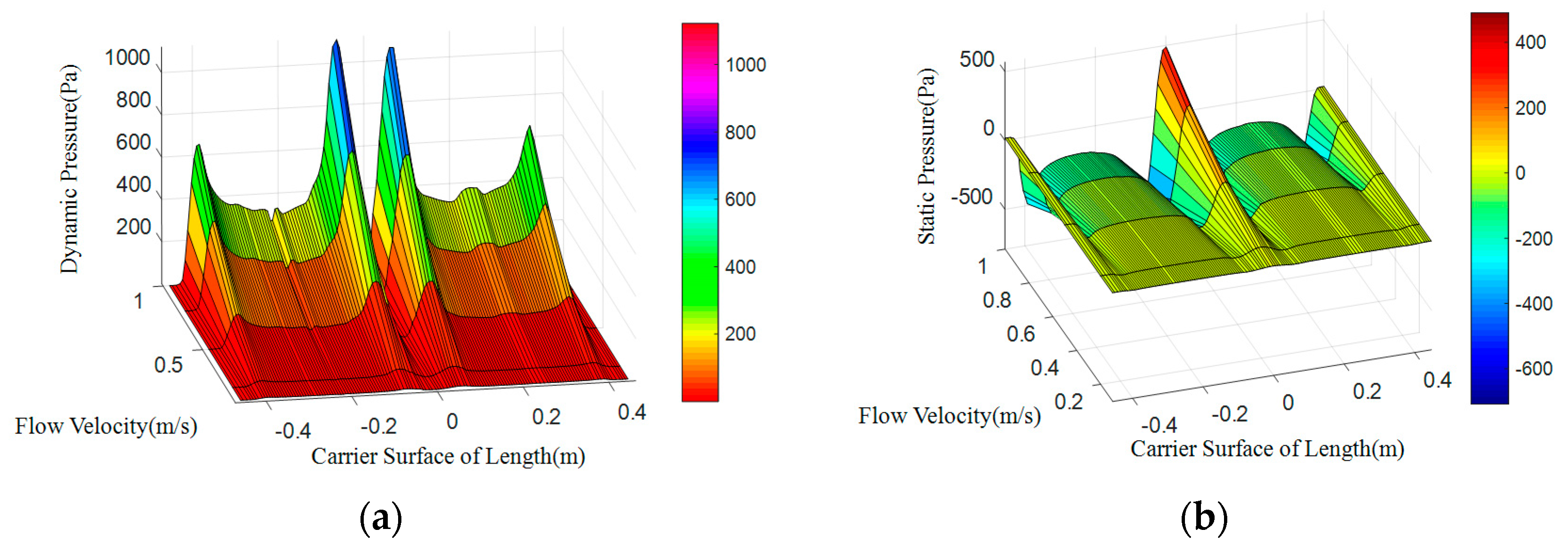
| Extreme Points | Dynamic Pressure | Static Pressure |
|---|---|---|
| Maximum point coordinates | −0.387 | −0.456 0 0.456 |
| −0.066 | ||
| 0.057 | ||
| 0.384 | ||
| Minimum point coordinates | −0.456 0 0.456 | −0.387 |
| −0.066 | ||
| 0.057 | ||
| 0.384 |
| Obstacle Dimensions | Round | Square | |||
|---|---|---|---|---|---|
| Feature size/mm | 50 | 100 | 200 | 300 | 100 (141) |
| Theoretical frequency/Hz | 0.42 | 0.21 | 0.105 | 0.07 | 0.141 |
| Simulation frequency/Hz | 0.4918 | 0.298 | 0.165 | 0.096 | 0.149 |
| Diameter/mm | Main Frequency Peak/Hz | ||
|---|---|---|---|
| 100 | 0.05 | 0.201 | 0.452 |
| 300 | 0.05 | 0.256 | 0.513 |
| Diameter/mm | Theoretical Shedding Frequency/Hz | Simulation Frequency/Hz | Moving Simulation Frequency/Hz | ||
|---|---|---|---|---|---|
| Static | Moving | Static | Moving | ||
| 100 | 0.21 | 0.46 | 0.298 | 0.548 | 0.452 |
| 300 | 0.07 | 0.32 | 0.096 | 0.346 | 0.256 |
| Vibrating FrequencyHz | Pressure Main FrequencyHz | |||
|---|---|---|---|---|
| 0.2 | 0.049 | 0.199 | 0.298 | 0.398 |
| 0.4 | 0.049 | 0.149 | 0.248 | 0.348 |
| 0.6 | 0.149 | 0.248 | 0.348 | 0.447 |
| Item | Parameters |
|---|---|
| Pool size | 1 W × 1.14 (H)(m) |
| Water density | 1.0 × 10³ kg/m3 |
| Experimental water temperature | 18 °C |
| Maximum flow rate | 0.8 m3/s |
| Maximum ideal flow velocity | 0.8 m/s |
| Flow Field | Velocity Estimated Method | Fit Degree |
|---|---|---|
| Uniform | stagnation pressure fitting | 0.9755 |
| static pressure fitting | 0.94–0.96 | |
| Bernoulli method | 0.9925 | |
| turbulent | Karman vortex method | 0.9893 |
| Sensor Pair | Fitness | |
|---|---|---|
| V = 0.3 m/s | V = 0.5 m/s | |
| 6–8 | 0.9856 | 0.9917 |
| 13–11 | 0.9282 | 0.9336 |
| 21–19 | 0.9643 | 0.9811 |
| 22–20 | 0.8534 | 0.9538 |
| Mean | 0.9328 | 0.965 |
| Characteristic Frequency (Hz) | Velocity (m/s) | Calculated Size (mm) | Actual Size (mm) | Error Rate |
|---|---|---|---|---|
| 0.667 | 0.482 | 151.7 | D200 | 24.15% |
| 1.361 | 0.433 | 66.8 | D100 | 33.2% |
| 2.140 | 0.413 | 40.5 | D50 | 19% |
| 0.477 | 0.534 | 235.1 | A200 (282.8) | 16.86% |
| 0.918 | 0.492 | 112.5 | A100 (141.4) | 20.43% |
© 2018 by the authors. Licensee MDPI, Basel, Switzerland. This article is an open access article distributed under the terms and conditions of the Creative Commons Attribution (CC BY) license (http://creativecommons.org/licenses/by/4.0/).
Share and Cite
Liu, G.; Wang, M.; Wang, A.; Wang, S.; Yang, T.; Malekian, R.; Li, Z. Research on Flow Field Perception Based on Artificial Lateral Line Sensor System. Sensors 2018, 18, 838. https://doi.org/10.3390/s18030838
Liu G, Wang M, Wang A, Wang S, Yang T, Malekian R, Li Z. Research on Flow Field Perception Based on Artificial Lateral Line Sensor System. Sensors. 2018; 18(3):838. https://doi.org/10.3390/s18030838
Chicago/Turabian StyleLiu, Guijie, Mengmeng Wang, Anyi Wang, Shirui Wang, Tingting Yang, Reza Malekian, and Zhixiong Li. 2018. "Research on Flow Field Perception Based on Artificial Lateral Line Sensor System" Sensors 18, no. 3: 838. https://doi.org/10.3390/s18030838
APA StyleLiu, G., Wang, M., Wang, A., Wang, S., Yang, T., Malekian, R., & Li, Z. (2018). Research on Flow Field Perception Based on Artificial Lateral Line Sensor System. Sensors, 18(3), 838. https://doi.org/10.3390/s18030838