Single Image Super-Resolution Based on Multi-Scale Competitive Convolutional Neural Network


Abstract
:1. Introduction
- We introduce multi-scale convolutional kernel to traditional convolutional layers, which provides multi-range contextual information for image super-resolution;
- We adopt a competitive strategy to CNN, which not only adaptively choose the optimal scale for convolutional filters but also reduces the dimensionality of the intermediate outputs.
2. Related Work
- corresponds to filters of a size of , where c is the number of image channels and is the spatial size of the filter. The output of the first convolution layer is feature maps to extract and represent each patch as a high-dimensional feature vector.
- The second convolutional layer is responsible for non-linear mapping. Suppose that we obtain dimensional vectors at the above step, the second layer applies filters of size on each feature map. The output -dimensional vectors will be used for reconstruction.
- The last layer is expected to reconstruct the final HR image by recombining the above high-dimensional patch-wise representations.
3. Proposed Method
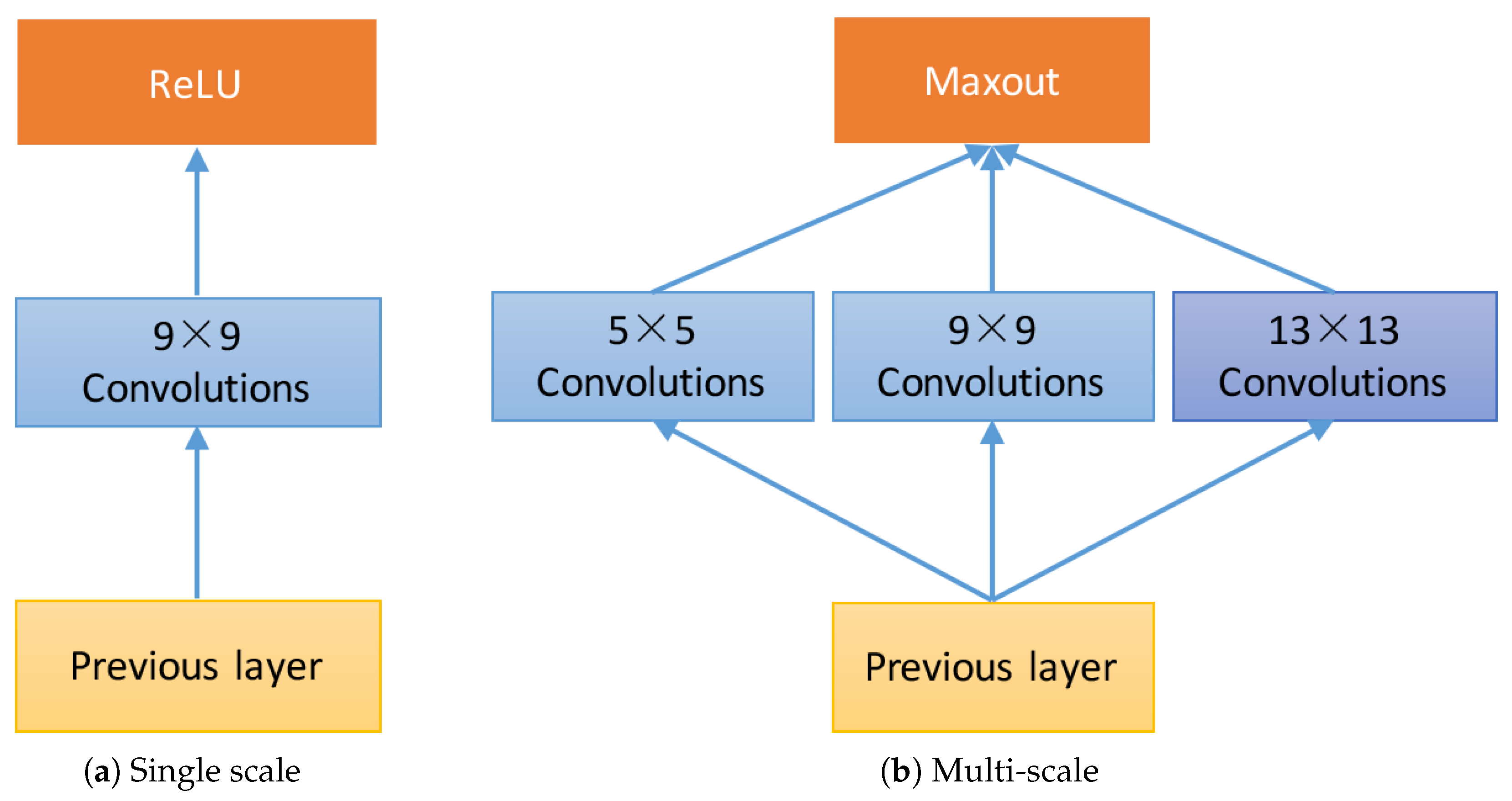
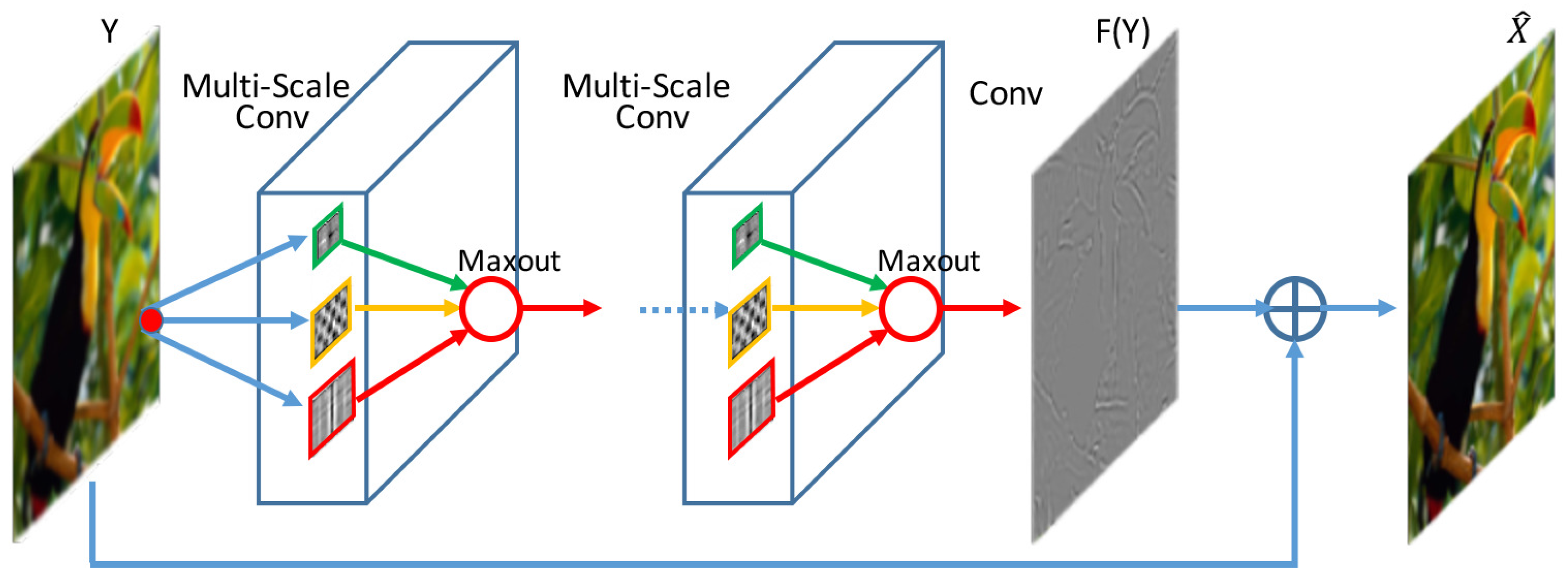
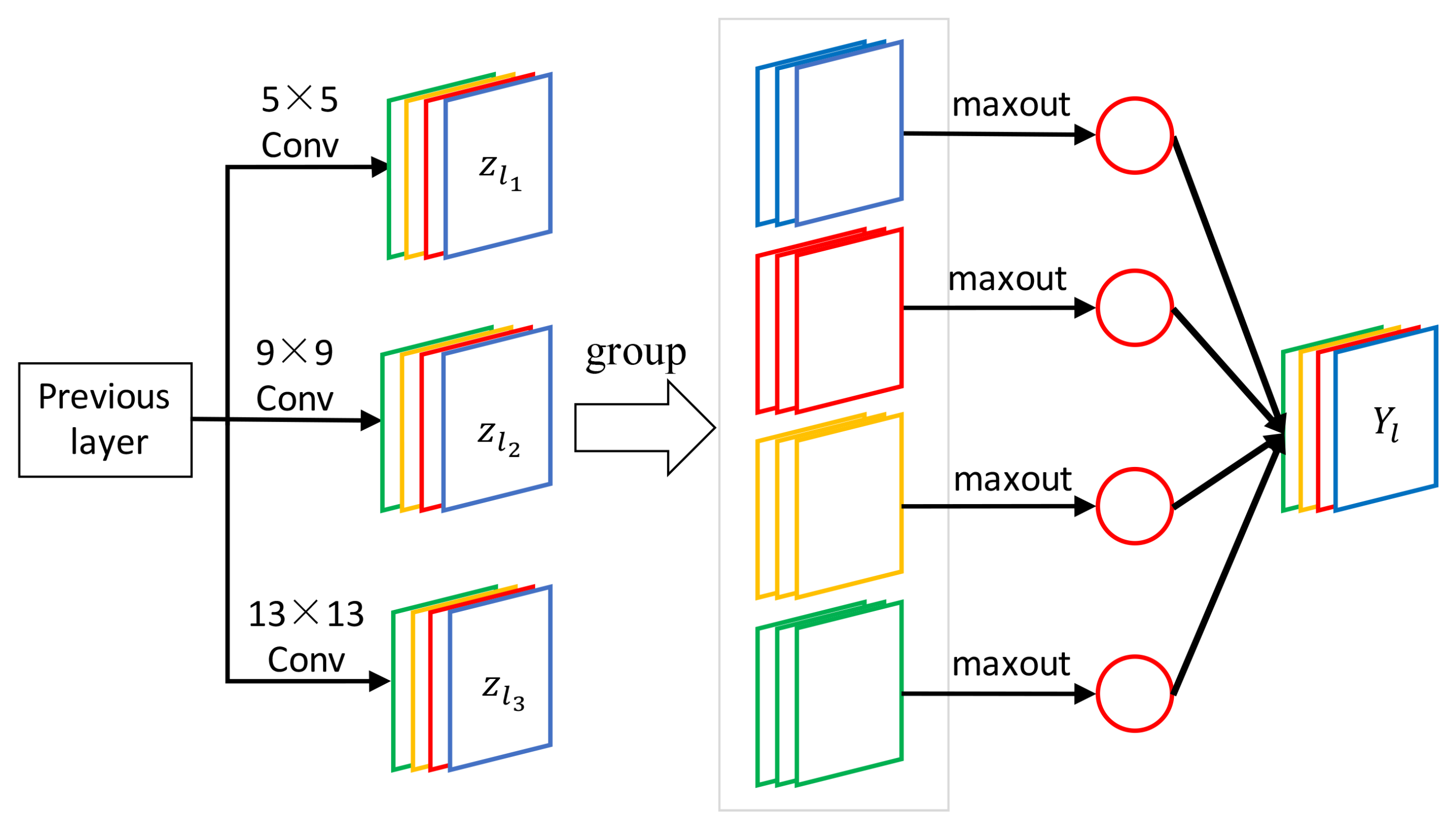
3.1. Multi-scale Competitive Module
- Multi-scale filters are applied on the input image, which produce a set of feature maps to provide different range of image context for image super-resolution. On the contrary, SRCNN only implements single scale receptive field and provides fixed range of contextual information.
- Competitive strategy is introduced to the activation function. The activation function of SRCNN is ReLU, which is replaced by maxout in our network. The maxout unit reduces the dimensionality of the joint filter outputs and promotes competition among the multi-scale filters.
- A shortcut connection with identity mapping is used to add the input image to the output of the last layer. The shortcut connections can effectively facilitate gradient flow through multiple layers. Thus accelerating deep network training [31].
3.2. Training and Prediction
3.2.1. The Loss Function
3.2.2. Training
3.2.3. Prediction
3.3. Model Properties
3.3.1. Multi-Scale Receptive Fields
3.3.2. Competitive Unit Prevents Filter Co-adaptation
3.3.3. Fewer Parameters
4. Experimental Section
4.1. Datasets and Evaluation Criteria
4.2. Parameters and Performance
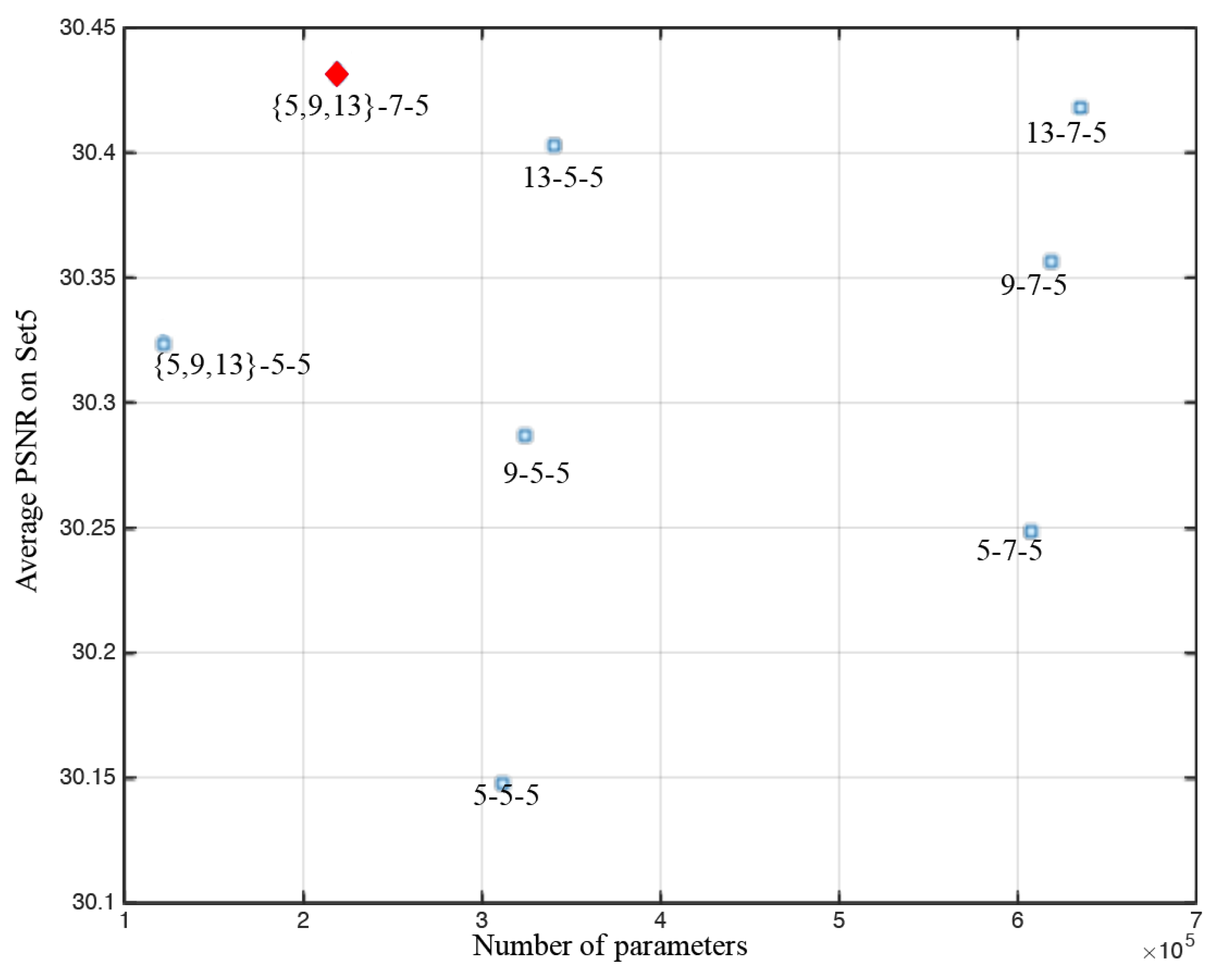
4.2.1. Filter Size and Performance
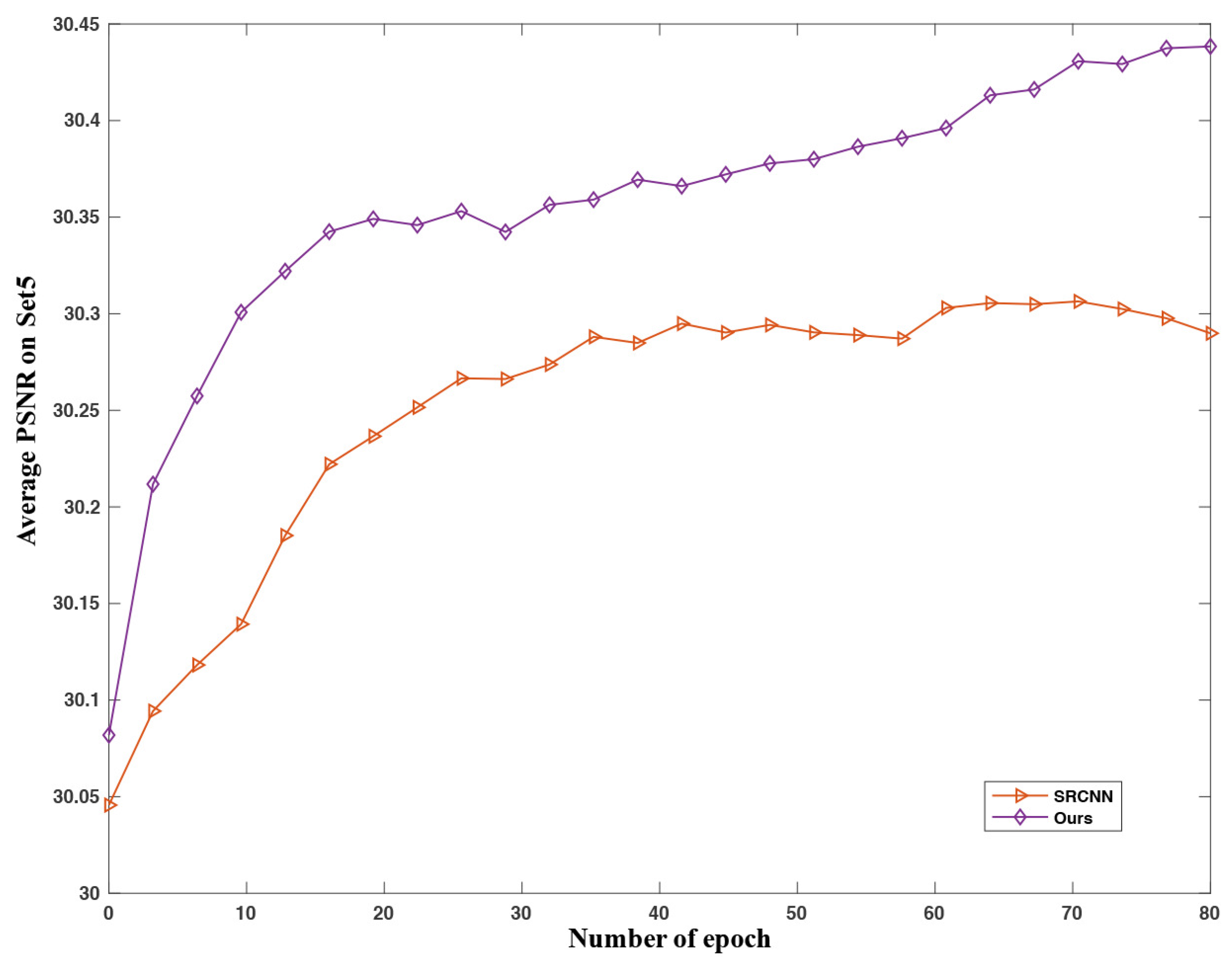
4.2.2. Epoch and Performance
4.3. Results
5. Discussions
5.1. Comparison with Other State-of-Art Methods
5.2. Improvement with Iterative Back Projection
5.3. The Effect of Batch Normalization on Super-Resolution
6. Conclusions
Acknowledgments
Author Contributions
Conflicts of Interest
References
- Nasrollahi, K.; Moeslund, T.B. Super-resolution: A comprehensive survey. Mach. Vis. Appl. 2014, 25, 1423–1468. [Google Scholar] [CrossRef]
- Hou, H.; Andrews, H. Cubic splines for image interpolation and digital filtering. IEEE Trans. Acoust. Speech Signal Process. 1978, 26, 508–517. [Google Scholar]
- Li, X.; Orchard, M.T. New edge-directed interpolation. IEEE Trans. Image Process. 2001, 10, 1521–1527. [Google Scholar] [PubMed]
- Irani, M.; Peleg, S. Improving resolution by image registration. CVGIP: Graph. Models Image Process. 1991, 53, 231–239. [Google Scholar] [CrossRef]
- Efrat, N.; Glasner, D.; Apartsin, A.; Nadler, B.; Levin, A. Accurate blur models vs. image priors in single image super-resolution. In Proceedings of the IEEE International Conference on Computer Vision, Portland, OR, USA, 25–27 June 2013; pp. 2832–2839. [Google Scholar]
- Yang, J.; Wright, J.; Huang, T.; Ma, Y. Image super-resolution as sparse representation of raw image patches. In Proceedings of the IEEE Conference on Computer Vision and Pattern Recognition, Anchorage, AK, USA, 23–28 June 2008; pp. 1–8. [Google Scholar]
- Zheng, H.; Qu, X.; Bai, Z.; Liu, Y.; Guo, D.; Dong, J.; Peng, X.; Chen, Z. Multi-contrast brain magnetic resonance image super-resolution using the local weight similarity. BMC Med. Imaging 2017, 17, 6. [Google Scholar] [CrossRef] [PubMed]
- Wu, J.; Anisetti, M.; Wu, W.; Damiani, E.; Jeon, G. Bayer demosaicking with polynomial interpolation. IEEE Trans. Image Process. 2016, 25, 5369–5382. [Google Scholar] [CrossRef] [PubMed]
- Yang, J.; Wright, J.; Huang, T.S.; Ma, Y. Image super-resolution via sparse representation. IEEE Trans. Image Process. 2010, 19, 2861–2873. [Google Scholar] [CrossRef] [PubMed]
- Timofte, R.; De Smet, V.; Van Gool, L. Anchored neighborhood regression for fast example-based super-resolution. In Proceedings of the IEEE International Conference on Computer Vision, Sydney, Australia, 1–8 December 2013; pp. 1920–1927. [Google Scholar]
- Kim, K.I.; Kwon, Y. Single-image super-resolution using sparse regression and natural image prior. IEEE Trans. Pattern Anal. Mach. Intell. 2010, 32, 1127–1133. [Google Scholar] [PubMed]
- Simonyan, K.; Zisserman, A. Very deep convolutional networks for large-scale image recognition. arXiv, 2014; arXiv:1409.1556. [Google Scholar]
- Rahnemoonfar, M.; Sheppard, C. Deep count: Fruit counting based on deep simulated learning. Sensors 2017, 17, 905. [Google Scholar] [CrossRef] [PubMed]
- Zhang, W.; Zhou, S. DeepMap+: Recognizing high-level indoor semantics using virtual features and samples based on a multi-length window framework. Sensors 2017, 17, 1214. [Google Scholar] [CrossRef] [PubMed]
- Hinton, G.; Deng, L.; Yu, D.; Dahl, G.E.; Mohamed, A.r.; Jaitly, N.; Senior, A.; Vanhoucke, V.; Nguyen, P.; Sainath, T.N.; et al. Deep neural networks for acoustic modeling in speech recognition: The shared views of four research groups. IEEE Signal Process. Mag. 2012, 29, 82–97. [Google Scholar] [CrossRef]
- Dong, C.; Loy, C.C.; He, K.; Tang, X. Image super-resolution using deep convolutional networks. In Proceedings of the IEEE Conference on Computer Vision and Pattern Recognition, Zurich, Switzerland, 6–12 September 2014; pp. 184–199. [Google Scholar]
- Dong, C.; Loy, C.C.; He, K.; Tang, X. Image super-resolution using deep convolutional networks. IEEE Trans. Pattern Anal. Mach. Intell. 2016, 38, 295–307. [Google Scholar] [CrossRef] [PubMed]
- Jain, V.; Seung, S. Natural image denoising with convolutional networks. In Proceedings of the Advances in Neural Information Processing Systems, Vancouver, BC, Canada, 8–10 December 2008; pp. 769–776. [Google Scholar]
- Kim, J.; Lee, J.K.; Lee, K.M. Accurate image super-resolution using very deep convolutional networks. In Proceedings of the IEEE Conference on Computer Vision and Pattern Recognition, Las Vegas, VA, USA, 27–30 June 2016; pp. 1646–1654. [Google Scholar]
- Yamamoto, K.; Togami, T.; Yamaguchi, N. Super-resolution of plant disease images for the acceleration of image-based phenotyping and vigor diagnosis in agriculture. Sensors 2017, 17, 2557. [Google Scholar] [CrossRef] [PubMed]
- Adelson, E.; Simoncelli, E.; Freeman, W.T. Pyramids and multiscale representations. In Representations and Vision; Gorea, A., Ed.; Cambridge University Press: Cambridge, UK, 1991; pp. 3–16. [Google Scholar]
- Mairal, J.; Sapiro, G.; Elad, M. Learning multiscale sparse representations for image and video restoration. Multiscale Model. Simul. 2008, 7, 214–241. [Google Scholar] [CrossRef]
- Arbeláez, P.; Pont-Tuset, J.; Barron, J.T.; Marques, F.; Malik, J. Multiscale combinatorial grouping. In Proceedings of the IEEE Conference on Computer Vision and Pattern Recognition, Columbus, OH, USA, 23–28 June 2014; pp. 328–335. [Google Scholar]
- Yang, X.; Wu, W.; Liu, K.; Chen, W.; Zhang, P.; Zhou, Z. Multi-sensor image super-resolution with fuzzy cluster by using multi-scale and multi-view sparse coding for infrared image. Multimedia Tools Appl. 2017, 76, 24871–24902. [Google Scholar] [CrossRef]
- Yang, X.; Wu, W.; Liu, K.; Chen, W.; Zhou, Z. Multiple dictionary pairs learning and sparse representation-based infrared image super-resolution with improved fuzzy clustering. Soft Comput. 2017. [Google Scholar] [CrossRef]
- Buyssens, P.; Elmoataz, A.; Lézoray, O. Multiscale convolutional neural networks for vision-based classification of cells. In Proceedings of the Asian Conference on Computer Vision, Daejeon, Korea, 5–9 November 2012; pp. 342–352. [Google Scholar]
- Sermanet, P.; LeCun, Y. Traffic sign recognition with multi-scale convolutional networks. In Proceedings of the International Joint Conference on Neural Networks, San Jose, CA, USA, 31 July–5 August 2011; pp. 2809–2813. [Google Scholar]
- Cai, Z.; Fan, Q.; Feris, R.S.; Vasconcelos, N. A unified multi-scale deep convolutional neural network for fast object detection. In Proceedings of the European Conference on Computer Vision, Amsterdam, The Netherlands, 8–16 October 2016; pp. 354–370. [Google Scholar]
- Liao, Z.; Carneiro, G. Competitive multi-scale convolution. arXiv, 2015; arXiv:1511.05635. [Google Scholar]
- Goodfellow, I.J.; Warde-Farley, D.; Mirza, M.; Courville, A.C.; Bengio, Y. Maxout networks. In Proceedings of the 30th International Conference on Machine Learning, Atlanta, GA, USA, 17–19 June 2013; pp. 1319–1327. [Google Scholar]
- He, K.; Zhang, X.; Ren, S.; Sun, J. Deep residual learning for image recognition. In Proceedings of the IEEE Conference on Computer Vision and Pattern Recognition, Seattle, WA, USA, 27–30 June 2016; pp. 770–778. [Google Scholar]
- LeCun, Y.; Bottou, L.; Bengio, Y.; Haffner, P. Gradient-based learning applied to document recognition. Proc. IEEE 1998, 86, 2278–2324. [Google Scholar] [CrossRef]
- Wan, L.; Zeiler, M.; Zhang, S.; Cun, Y.L.; Fergus, R. Regularization of neural networks using dropconnect. In Proceedings of the Machine Learning Research, Atlanta, GA, USA, 17–19 June 2013; pp. 1058–1066. [Google Scholar]
- Martin, D.; Fowlkes, C.; Tal, D.; Malik, J. A database of human segmented natural images and its application to evaluating segmentation algorithms and measuring ecological statistics. In Proceedings of the IEEE International Conference on Computer Vision, Vancouver, BC, Canada, 7–14 July 2001; pp. 416–423. [Google Scholar]
- Vedaldi, A.; Lenc, K. Matconvnet: Convolutional neural networks for matlab. In Proceedings of the ACM International Conference on Multimedia, Brisbane, Australia, 26–30 October 2015; pp. 689–692. [Google Scholar]
- Wang, Z.; Liu, D.; Yang, J.; Han, W.; Huang, T. Deep networks for image super-resolution with sparse prior. In Proceedings of the IEEE International Conference on Computer Vision, Washington, DC, USA, 7–13 December 2015; pp. 370–378. [Google Scholar]
- Dong, C.; Loy, C.C.; Tang, X. Accelerating the super-resolution convolutional neural network. In Proceedings of the European Conference on Computer Vision, Amsterdam, The Netherlands, 8–16 October 2016; pp. 391–407. [Google Scholar]
- Ledig, C.; Theis, L.; Huszar, F.; Caballero, J.; Cunningham, A.; Acosta, A.; Aitken, A.P.; Tejani, A.; Totz, J.; Wang, Z.; et al. Photo-realistic single image super-resolution using a generative adversarial network. In Proceedings of the IEEE Conference on Computer Vision and Pattern Recognition, Honolulu, HI, USA, 21–26 July 2017; pp. 4681–4690. [Google Scholar]
- Shi, W.; Caballero, J.; Huszar, F.; Totz, J.; Aitken, A.P.; Bishop, R.; Rueckert, D.; Wang, Z. Real-time single image and video super-resolution using an efficient sub-pixel convolutional neural network. In Proceedings of the IEEE Conference on Computer Vision and Pattern Recognition, Las Vegas, NV, USA, 27–30 June 2016; pp. 1874–1883. [Google Scholar]
- Dong, C. Image Super-Resolution Using Deep Convolutional Networks. Available online: http://mmlab.ie.cuhk.edu.hk/projects/SRCNN.html (accessed on 20 January 2018).
- Kim, J. Accurate Image Super-Resolution Using Very Deep Convolutional Networks. Available online: https://cv.snu.ac.kr/research/VDSR/ (accessed on 20 January 2018).
- Lim, B.; Son, S.; Kim, H.; Nah, S.; Lee, K.M. Enhanced eeep residual networks for single image super-Resolution. In Proceedings of the IEEE Conference on Computer Vision and Pattern Recognition Workshops, Honolulu, HI, USA, 21–26 July 2017; pp. 1132–1140. [Google Scholar]


| Network | Parameter Number |
|---|---|
| 9-5-5 | 324,352 |
| 13-7-5 | 636,160 |
| {5,9,13}-5-5 | 123,600 |
| {5,9,13}-7-5 | 219,904 |
| Time | SRCNN (9-5-5) | Ours ({5,9,13}-7-5) |
|---|---|---|
| Training with GPU (one epoch) | 12 min | 15 min |
| Prediction with CPU () | 0.30 s | 0.56 s |
| Network | SRCNN (9-5-5) | Ours ({5,9,13}-7-5) |
|---|---|---|
| Amount of parameters | 224 KB | 465 KB |
| Memory cost (training) | 24 MB | 64 MB |
| Memory cost (prediction) | 49 MB | 129 MB |
| Proposed Method | PSNR |
|---|---|
| {3,5,9}-7-5 | 30.10 |
| {5,9,13}-7-5 | 30.44 |
| {7,9,13}-7-5 | 30.44 |
| {5,11,13}-7-5 | 30.43 |
| {7,9,15}-7-5 | 30.33 |
| {7,13,15}-7-5 | 30.27 |
| Dataset Upscaling Factor | Set5 2 | Set14 2 | Set5 3 | Set14 3 | Set5 4 | Set14 4 |
|---|---|---|---|---|---|---|
| Bicubic | 33.66/0.9299 | 30.33/0.8694 | 30.39/0.8681 | 27.61/0.7752 | 28.42/0.8104 | 26.06/0.7042 |
| A+ | 35.95/0.9508 | 31.84/0.9017 | 32.07/0.8984 | 28.71/0.8121 | 29.83/0.8465 | 27.02/0.7421 |
| SRCNN | 36.66/0.9542 | 32.55/0.9073 | 32.75/0.9090 | 29.39/0.8225 | 30.49/0.8628 | 27.60/0.7529 |
| CSCN | 36.93/0.9552 | 32.56/0.9074 | 33.10/0.9144 | 29.41/0.8238 | 30.86/0.8732 | 27.64/0.7578 |
| FSRCNN | 37.00/0.9558 | 32.63/0.9088 | 33.16/0.9140 | 29.43/0.8242 | 30.71/0.8657 | 27.59/0.7535 |
| Ours (shallow) | 37.03/0.9566 | 32.69/0.9103 | 33.04/0.9140 | 29.43/0.8258 | 30.72/0.8706 | 27.68/0.7581 |
| Ours (deep) | 37.23/0.9575 | 32.73/0.9222 | 33.44/0.9185 | 29.58/0.8290 | 31.10/0.8785 | 27.79/0.7627 |
| Bicubic | A+ | SRCNN | Ours (Shallow) | Ours (Deep) | |
|---|---|---|---|---|---|
| Image | PSNR/SSIM | PSNR/SSIM | PSNR/SSIM | PSNR/SSIM | PSNR/SSIM |
| baby | 31.78/0.8567 | 33.07/0.8811 | 33.13/0.8824 | 32.75/0.8807 | 33.06/0.8824 |
| bird | 30.18/0.8729 | 32.03/0.9048 | 32.52/0.9112 | 32.76/0.9163 | 33.22/0.9232 |
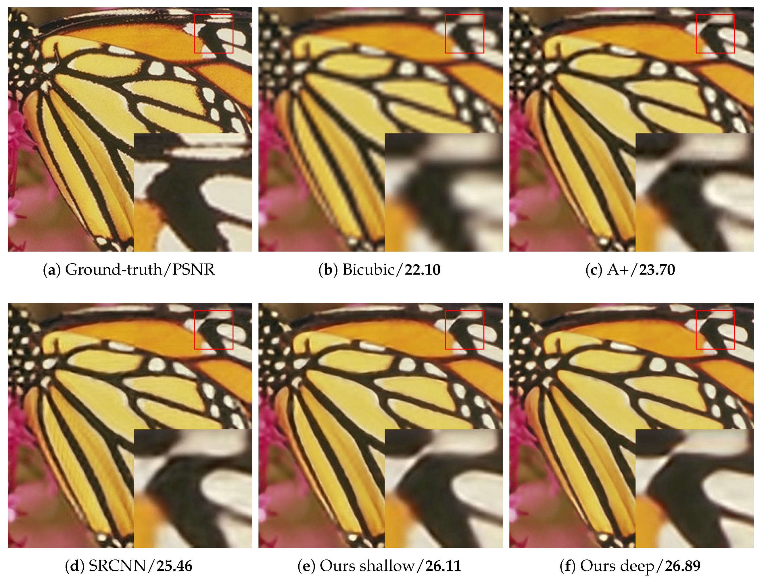
| butterfly | 22.10/0.7369 | 23.70/0.8023 | 25.46/0.8566 | 26.11/0.8801 | 26.89/0.8987 |
| head | 31.59/0.7536 | 32.30/0.7771 | 32.44/0.7801 | 32.49/0.7836 | 32.67/0.7884 |
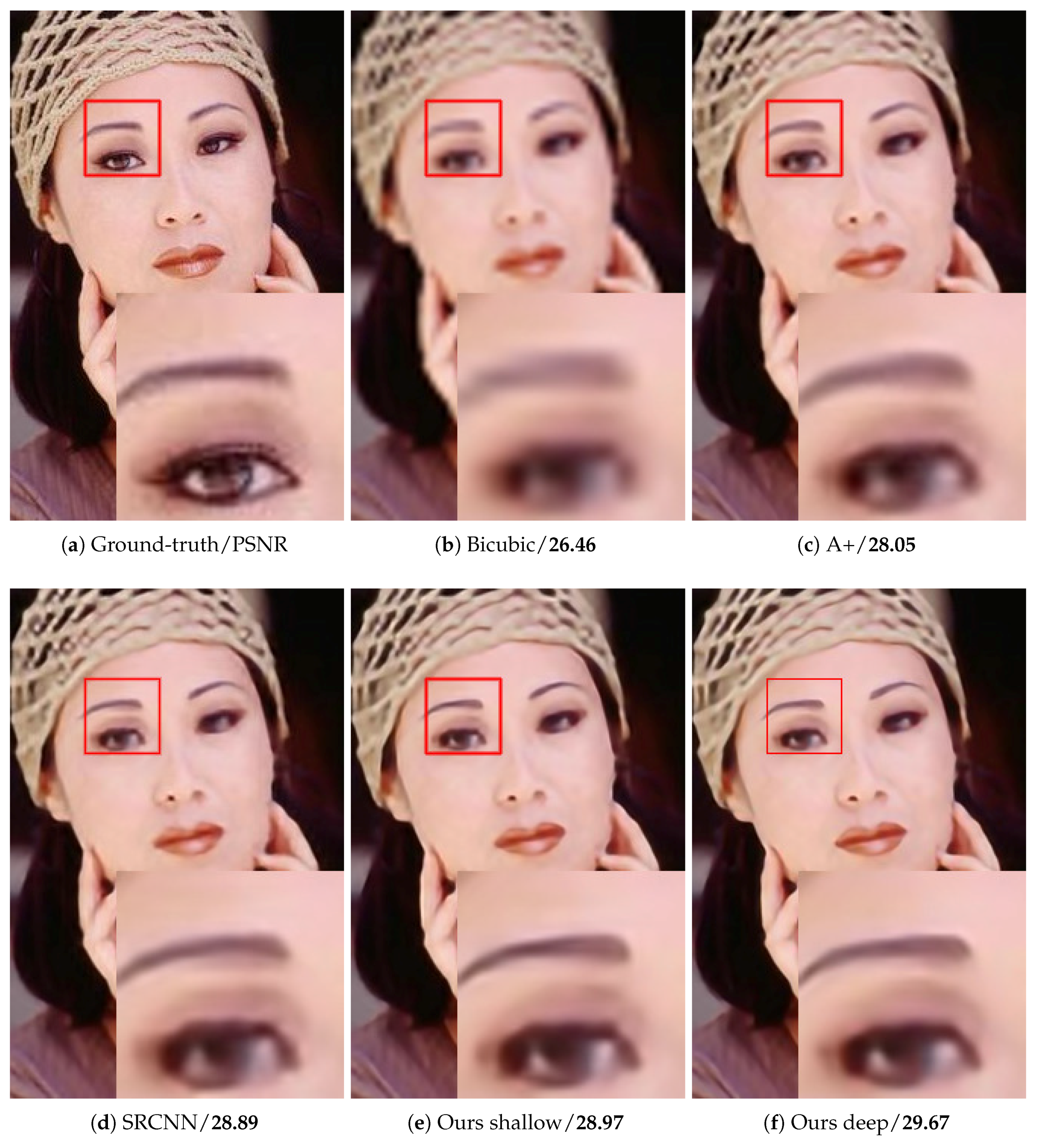
| woman | 26.46/0.8318 | 28.05/0.8670 | 28.89/0.8837 | 28.97/0.8893 | 29.67/0.8996 |
| baboon | 22.41/0.4521 | 22.71/0.5002 | 22.73/0.5029 | 22.76/0.5112 | 22.80/0.5128 |
| barbara | 25.17/0.6873 | 25.68/0.7245 | 25.76/0.7293 | 25.74/0.7346 | 25.94/0.7413 |
| bridge | 24.44/0.5652 | 24.01/0.6233 | 25.11/0.6220 | 25.17/0.6288 | 25.28/0.6332 |
| coastguard | 25.38/0.5238 | 25.80/0.5539 | 26.04/0.5563 | 26.09/0.5623 | 26.16/0.5667 |
| comic | 21.72/0.5852 | 22.41/0.6454 | 22.70/0.6658 | 22.76/0.6773 | 22.88/0.6864 |
| face | 31.60/0.753 | 32.27/0.7757 | 32.38/0.7779 | 32.42/0.7808 | 32.61/0.7862 |
| flowers | 25.59/0.7233 | 26.62/0.7648 | 27.14/0.7791 | 27.21/0.7856 | 27.20/0.7901 |
| foreman | 28.79/0.8625 | 31.22/0.8927 | 32.14/0.9080 | 32.14/0.9109 | 32.30/0.9146 |
| lenna | 29.87/0.8149 | 31.18/0.8416 | 31.41/0.8436 | 31.51/0.8481 | 31.79/0.8522 |
| man | 25.72/0.6760 | 26.52/0.7182 | 26.89/0.7300 | 27.00/0.7370 | 27.14/0.7428 |
| monarch | 27.51/0.8817 | 28.88/0.9037 | 30.22/0.9181 | 30.76/0.9251 | 31.35/0.9312 |
| pepper | 30.42/0.8359 | 32.28/0.8583 | 32.98/0.8648 | 32.95/0.8674 | 33.48/0.8720 |
| ppt3 | 22.04/0.8151 | 23.06/0.8473 | 24.80/0.8928 | 24.27/0.8871 | 23.66/0.8867 |
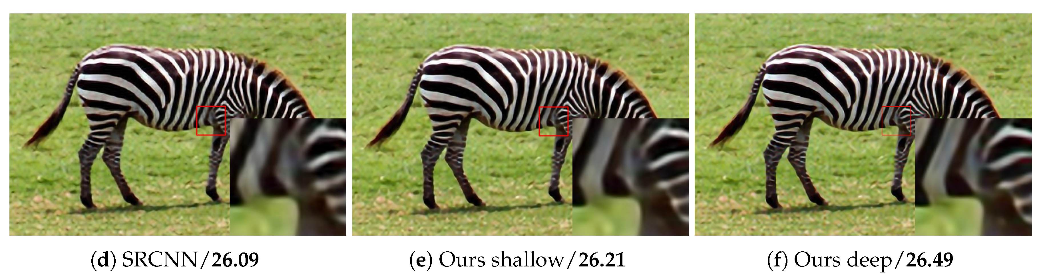
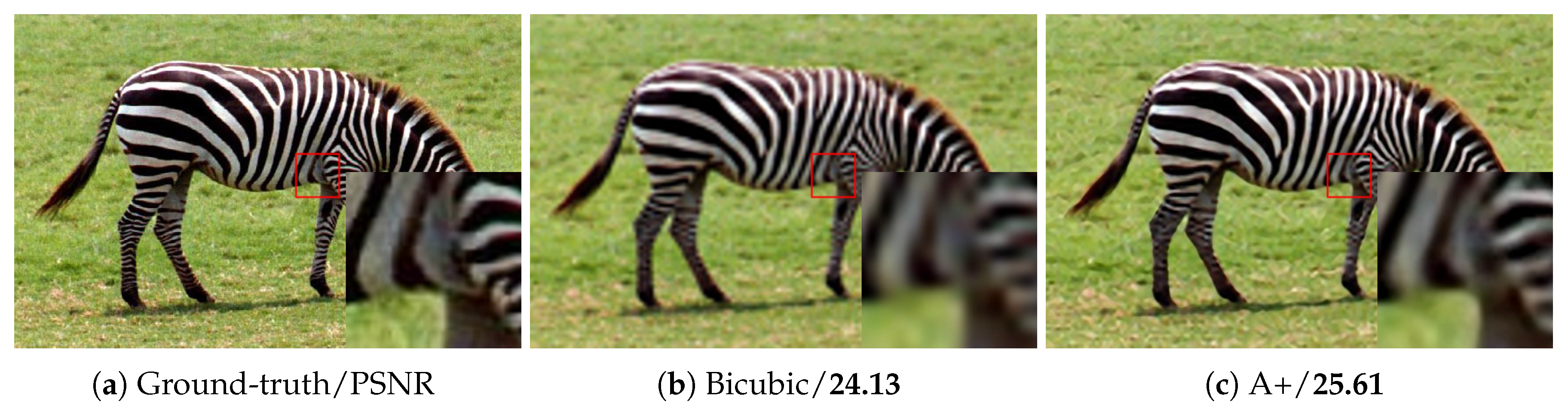
| zebra | 24.13/0.6831 | 25.61/0.7391 | 26.09/0.7505 | 26.21/0.7605 | 26.49/0.7615 |
| Dataset | Upscaling | Shallow Network | Much Deeper Network | |||
|---|---|---|---|---|---|---|
| Factor | Proposed Method | SRCNN | ESPCN | SRGAN | VDSR | |
| BSD300 | 2 | 31.62 | 31.31 | N/A | N/A | 31.90 |
| 3 | 28.60 | 28.37 | 28.54 | N/A | 28.82 | |
| 4 | 27.07 | 26.87 | 27.06 | 25.16 | 27.29 | |
| BSD500 | 2 | 31.95 | 31.58 | N/A | N/A | 32.27 |
| 3 | 28.72 | 28.45 | 28.64 | N/A | 28.95 | |
| 4 | 27.10 | 26.90 | 27.07 | N/A | 27.31 | |
| Set5 | 2 | 37.23 | 36.66 | N/A | N/A | 37.53 |
| 3 | 33.44 | 32.75 | 33.13 | N/A | 33.66 | |
| 4 | 31.10 | 30.49 | 30.90 | 29.40 | 31.35 | |
| Set14 | 2 | 32.73 | 32.55 | N/A | N/A | 33.03 |
| 3 | 29.58 | 29.39 | 29.49 | N/A | 29.77 | |
| 4 | 27.79 | 27.60 | 27.73 | 26.02 | 28.01 | |
| Upscaling | Proposed Method | ||
|---|---|---|---|
| Factor | Dateset | Without IBP | With IBP |
| 2 | Set5 | 37.23/0.9575 | 37.28/0.9579 |
| Set14 | 32.73/0.9222 | 32.89/0.9110 | |
| 3 | Set5 | 33.44/0.9185 | 33.53/0.9195 |
| Set14 | 29.58/0.8290 | 29.70/0.8296 | |
| 4 | Set5 | 31.10/0.8785 | 31.19/0.8800 |
| Set14 | 27.79/0.7627 | 27.86/0.7632 | |
| Upscaling | Proposed Method | ||
|---|---|---|---|
| Factor | Dateset | Without BN | With BN |
| 2 | Set5 | 37.03/0.9566 | 36.90/0.9556 |
| Set14 | 32.69/0.9103 | 32.62/0.9087 | |
| 3 | Set5 | 33.04/0.9140 | 32.88/0.9117 |
| Set14 | 29.43/0.8258 | 29.35/0.8236 | |
| 4 | Set5 | 30.72/0.8706 | 30.56/0.8663 |
| Set14 | 27.68/0.7581 | 27.59/0.7542 | |
© 2018 by the authors. Licensee MDPI, Basel, Switzerland. This article is an open access article distributed under the terms and conditions of the Creative Commons Attribution (CC BY) license (http://creativecommons.org/licenses/by/4.0/).
Share and Cite
Du, X.; Qu, X.; He, Y.; Guo, D. Single Image Super-Resolution Based on Multi-Scale Competitive Convolutional Neural Network. Sensors 2018, 18, 789. https://doi.org/10.3390/s18030789
Du X, Qu X, He Y, Guo D. Single Image Super-Resolution Based on Multi-Scale Competitive Convolutional Neural Network. Sensors. 2018; 18(3):789. https://doi.org/10.3390/s18030789
Chicago/Turabian StyleDu, Xiaofeng, Xiaobo Qu, Yifan He, and Di Guo. 2018. "Single Image Super-Resolution Based on Multi-Scale Competitive Convolutional Neural Network" Sensors 18, no. 3: 789. https://doi.org/10.3390/s18030789
APA StyleDu, X., Qu, X., He, Y., & Guo, D. (2018). Single Image Super-Resolution Based on Multi-Scale Competitive Convolutional Neural Network. Sensors, 18(3), 789. https://doi.org/10.3390/s18030789