ISBDD Model for Classification of Hyperspectral Remote Sensing Imagery


 ,
,
Abstract
1. Introduction
2. Materials and Methods
2.1. DD Algorithm
2.2. Classification of Hyperspectral Remotely Sensed Image Based on the DD Algorithm
2.3. ISBDD Model for Classification of Hyperspectral Remotely Sensed Image
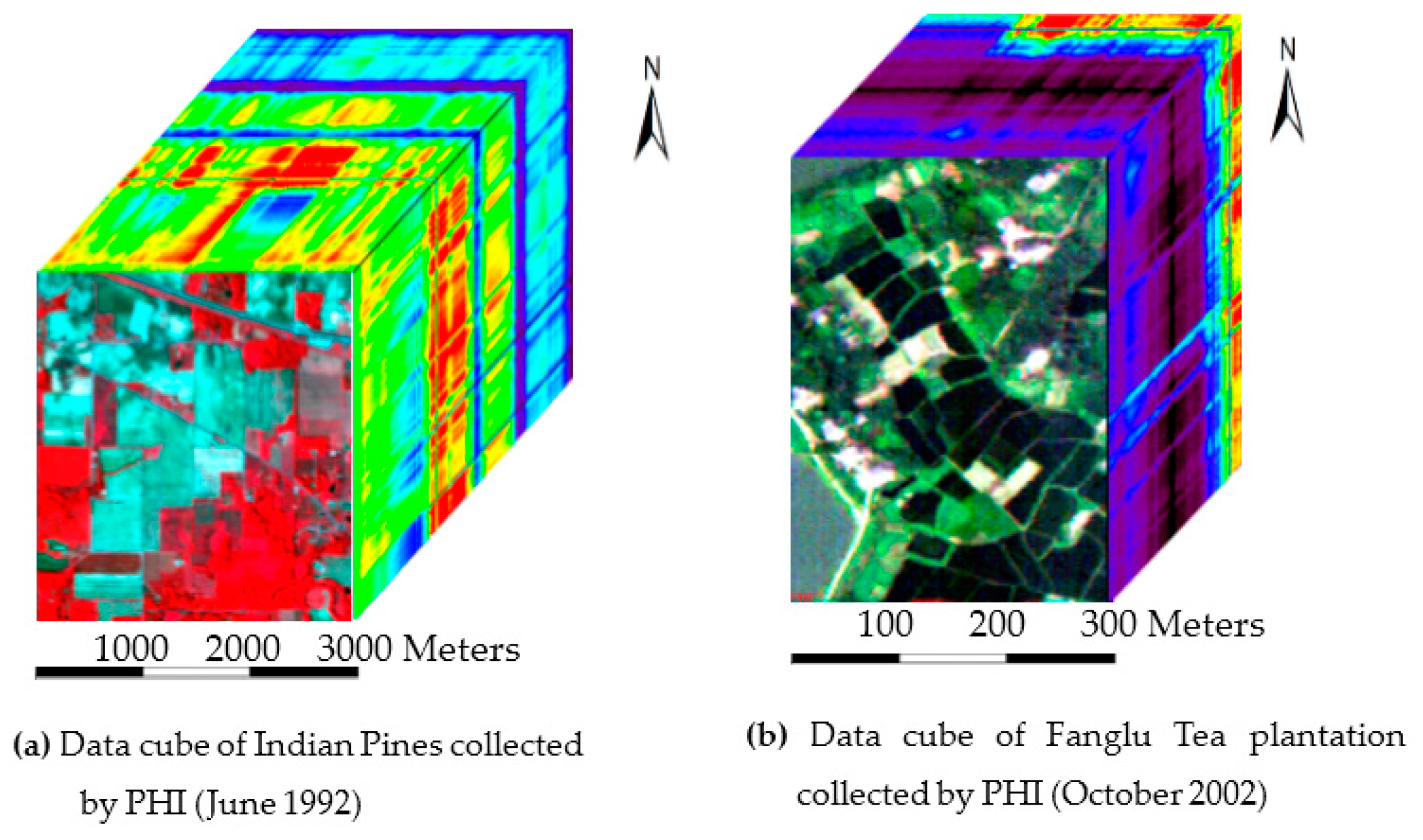
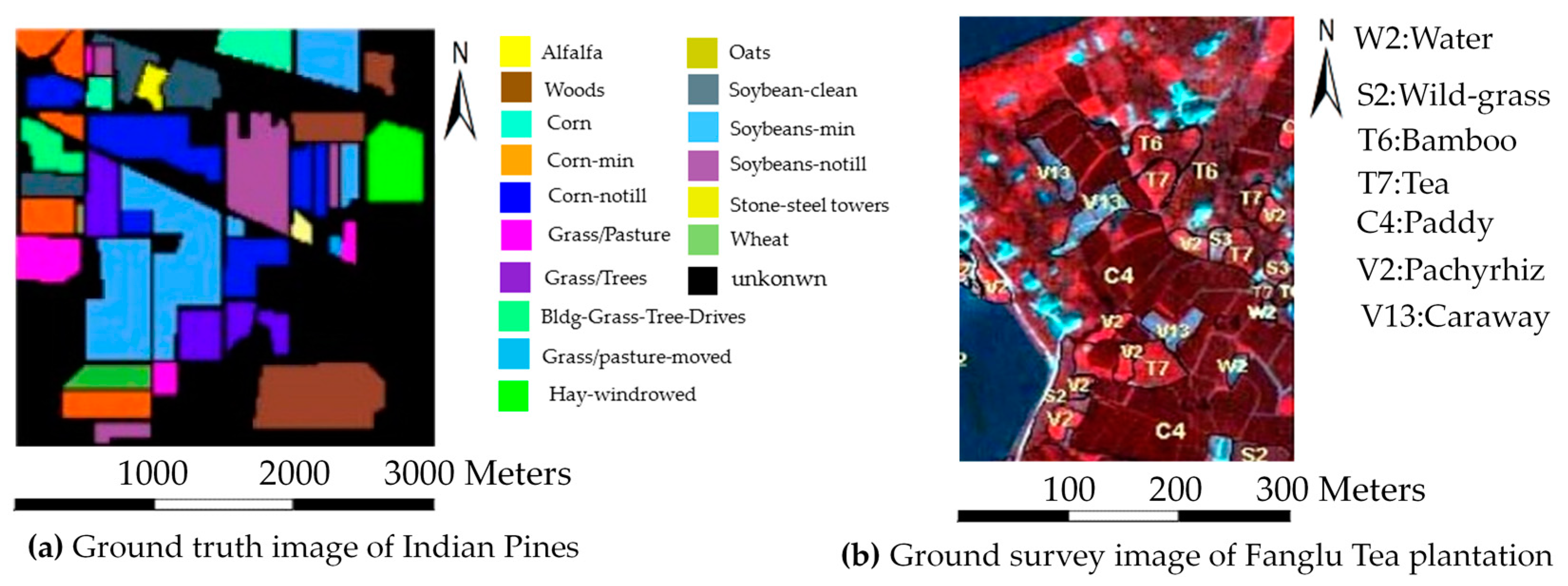
2.4. Experiment Description
3. Results
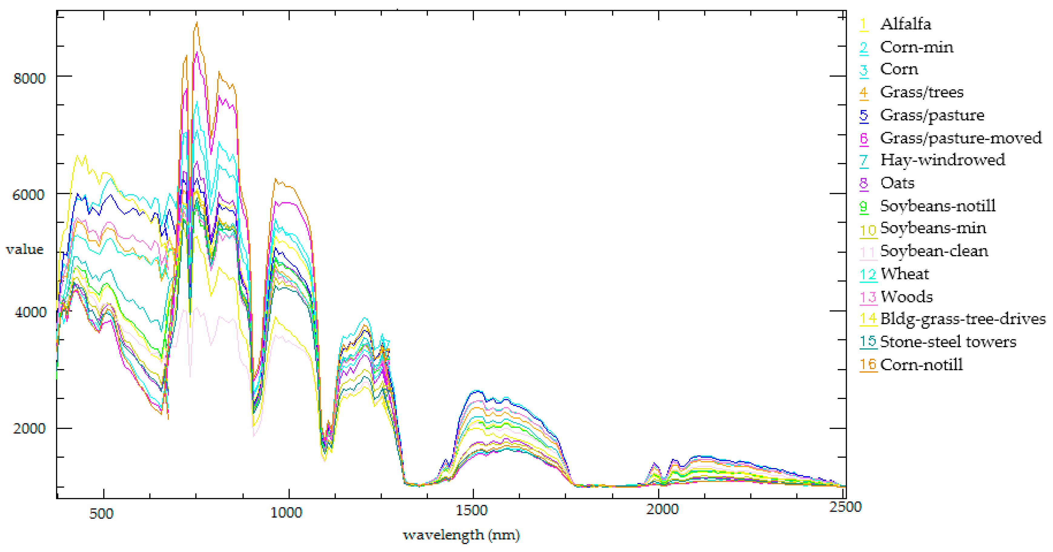
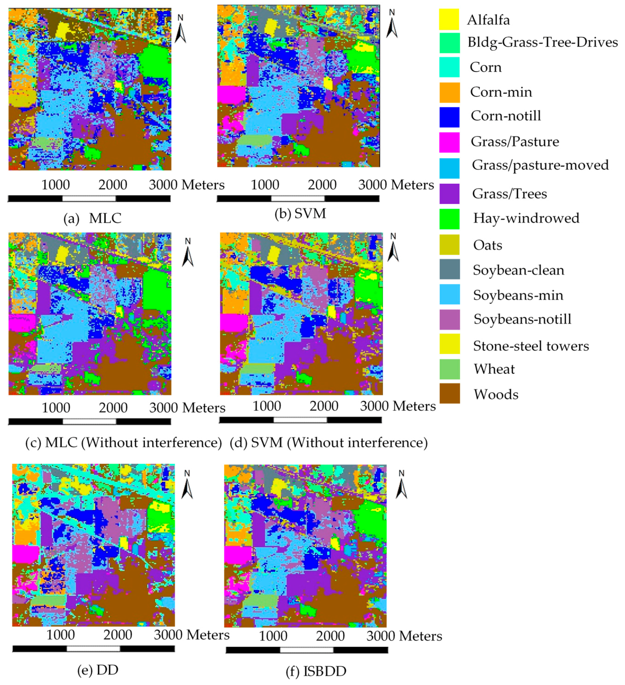
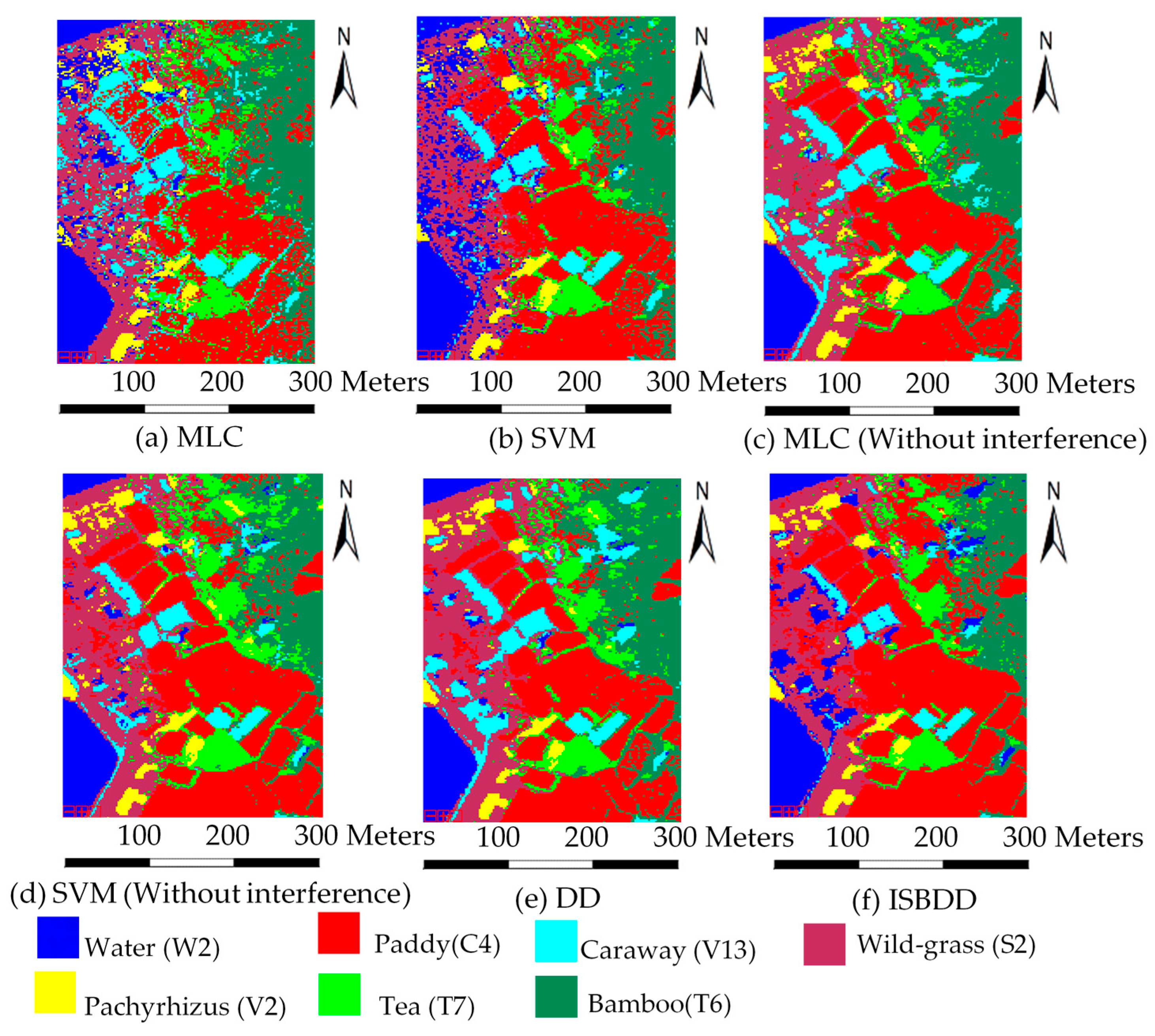
3.1. AVIRIS Image
3.2. PHI Image
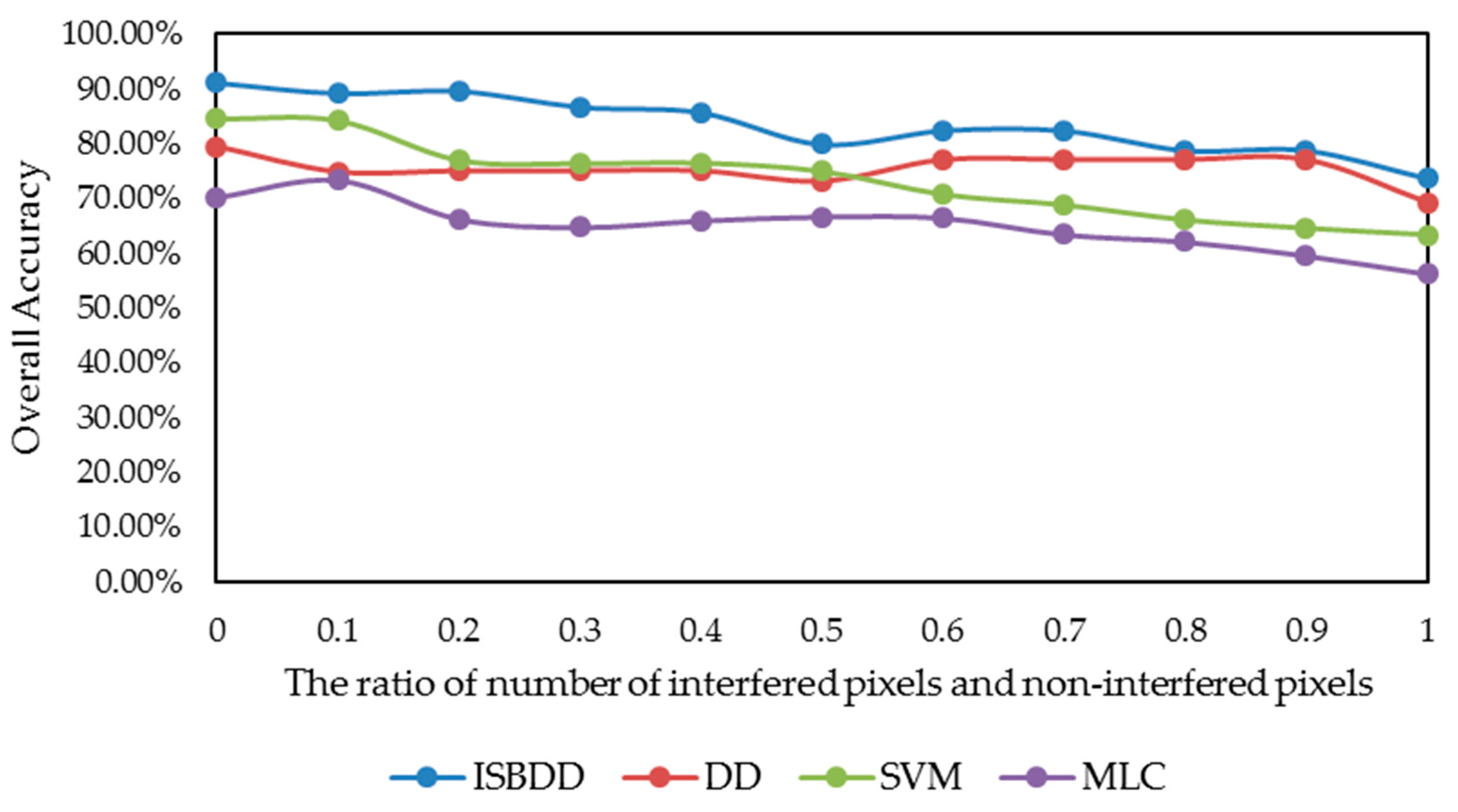
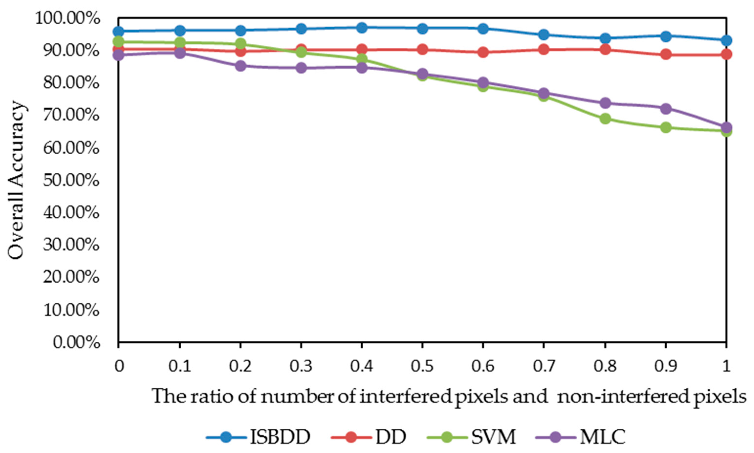
4. Discussion
4.1. Influence of Interference Intensity
4.2. Application Prospects and Future Work
5. Conclusions
Acknowledgments
Author Contributions
Conflicts of Interest
References
- Garaba, S.P.; Zielinski, O. Comparison of remote sensing reflectance from above-water and in-water measurements west of Greenland, Labrador Sea, Denmark Strait, and west of Iceland. Opt. Express 2013, 21, 15938–15950. [Google Scholar] [CrossRef] [PubMed]
- Filippi, A.M.; Archibald, R.; Bhaduri, B.L.; Bright, E.A. Hyperspectral agricultural mapping using support vector machine-based endmember extraction (SVM-BEE). Opt. Express 2009, 17, 23823–23842. [Google Scholar] [CrossRef] [PubMed]
- Babaeian, E.; Homaee, M.; Montzka, C.; Vereecken, H.; Norouzi, A.A. Towards retrieving soil hydraulic properties by hyperspectral remote sensing. Vadose Zone J. 2015, 14. [Google Scholar] [CrossRef]
- Klein, M.E.; Aalderink, B.J.; Padoan, R.; De Bruin, G.; Steemers, T.A. Quantitativen Hyperspectral Reflectance Imaging. Sensors 2008, 8, 5576–5618. [Google Scholar] [CrossRef] [PubMed]
- Jia, X.; Kuo, B.C.; Crawford, M.M. Feature mining for hyperspectral image classification. Proc. IEEE 2013, 101, 676–697. [Google Scholar] [CrossRef]
- Qi, B.; Zhao, C.; Youn, E.; Nansen, C. Use of weighting algorithms to improve traditional support vector machine based classifications of reflectance data. Opt. Express 2011, 19, 26816–26826. [Google Scholar] [CrossRef] [PubMed]
- Li, N.; Cao, Y. An improved classification approach based on spatial and spectral features for hyperspectral data. Spectrosc. Spectr. Anal. 2014, 34, 526–531. [Google Scholar]
- Li, N.; Zhao, H.J.; Huang, P.; Jia, G.R.; Bai, X. A novel logistic multi-Class supervised classification model based on multi-fractal spectrum parameters for hyperspectral Data. Int. J. Comput. Math. 2015, 92, 836–849. [Google Scholar] [CrossRef]
- Tao, D.; Jia, G.; Yuan, Y.; Zhao, H. A digital sensor simulator of the pushbroom offner hyperspectral imaging spectrometer. Sensors 2014, 14, 23822–23842. [Google Scholar] [CrossRef] [PubMed]
- Dietterich, T.G.; Lathrop, R.H.; Lozano-Pérez, T. Solving the multiple instance problem with axis-parallel rectangles. Artif. Intell. 1997, 89, 31–71. [Google Scholar] [CrossRef]
- Maron, O.; Lozano-Pérez, T. A framework for multiple-instance learning. Adv. Neural Inf. Process. Syst. 1998, 200, 570–576. [Google Scholar]
- Du, P.; Samat, A. Multiple instance learning method for high-resolution remote sensing image classification. Remote Sens. Inf. 2012, 27, 60–66. [Google Scholar]
- Wada, T.; Mukai, Y. Fast Keypoint Reduction for Image Retrieval by Accelerated Diverse Density Computation. In Proceedings of the 2015 IEEE International Conference on Data Mining Workshop, Atlantic City, NJ, USA, 14–17 November 2015; pp. 102–107. [Google Scholar]
- Bolton, J.; Gader, P. Application of Multiple-Instance Learning for Hyperspectral Image Analysis. IEEE Geosci. Remote Sens. Lett. 2015, 8, 889–893. [Google Scholar] [CrossRef]
- Bolton, J.; Gader, P. Multiple instance learning for hyperspectral image analysis. In Proceedings of the 2010 IEEE International Geoscience and Remote Sensing Symposium (IGARSS), Honolulu, HI, USA, 25–30 July 2010; pp. 4232–4235. [Google Scholar]
- Bolton, J.; Gader, P. Spatial multiple instance learning for hyperspectral image analysis. In Proceedings of the 2010 2nd Workshop on Hyperspectral Image and Signal Processing: Evolution in Remote Sensing, Reykjavik, Iceland, 14–16 June 2010; Volume 8, pp. 1–4. [Google Scholar]
- Vanwinckelen, G.; Fierens, D.; Blockeel, H. Instance-level accuracy versus bag-level accuracy in multi-instance learning. Data Min. Knowl. Discov. 2016, 30, 313–341. [Google Scholar] [CrossRef]
- Xu, L.; Guo, M.Z.; Zou, Q.; Liu, Y.; Li, H.F. An Improved Diverse Density Algorithm for Multiple Overlapped Instances. In Proceedings of the Fourth International Conference on Natural Computation (ICNC ’08), Jinan, China, 18–20 October 2008. [Google Scholar]
- Fu, J.; Yin, J. Bag-level active multi-instance learning. In Proceedings of the Eighth International Conference on Fuzzy Systems and Knowledge Discovery (FSKD), Shanghai, China, 26–28 July 2011; Volume 2, pp. 1307–1311. [Google Scholar]
- Chen, M.S.; Yang, S.Y.; Zhao, Z.J.; Fu, P.; Sun, Y.; Li, X.; Sun, Y.; Qi, X. Multi-points diverse density learning algorithm and its application in image retrieval. J. Jilin Univ. 2011, 41, 1456–1460. [Google Scholar]
- Ordóñez, C.; Cabo, C.; Sanz-Ablanedo, E. Automatic Detection and Classification of Pole-Like Objects for Urban Cartography Using Mobile Laser Scanning Data. Sensors 2017, 17, 1465. [Google Scholar] [CrossRef] [PubMed]
- Kozoderov, V.V.; Dmitriev, E.V. Testing different classification methods in airborne hyperspectral imagery processing. Opt. Express 2016, 24, A956–A965. [Google Scholar] [CrossRef] [PubMed]


| Class ID | Class Name | Training Samples | Testing Samples | |
|---|---|---|---|---|
| Without Interference | With Interference | |||
| 1 | Alfalfa | 25 | 32 | 18 |
| 2 | Corn-min | 28 | 35 | 81 |
| 3 | Corn | 30 | 38 | 54 |
| 4 | Grass/trees | 31 | 40 | 161 |
| 5 | Grass/pasture | 25 | 30 | 80 |
| 6 | Grass/pasture-moved | 20 | 25 | 12 |
| 7 | Hay-windrowed | 50 | 65 | 64 |
| 8 | Oats | 20 | 25 | 10 |
| 9 | Soybeans-notill | 29 | 37 | 155 |
| 10 | Soybeans-min | 39 | 53 | 184 |
| 11 | Soybean-clean | 38 | 48 | 75 |
| 12 | Wheat | 30 | 40 | 60 |
| 13 | Woods | 38 | 48 | 156 |
| 14 | Bldg-grass-tree-drives | 30 | 25 | 60 |
| 15 | Stone-steel towers | 35 | 45 | 16 |
| 16 | Corn-notill | 30 | 38 | 178 |
| Class ID | Class Name | Training Samples | Testing Samples | |
|---|---|---|---|---|
| Without Interference | With Interference | |||
| 1(W2) | Water | 92 | 120 | 954 |
| 2(C4) | Paddy | 195 | 255 | 976 |
| 3(V13) | Caraway | 105 | 138 | 295 |
| 4(S2) | Wild-grass | 105 | 135 | 382 |
| 5(V2) | Pachyrhizus | 66 | 82 | 211 |
| 6(T7) | Tea | 105 | 135 | 411 |
| 7(T6) | Bamboo | 135 | 180 | 443 |
| Method | MLC | SVM | MLC (Without Interference) | SVM (Without Interference) | DD | ISBDD |
|---|---|---|---|---|---|---|
| Alfalfa (%) | 85.56 | 100.0 | 81.11 | 100.00 | 100.0 | 100.0 |
| Corn-min (%) | 56.22 | 67.55 | 66.71 | 96.22 | 77.20 | 91.19 |
| Corn (%) | 97.14 | 98.57 | 97.14 | 98.57 | 24.29 | 75.71 |
| Grass/trees (%) | 60.40 | 75.30 | 79.06 | 99.73 | 91.41 | 95.70 |
| Grass/pasture (%) | 81.00 | 100.0 | 87.17 | 100.00 | 100.0 | 100.0 |
| Grass/pasture-moved (%) | 63.33 | 100.0 | 11.67 | 100.00 | 100.0 | 100.0 |
| Hay-windrowed (%) | 99.87 | 90.67 | 99.87 | 89.87 | 77.74 | 89.87 |
| Oats (%) | 24.00 | 92.00 | 8.00 | 100.00 | 88.00 | 100.0 |
| Soybeans-notill (%) | 32.39 | 57.32 | 28.31 | 56.34 | 77.32 | 76.62 |
| Soybeans-min (%) | 78.16 | 88.78 | 88.57 | 85.30 | 77.96 | 94.90 |
| Soybean-clean (%) | 100.0 | 100.0 | 100.00 | 100.00 | 93.21 | 100.0 |
| Wheat (%) | 95.67 | 100.0 | 97.33 | 100.00 | 100.0 | 100.0 |
| Woods (%) | 98.10 | 99.05 | 98.33 | 99.29 | 93.33 | 100.0 |
| Bldg-grass-tree-drives (%) | 11.00 | 34.33 | 7.33 | 39.67 | 50.67 | 59.00 |
| Stone-steel towers (%) | 100.0 | 100.0 | 100.00 | 98.40 | 29.60 | 99.20 |
| Corn-notill (%) | 40.95 | 35.81 | 18.86 | 47.43 | 60.57 | 65.52 |
| Overall accuracy (%) | 68.17 | 77.74 | 69.92 | 84.75 | 80.55 | 89.02 |
| Kappa coefficient | 0.65 | 0.76 | 0.67 | 0.84 | 0.79 | 0.88 |
| Method | MLC | SVM | MLC (Without Interference) | SVM (Without Interference) | DD | ISBDD |
|---|---|---|---|---|---|---|
| Water (%) | 92.24 | 95.66 | 91.72 | 94.32 | 93.27 | 97.72 |
| Paddy (%) | 69.45 | 80.00 | 82.09 | 98.07 | 71.74 | 99.78 |
| Caraway (%) | 98.37 | 98.10 | 100.00 | 99.46 | 99.52 | 98.85 |
| Wild-grass (%) | 79.58 | 72.09 | 92.98 | 94.56 | 96.65 | 92.20 |
| Pachyrhizus (%) | 88.72 | 90.05 | 96.97 | 97.91 | 96.78 | 95.26 |
| Tea (%) | 95.08 | 97.13 | 98.30 | 98.74 | 99.37 | 98.73 |
| Bamboo (%) | 94.40 | 96.61 | 90.52 | 92.69 | 94.72 | 96.89 |
| Overall accuracy (%) | 85.74 | 89.20 | 90.85 | 96.26 | 89.46 | 97.65 |
| Kappa coefficient | 0.83 | 0.87 | 0.89 | 0.95 | 0.87 | 0.97 |
© 2018 by the authors. Licensee MDPI, Basel, Switzerland. This article is an open access article distributed under the terms and conditions of the Creative Commons Attribution (CC BY) license (http://creativecommons.org/licenses/by/4.0/).
Share and Cite
Li, N.; Xu, Z.; Zhao, H.; Huang, X.; Li, Z.; Drummond, J.; Wang, D. ISBDD Model for Classification of Hyperspectral Remote Sensing Imagery. Sensors 2018, 18, 780. https://doi.org/10.3390/s18030780
Li N, Xu Z, Zhao H, Huang X, Li Z, Drummond J, Wang D. ISBDD Model for Classification of Hyperspectral Remote Sensing Imagery. Sensors. 2018; 18(3):780. https://doi.org/10.3390/s18030780
Chicago/Turabian StyleLi, Na, Zhaopeng Xu, Huijie Zhao, Xinchen Huang, Zhenhong Li, Jane Drummond, and Daming Wang. 2018. "ISBDD Model for Classification of Hyperspectral Remote Sensing Imagery" Sensors 18, no. 3: 780. https://doi.org/10.3390/s18030780
APA StyleLi, N., Xu, Z., Zhao, H., Huang, X., Li, Z., Drummond, J., & Wang, D. (2018). ISBDD Model for Classification of Hyperspectral Remote Sensing Imagery. Sensors, 18(3), 780. https://doi.org/10.3390/s18030780