A Wind Estimation Method with an Unmanned Rotorcraft for Environmental Monitoring Tasks


Abstract
1. Introduction
2. Related Works
3. Wind Velocity Estimation Method
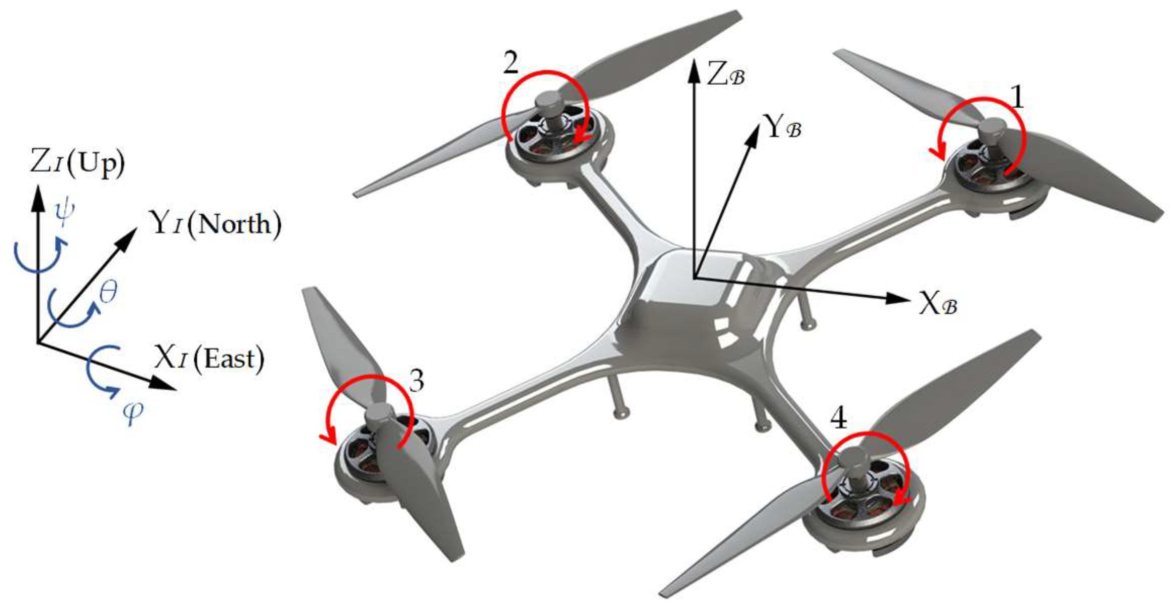
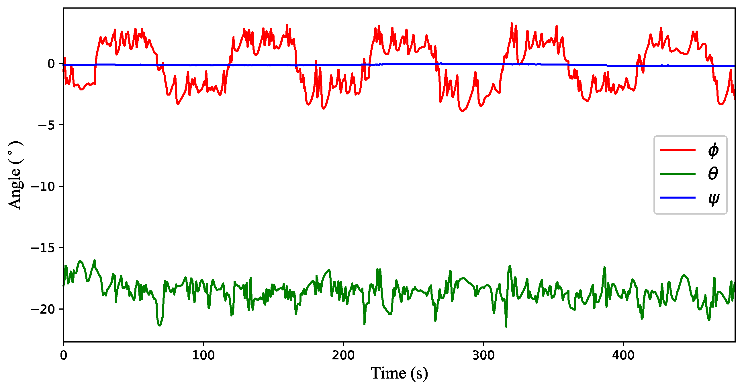
3.1. Dynamic Model of the Rotorcraft
- (1)
- the thrust acceleration , which is the key to calculate ;
- (2)
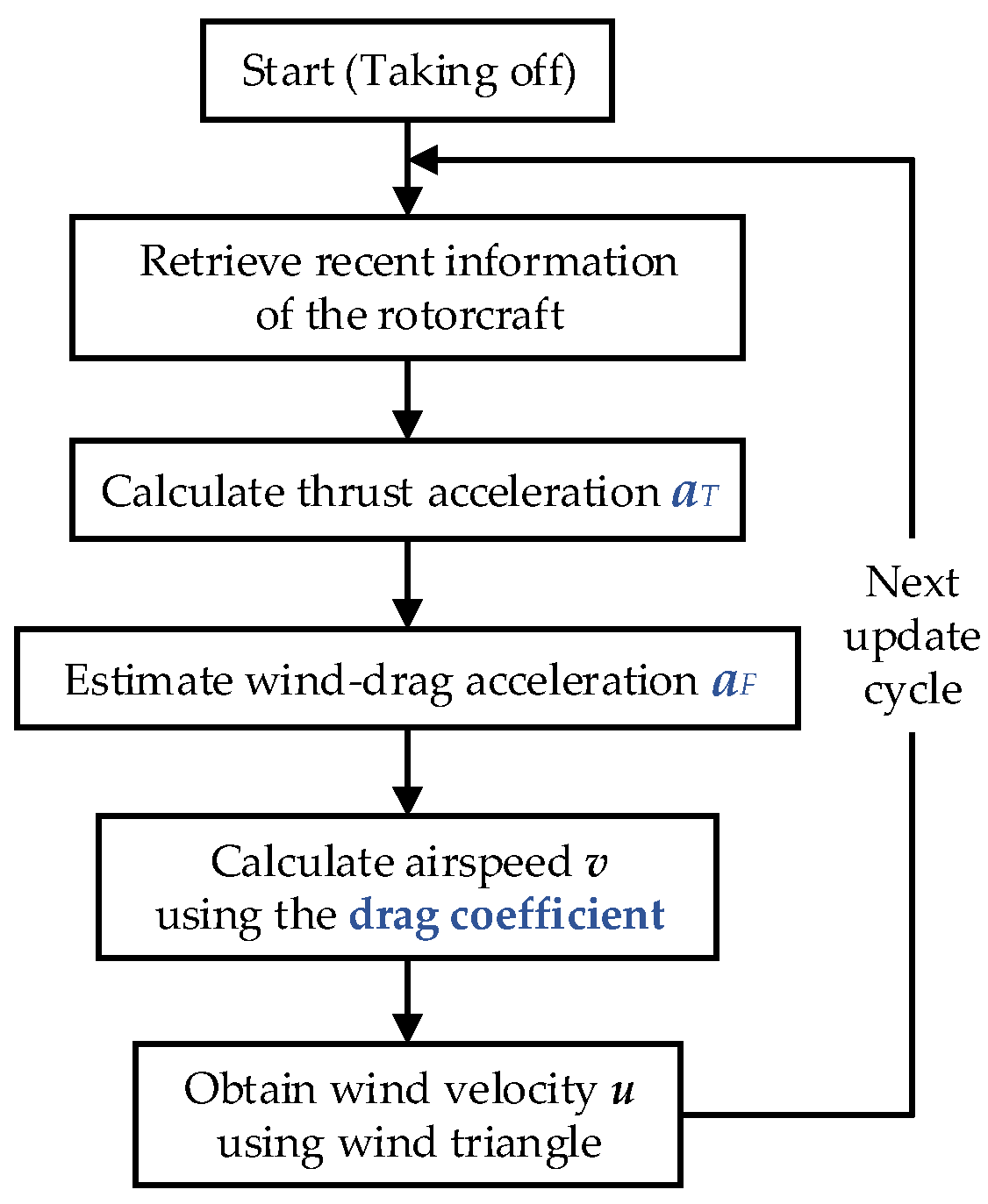
- the wind-drag acceleration . The noise caused by rotorcraft’s accelerometer (for measuring ) and dynamic changes of motors’ supplied voltages (for calculating ) will deteriorate the computed result of by Equation (8) using instantaneous measurements of and . Compared to direct calculation by Equation (8), calculating by a more efficient method is a crucial step;
- (3)
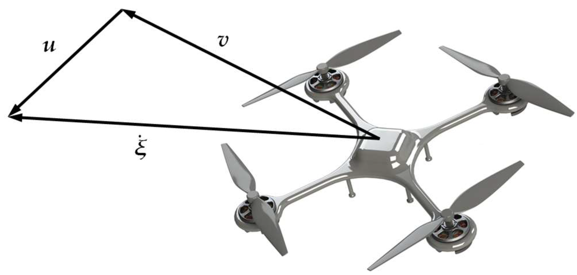
- the drag coefficient C, which is an important parameter to obtain v.
3.2. Calculation of the Thrust Acceleration
3.3. Estimation of the Wind-Drag Acceleration
3.4. Calculation of the Drag Coefficient
| Algorithm 1: Computational procedure of the wind estimation method | ||
| Input: η = ()T, , , , , cx, cy, cz, , tend | ||
| Output: u | ||
| 1: | % Initialize the state vector of the ESO | |
| 2: | whilet < tend do | |
| 3: | update η(t),, U(t) | |
| 4: | calculate and using (1) and (2) | |
| 5: | calculate using (18) | |
| 6: | ||
| 7: | % Update | |
| 8: | % Update | |
| 9: | % Update | |
| 10: | ||
| 11: | % Calculate the airspeed of the rotorcraft | |
| 12: | % Calculate the wind velocity | |
| 13: | end while | |
4. Simulations and Results
4.1. Simulation Environment
4.1.1. Model of the Quadrotor
4.1.2. Model of Environmental Wind
4.2. Simulation Setup
- (1)
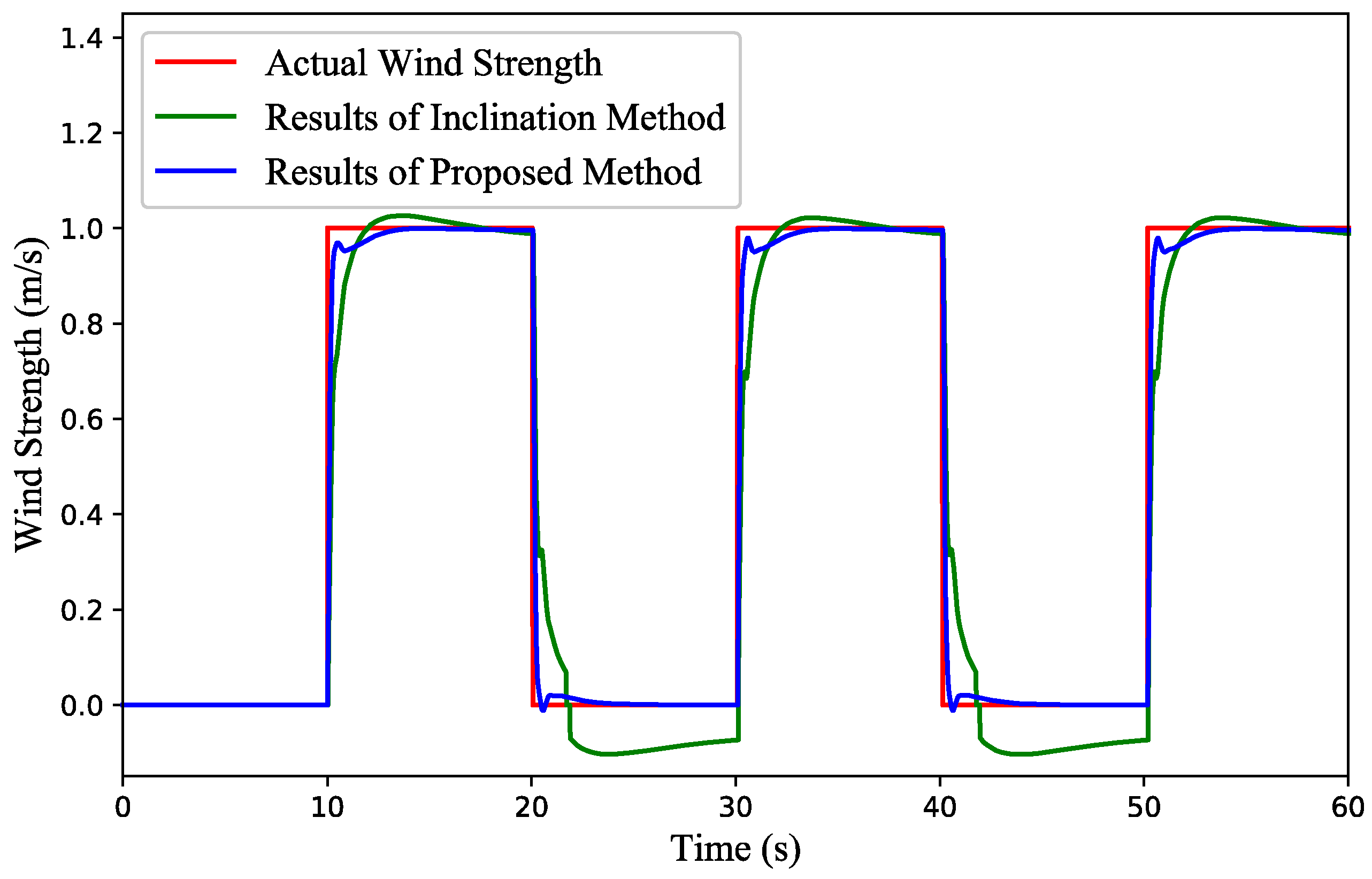
- Test 1: Wind gust estimation with a quadrotor in hovering conditions. The gust wind is simulated with a square wave signal of a 20 s period, and the wind strength is (1, 0, 0) m/s, i.e., the wind blows towards the east. The quadrotor is in hovering condition. The frequencies of the actual and the estimated wind strength/direction signals are set at 50 Hz.
- (2)
- Test 2: Time-varying wind estimation with a quadrotor in hovering conditions. The constant component of the wind strength is set to (2, 0, 0) m/s and the parameter settings of the fluctuating component is presented in Table 2. The quadrotor is in hovering condition.
- (3)
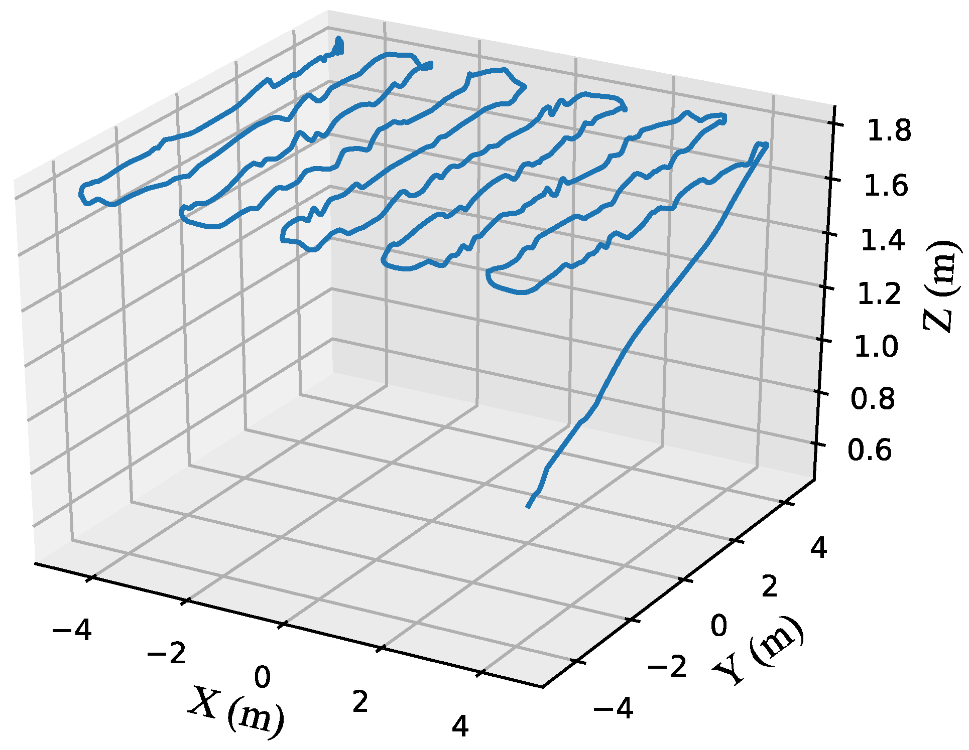
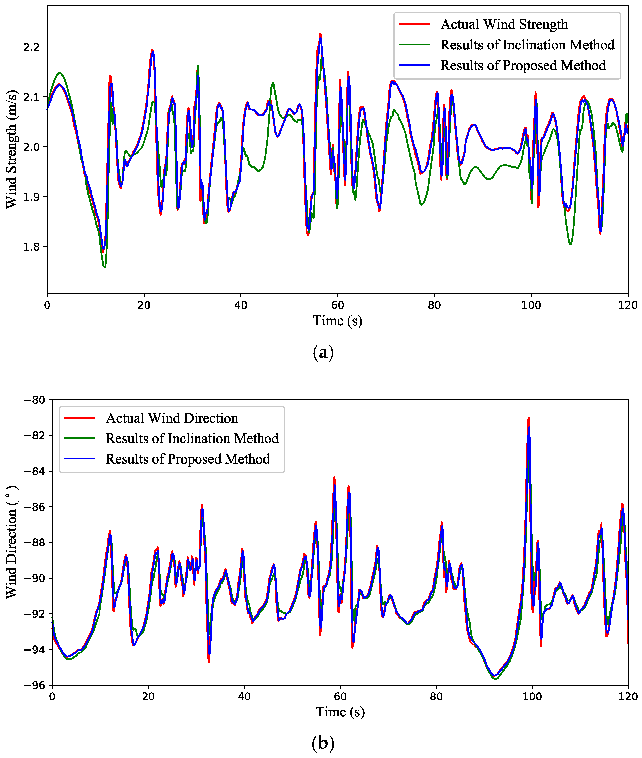
- Test 3: Time-varying wind estimation with a quadrotor in flight conditions. The time-varying wind field is set as that in Test 2. The quadrotor flies in the desired trajectory, and the real flight path is shown in Figure 6.
4.3. Simulation Results
5. Experiments and Results
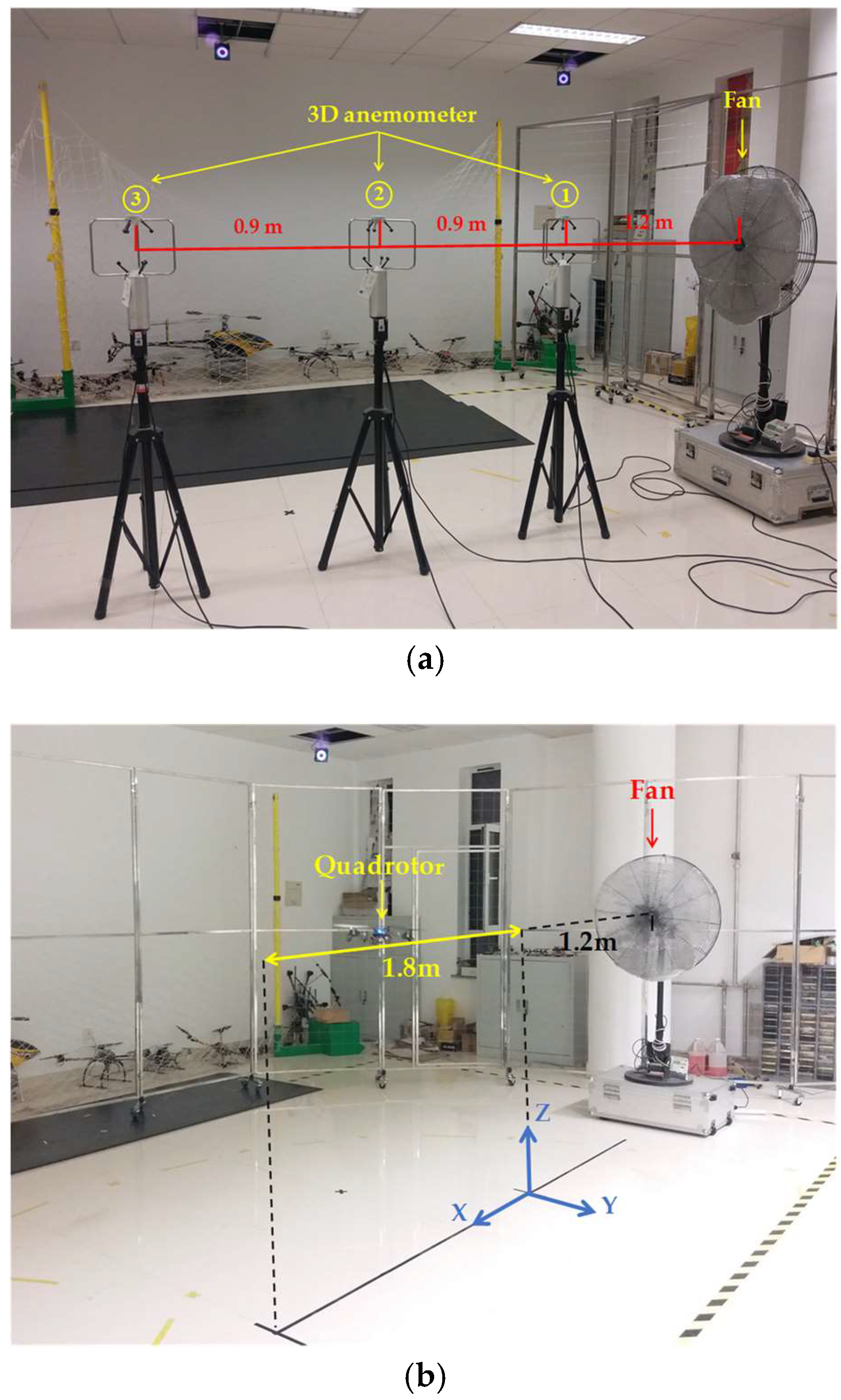
5.1. Experimental Setup
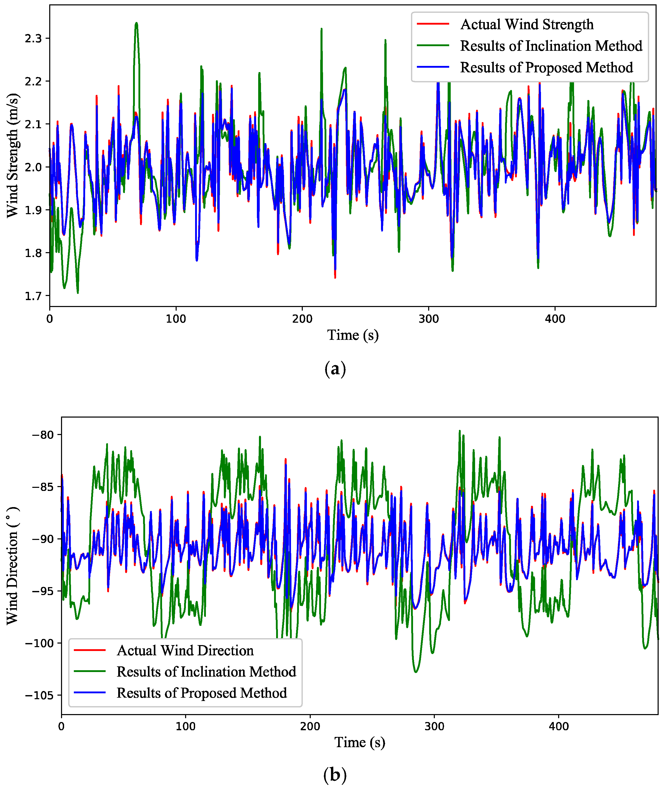
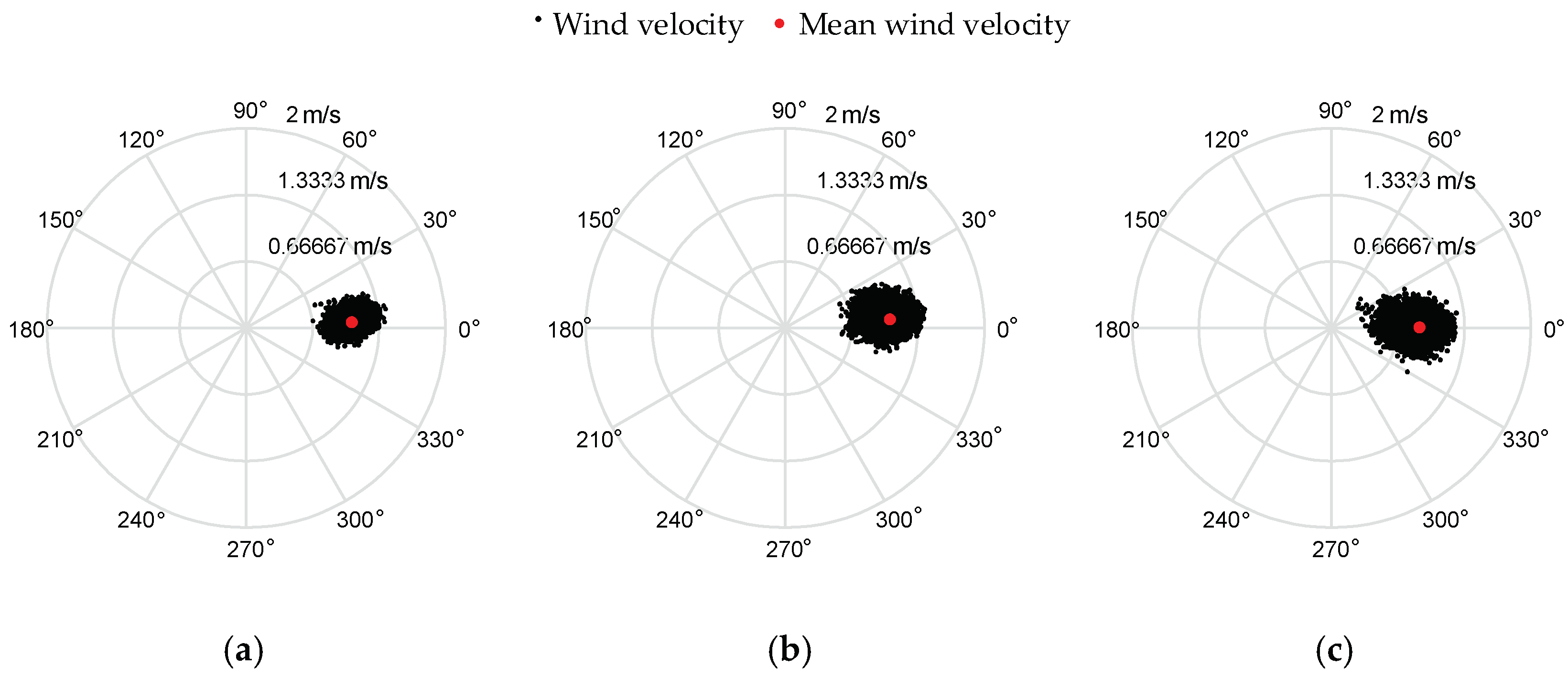
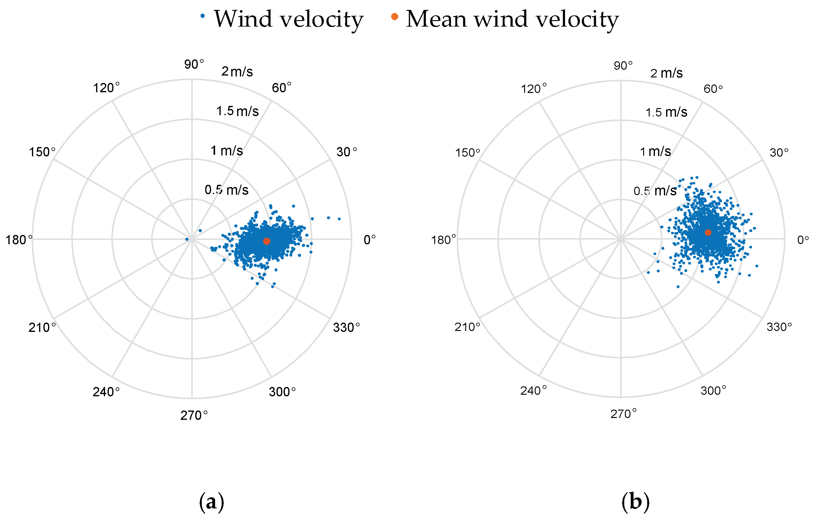
5.2. Experimental Results
6. Conclusions
Author Contributions
Funding
Acknowledgments
Conflicts of Interest
References
- Marino, M.; Fisher, A.; Clothier, R.; Watkins, S.; Prudden, S.; Leung, C.S. An evaluation of multi-rotor unmanned aircraft as flying wind sensors. Int. J. Micro Air Veh. 2015, 7, 285–300. [Google Scholar] [CrossRef]
- Neumann, P.P.; Asadi, S.; Lilienthal, A.J.; Bartholmai, M. Autonomous gas-sensitive microdrone: Wind vector estimation and gas distribution mapping. IEEE Robot. Autom. Mag. 2012, 9, 50–61. [Google Scholar] [CrossRef]
- Neumann, P.P.; Bennetts, V.H.; Lilienthal, A.J.; Bartholmai, M.; Schiller, J.H. Gas source localization with a micro-drone using bio-inspired and particle filter-based algorithms. Adv. Robot. 2013, 27, 725–738. [Google Scholar] [CrossRef]
- Pyk, P.; Badia, S.B.I.; Bernardet, U.; Knüsel, P.; Carlsson, M.; Gu, J.; Chanie, E.; Hansson, B.S.; Pearce, T.C.; Verschure, P.F. An artificial moth: Chemical source localization using a robot based neuronal model of moth optomotor anemotactic search. Auton. Robots 2006, 20, 197–213. [Google Scholar] [CrossRef]
- Ishida, H.; Nakayama, G.; Nakamoto, T.; Moriizumi, T. Controlling a gas/odor plume-tracking robot based on transient responses of gas sensors. IEEE Sens. J. 2005, 5, 537–545. [Google Scholar] [CrossRef]
- Kowadlo, G.; Russell, R.A. Improving the robustness of naïve physics airflow mapping, using bayesian reasoning on a multiple hypothesis tree. Robot. Auton. Syst. 2009, 57, 723–737. [Google Scholar] [CrossRef]
- Zarzhitsky, D.V.; Spears, D.F.; Thayer, D.R. Experimental studies of swarm robotic chemical plume tracing using computational fluid dynamics simulations. Int. J. Intell. Comput. Cybern. 2010, 3, 631–671. [Google Scholar] [CrossRef]
- Pang, S.; Farrell, J.A. Chemical plume source localization. IEEE Trans. Syst. Man Cybern. B 2006, 36, 1068–1080. [Google Scholar] [CrossRef]
- Li, J.-G.; Meng, Q.-H.; Wang, Y.; Zeng, M. Odor source localization using a mobile robot in outdoor airflow environments with a particle filter algorithm. Auton. Robots 2011, 30, 281–292. [Google Scholar] [CrossRef]
- Marques, L.; Nunes, U.; Almeida, A.T. Particle swarm-based olfactory guided search. Auton. Robots 2006, 20, 277–287. [Google Scholar] [CrossRef]
- Bruschi, P.; Piotto, M.; Dell’Agnello, F.; Ware, J.; Roy, N. Wind speed and direction detection by means of solid-state anemometers embedded on small quadcopters. Procedia Eng. 2016, 168, 802–805. [Google Scholar] [CrossRef]
- Arain, B.; Kendoul, F. Real-time wind speed estimation and compensation for improved flight. IEEE Trans. Aerosp. Electron. Syst. 2014, 50, 1599–1606. [Google Scholar] [CrossRef]
- Waslander, S.; Wang, C. Wind disturbance estimation and rejection for quadrotor position control. In Proceedings of the AIAA Infotech@Aerospace Conference, Washington, DC, USA, 6–7 April 2009. [Google Scholar]
- Gonzalez-Rocha, J.; Woolsey, C.A.; Sultan, C.; Wekker, S.D.; Rose, N. Measuring atmospheric winds from quadrotor motion. In Proceedings of the AIAA Atmospheric Flight Mechanics Conference, Grapevine, TX, USA, 9–13 January 2017. [Google Scholar]
- Müller, K.; Crocoll, P.; Trommer, G.F. Wind estimation for a quadrotor helicopter in a model-aided navigation system. In Proceedings of the 22nd Saint Petersburg International Conference on Integrated Navigation Systems, Saint Petersburg, Russia, 25–27 May 2019; pp. 45–48. [Google Scholar]
- Müller, K.; Crocoll, P.; Trommer, G.F. Model-aided navigation with wind estimation for robust quadrotor navigation. In Proceedings of the 2016 International Technical Meeting of the Institute of Navigation, Monterey, CA, USA, 25–28 January 2016; pp. 689–696. [Google Scholar]
- Sikkel, L.N.C.; Croon, G.D.; Wagter, C.D.; Chu, Q.P. A novel online model-based wind estimation approach for quadrotor micro air vehicles using low cost MEMS IMUs. In Proceedings of the IEEE/RSJ Intelligent Robots and Systems (IROS), Daejeon, Korea, 9–14 October 2016; pp. 2141–2146. [Google Scholar] [CrossRef]
- Schiano, F.; Alonso-Mora, J.; Rudin, K.; Beardsley, P.; Siegwart, R.; Sicilianok, B. Towards estimation and correction of wind effects on a quadrotor UAV. In Proceedings of the International Micro Air Vehicle Conference and Competition (IMAV), Delft, The Netherlands, 12–15 August 2014; pp. 134–141. [Google Scholar] [CrossRef]
- Neumann, P.P.; Bartholmai, M. Real-time wind estimation on a micro unmanned aerial vehicle using its inertial measurement unit. Sens. Actuators A Phys. 2015, 235, 300–310. [Google Scholar] [CrossRef]
- Palomaki, R.T.; Rose, N.T.; Bossche, M.V.D.; Sherman, T.J.; Wekker, S.F.J.D. Wind estimation in the lower atmosphere using multirotor aircraft. J. Atmos. Ocean. Technol. 2017, 34, 1183–1191. [Google Scholar] [CrossRef]
- Eu, K.S.; Wei, Z.C.; Yap, K.M. Wind direction and speed estimation for quadrotor based gas tracking robot. In Mobile and Wireless Technologies 2017; Springer: Singapore, 2017; pp. 645–652. [Google Scholar]
- Song, Y.; Luo, B.; Meng, Q.-H. A rotor-aerodynamics-based wind estimation method using a quadrotor. Meas. Sci. Technol. 2018, 29, 025801. [Google Scholar] [CrossRef]
- Hüllmann, D.; Paul, N.; Neumann, P.P. Motor speed transfer function for wind vector estimation on multirotor aircraft. In Proceedings of the 34th Danubia-Adria Symposium on Advances in Experimental Mechanics, Trieste, Italy, 19–22 September 2017. [Google Scholar]
- Han, J.-Q. From PID to active disturbance rejection control. IEEE Trans. Ind. Electron. 2009, 56, 900–906. [Google Scholar] [CrossRef]
- Yang, H.-J.; Cheng, L.; Xia, Y.-Q.; Yuan, Y. Active disturbance rejection attitude control for a dual closed-loop quadrotor under gust wind. IEEE Trans. Control Syst. Technol. 2018, 26, 1400–1405. [Google Scholar] [CrossRef]
- Han, J.-Q. A class of extended state observers for uncertain systems. Control Decis. 1995, 10, 85–88. (In Chinese) [Google Scholar]
- Guo, B.-Z.; Zhao, Z.-L. On the convergence of an extended state observer for nonlinear systems with uncertainty. Syst. Control Lett. 2011, 60, 420–430. [Google Scholar] [CrossRef]
- Bouadi, H.; Tadjine, M. Nonlinear observer design and sliding mode control of four rotors helicopter. Int. J. Mech. Aerosp. Ind. Mechatron. Manuf. Eng. 2007, 1, 354–359. [Google Scholar]
- Luukkonen, T. Modelling and Control of Quadcopter; Independent Research Project in Applied Mathematics: Espoo, Finland, 2011. [Google Scholar]
- Xue, W.-C.; Bai, W.-Y.; Yang, S.; Song, K.; Huang, Y.; Xie, H. ADRC with adaptive extended state observer and its application to air–fuel ratio control in gasoline engines. IEEE Trans. Ind. Electron. 2015, 62, 5847–5857. [Google Scholar] [CrossRef]
- Rida, M.M.; Choukchou, B.A.; Cherki, B. Extended state observer based control for coaxial-rotor UAV. Isa Trans. 2016, 61, 1–14. [Google Scholar] [CrossRef] [PubMed]
- Gao, Z.-Q. Scaling and parameterization based controller tuning. In Proceedings of the 2003 American Control Conference, Denver, CO, USA, 4–6 June 2003; pp. 4989–4996. [Google Scholar] [CrossRef]
- Luo, B.; Meng, Q.-H.; Wang, J.-Y.; Ma, S.-G. Simulate the aerodynamic olfactory effects of gas-sensitive UAVs: A numerical model and its parallel implementation. Adv. Eng. Softw. 2016, 102, 123–133. [Google Scholar] [CrossRef]
- Farrell, J.A.; Murlis, J.; Long, X.; Li, W.; Cardé, R.T. Filament-based atmospheric dispersion model to achieve short time-scale structure of odor plumes. Environ. Fluid Mech. 2002, 2, 143–169. [Google Scholar] [CrossRef]


| Parameter | Value |
|---|---|
| m (kg) | 0.122 |
| L (m) | 0.11 |
| J | diag (0.0002632, 0.0002745, 0.00091175) |
| k | 0.0000542 |
| b | 0.000011 |
| Parameter | Value |
|---|---|
| 0.3, 0.3, 0.3 | |
| 0.05, 0.05, 0.05 | |
| G | 10 |
| Simulation Scenario | RMSE of Wind Strength (m/s) | RMSE of Wind Direction (°) | |
|---|---|---|---|
| Test 1 | Inclination method | 0.1287 | / |
| Proposed method | 0.0796 | / | |
| Test 2 | Inclination method | 0.0481 | 0.6889 |
| Proposed method | 0.0154 | 0.3723 | |
| Test 3 | Inclination method | 0.0708 | 5.4621 |
| Proposed method | 0.0156 | 0.4558 | |
| Statistical Indicators | Anemometer 1 | Anemometer 2 | Anemometer 3 |
|---|---|---|---|
| Mean value of wind strength (m/s) | 1.0616 | 1.0551 | 0.8812 |
| Mean value of wind direction (°) | 3.1240 | 4.6850 | 0.5207 |
| Standard deviation of wind strength (m/s) | 0.0941 | 0.1088 | 0.1208 |
| Standard deviation of wind direction (°) | 3.1985 | 4.3714 | 5.3590 |
| Statistical Indicators | Hover Test | Flight Test 1 | Flight Test 2 | Flight Test 3 |
|---|---|---|---|---|
| Mean value of wind strength (m/s) | 0.9384 | 1.0681 | 1.0773 | 1.0983 |
| Mean value of wind direction (°) | −1.7664 | 4.2946 | 4.4181 | 0.8479 |
| Standard deviation of wind strength (m/s) | 0.1751 | 0.1710 | 0.1910 | 0.2009 |
| Standard deviation of wind direction (°) | 9.3774 | 11.2742 | 10.6558 | 10.6584 |
© 2018 by the authors. Licensee MDPI, Basel, Switzerland. This article is an open access article distributed under the terms and conditions of the Creative Commons Attribution (CC BY) license (http://creativecommons.org/licenses/by/4.0/).
Share and Cite
Wang, J.-Y.; Luo, B.; Zeng, M.; Meng, Q.-H. A Wind Estimation Method with an Unmanned Rotorcraft for Environmental Monitoring Tasks. Sensors 2018, 18, 4504. https://doi.org/10.3390/s18124504
Wang J-Y, Luo B, Zeng M, Meng Q-H. A Wind Estimation Method with an Unmanned Rotorcraft for Environmental Monitoring Tasks. Sensors. 2018; 18(12):4504. https://doi.org/10.3390/s18124504
Chicago/Turabian StyleWang, Jia-Ying, Bing Luo, Ming Zeng, and Qing-Hao Meng. 2018. "A Wind Estimation Method with an Unmanned Rotorcraft for Environmental Monitoring Tasks" Sensors 18, no. 12: 4504. https://doi.org/10.3390/s18124504
APA StyleWang, J.-Y., Luo, B., Zeng, M., & Meng, Q.-H. (2018). A Wind Estimation Method with an Unmanned Rotorcraft for Environmental Monitoring Tasks. Sensors, 18(12), 4504. https://doi.org/10.3390/s18124504