Answering the Min-Cost Quality-Aware Query on Multi-Sources in Sensor-Cloud Systems †


Abstract
1. Introduction
- A general definition of MQQ answering problem is provided.
- The data quality measurement of quality-aware query on multi-sources is defined based on relative data quality constraints. Two methods for solving the min-cost quality-aware query answering problem are proposed.
- If the users do not have enough knowledge of the data, it is often difficult for them to set the reasonable quality threshold. To deal with this problem, a method is proposed to automatically help the users to find a proper quality threshold.
- The experiments on real-life data are conducted, which verifies the efficiency and effectiveness of the provided solutions.
2. Related Work
3. A General Definition of MQQ Answering Problem
3.1. Preliminaries
3.2. Definition of MQQ Answering Problem
- For each , such that is the observation of o, that is, contains the observations of all queried objects,
- can satisfy the quality lower bound ,
- returned by such that satisfies condition (1) and (2), and .
4. Measuring Data Quality Based on Quality Constraints
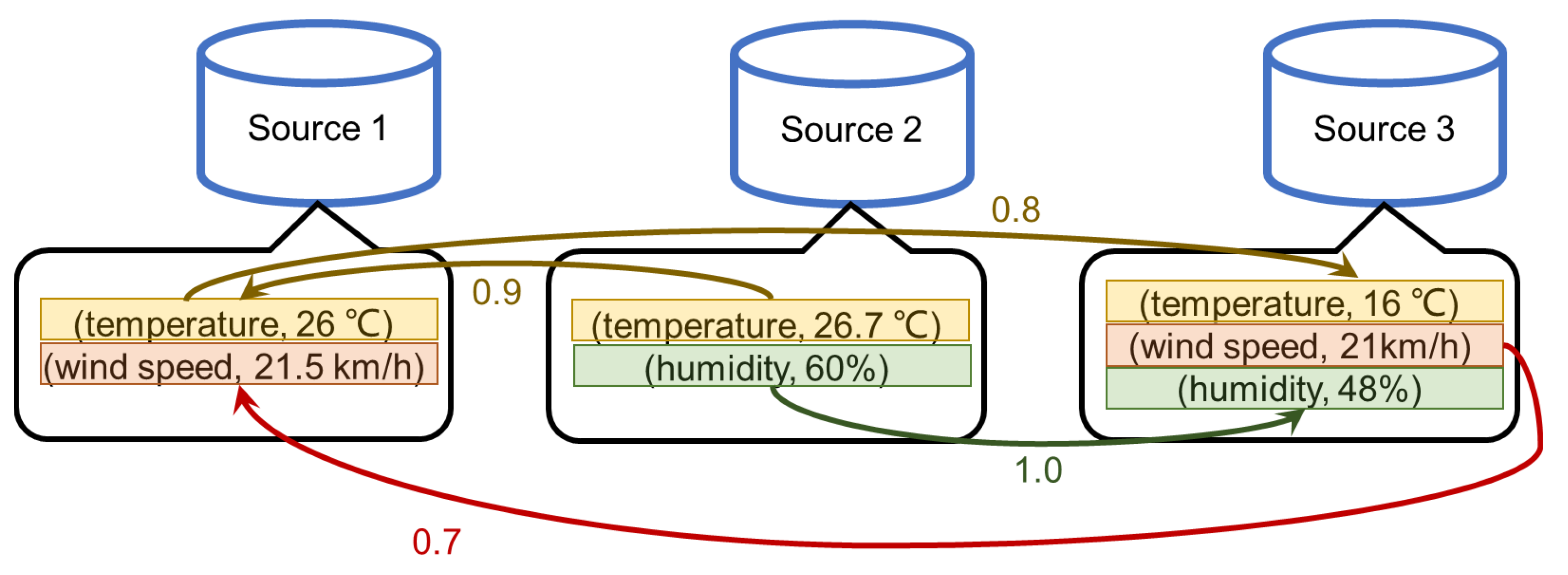
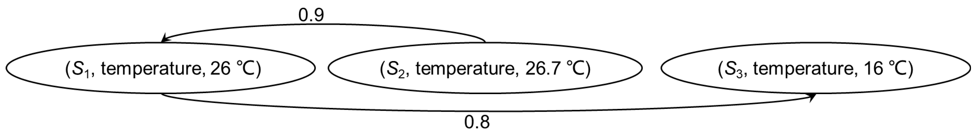
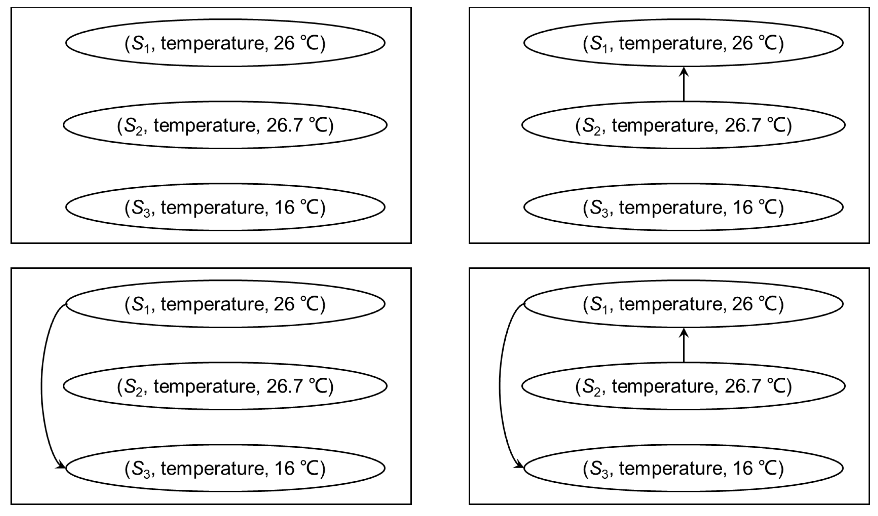
4.1. Quality Graph
- 1.
- Each node corresponds to an observation in .
- 2.
- For each pair , if , there exists an arc from ϕ to in A, the weight of the arc is .
4.2. Data Quality Score
5. Methods for Solving MQQ Answering Problem
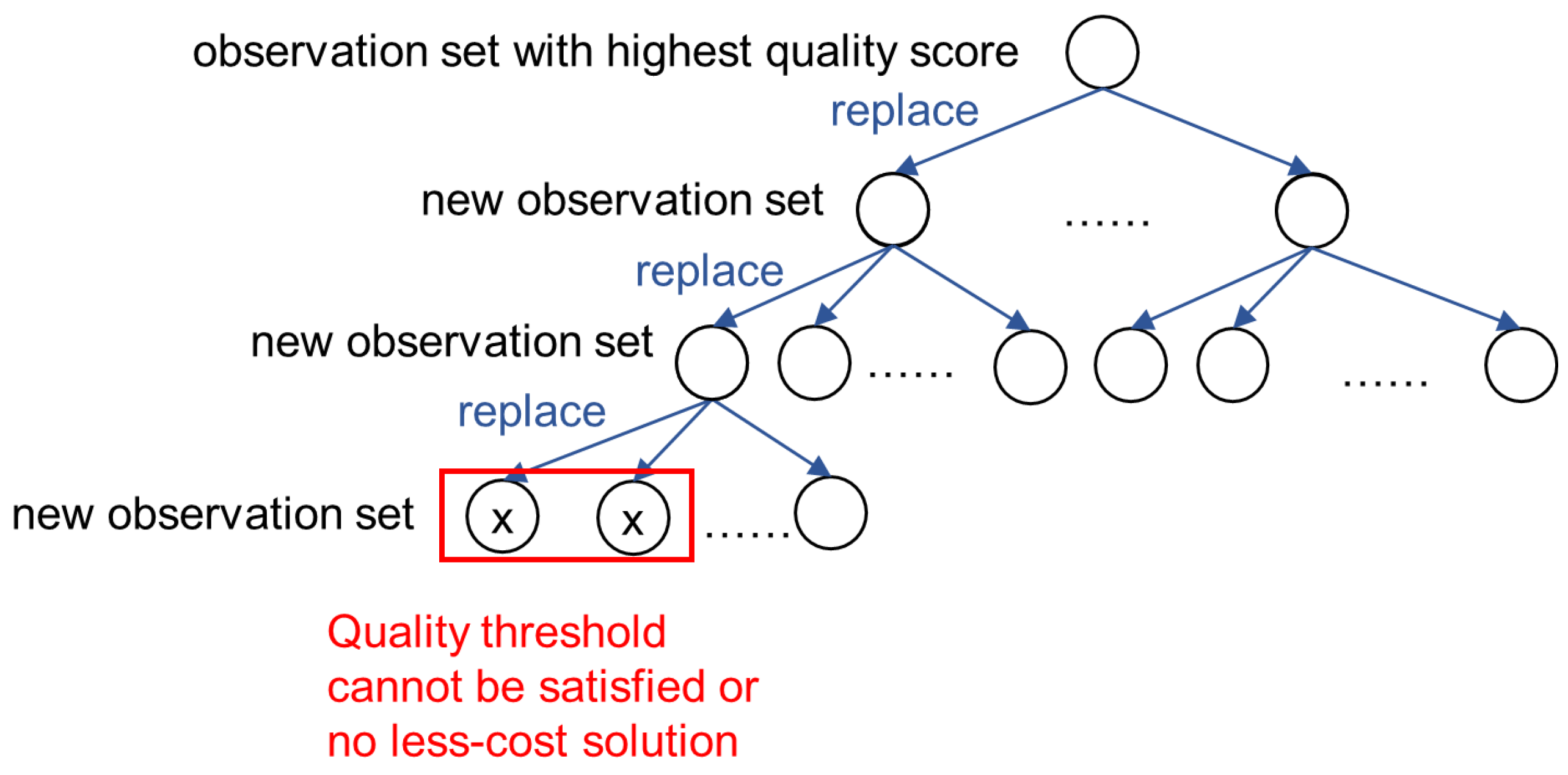
5.1. The Search and Prune Method
5.2. Approximate Search
5.3. Discussions
- For the two search strategies, it is very important to efficiently get the next data source to do the replacement. To this end, ordered lists can be maintained, and the ith ordered list stores the high-to-low ordering of the sources that can provide object . A element of the ordered list is a quad of the form , where is a pointer to the next quad in the ordered list. Thus, during the search, we can use to calculate the quality score of the current search tree node, and use to get the next data source that can be used to do the replacement in constant time.
- Different branches of the search tree may have the same node. In implementation, we can first check to see if the current node already has a duplicate that has been processed. The node is discarded if the answer is yes. This operation can avoid repeating process and can save a lot of time.
6. A Method for Selecting the Quality Threshold
6.1. Determining the Reasonability of a Threshold
- The quality threshold is set too high such that no observation set can satisfy the threshold.
- The quality threshold is set too low, which is likely to cause large search space, and to lead to unendurable query latency.
6.1.1. Deal with High Threshold
6.1.2. Deal with Low Threshold
6.2. Finding a Reasonable Threshold
- If the threshold is considered to be too high, we only need to return the quality score of the root node of the search tree and tell the user that there is no query result higher than this score.
- If the threshold is considered to be too low, we need to return a set of candidates to guide the user in adjusting the threshold. As stated in Theorem 1, when the search tree is expanded to the lower layer, is not increased (i.e., the value of only decreases or keeps unchanged). Therefore, in the estimation process, the layer where changes can be recorded and converted into a query latency. That is, we ignore those layers whose is unchanged and record the layers whose decreases. The historical data can be used to learn the possible query latency regarding the number of layers. The recorded can be given to the user as a candidate set to help the user to adjust the threshold setting.
7. Experimental Results
7.1. Performance of the Search Methods
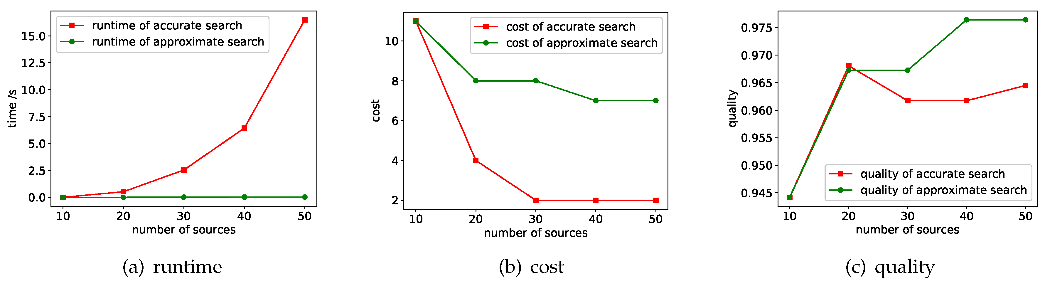
7.1.1. Varying
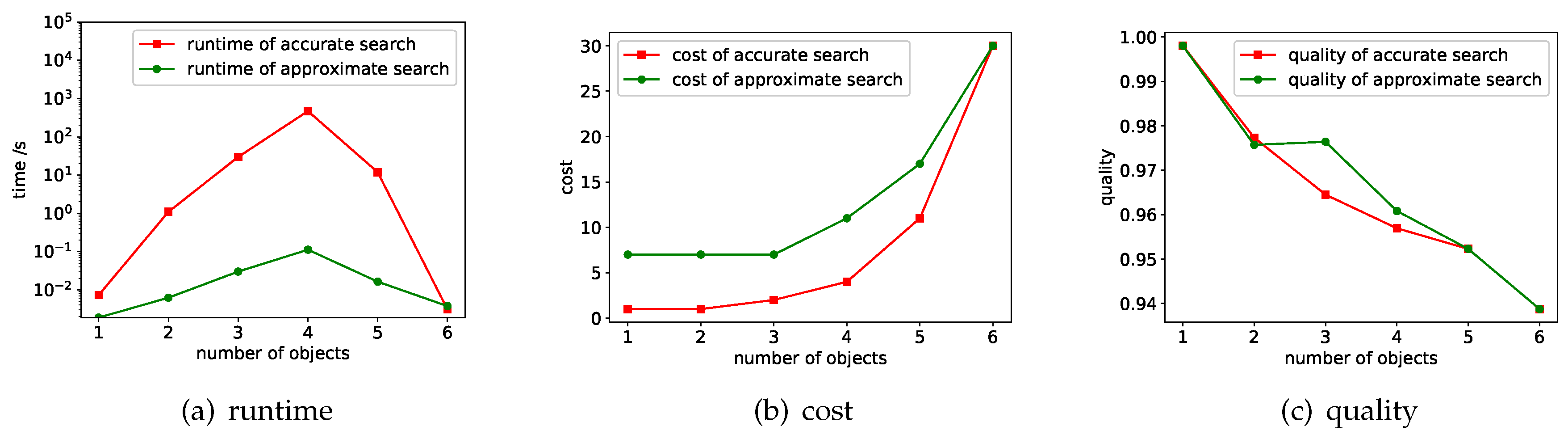
7.1.2. Varying
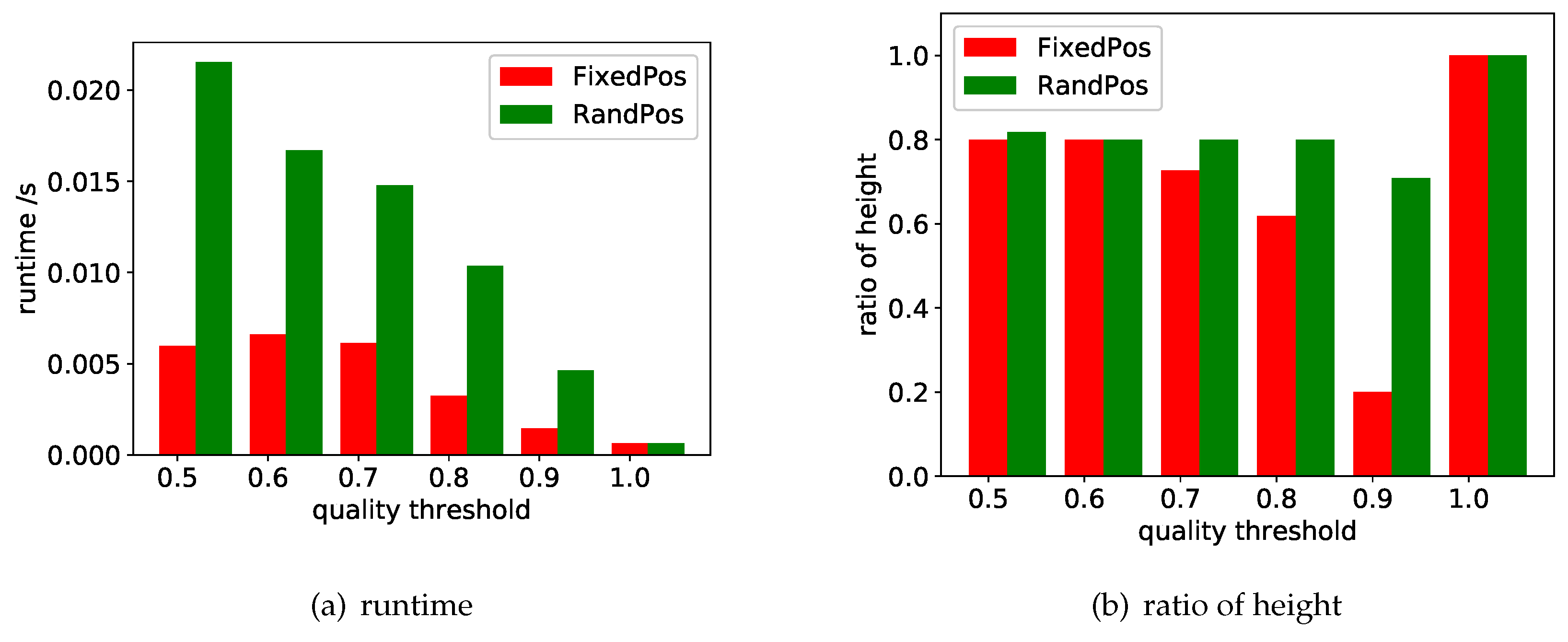
7.2. Evaluation of Search Space Size Estimation
8. Conclusions and Future Work
Author Contributions
Funding
Conflicts of Interest
References
- Rahm, E.; Do, H.H. Data cleaning: Problems and current approaches. IEEE Data Eng. Bull. 2000, 24, 3–13. [Google Scholar]
- Lazaridis, I.; Han, Q.; Yu, X.; Mehrotra, S.; Venkatasubramanian, N.; Kalashnikov, D.V.; Yang, W. Quasar: Quality aware sensing architecture. ACM SIGMOD Rec. 2004, 33, 26–31. [Google Scholar] [CrossRef]
- Alamri, A.; Ansari, W.S.; Hassan, M.M.; Hossain, M.S.; Alelaiwi, A.; Hossain, M.A. A survey on sensor-cloud: Architecture, applications, and approaches. Int. J. Distrib. Sens. Netw. 2013, 9, 917923. [Google Scholar] [CrossRef]
- Wang, T.; Zhang, G.; Liu, A.; Bhuiyan, M.Z.A.; Jin, Q. A Secure IoT Service Architecture with an Efficient Balance Dynamics Based on Cloud and Edge Computing. IEEE Internet Things J. 2018. [Google Scholar] [CrossRef]
- Wang, T.; Zhou, J.; Liu, A.; Bhuiyan, M.Z.A.; Wang, G.; Jia, W. Fog-based Computing and Storage Offloading for Data Synchronization in IoT. IEEE Internet Things J. 2018. [Google Scholar] [CrossRef]
- Wang, T.; Zhang, G.; Bhuiyan, M.Z.A.; Liu, A.; Jia, W.; Xie, M. A novel trust mechanism based on Fog Computing in Sensor–Cloud System. Future Gener. Comput. Syst. 2018. [Google Scholar] [CrossRef]
- Li, M.; Jiang, Y.; Sun, Y.; Tian, Z. Answering the Min-cost Quality-aware Query on Multi-sources in Sensor-Cloud Systems. In Proceedings of the The Fourth International Symposium on Sensor-Cloud Systems (SCS 2018), Melbourne, Australia, 11–13 December 2018. [Google Scholar]
- Fan, W.; Geerts, F. Foundations of data quality management. Synth. Lect. Data Manag. 2012, 4, 1–217. [Google Scholar] [CrossRef]
- Rammelaere, J.; Geerts, F.; Goethals, B. Cleaning Data with Forbidden Itemsets. In Proceedings of the 2017 IEEE 33rd International Conference on Data Engineering (ICDE), San Diego, CA, USA, 19–22 April 2017; pp. 897–908. [Google Scholar]
- Fan, W.; Geerts, F.; Jia, X.; Kementsietsidis, A. Conditional Functional Dependencies for Capturing Data Inconsistencies. ACM Trans. Database Syst. 2008. [Google Scholar] [CrossRef]
- Fan, W.; Geerts, F.; Wijsen, J. Determining the currency of data. ACM Trans. Database Syst. 2012, 37, 25. [Google Scholar] [CrossRef]
- Chu, X.; Ilyas, I.F.; Papotti, P. Holistic data cleaning: Putting violations into context. In Proceedings of the IEEE 29th International Conference on Data Engineering (ICDE), Brisbane, Australia, 8–12 April 2013; pp. 458–469. [Google Scholar]
- Rekatsinas, T.; Joglekar, M.; Garcia-Molina, H.; Parameswaran, A.; Ré, C. SLiMFast: Guaranteed results for data fusion and source reliability. In Proceedings of the 2017 ACM International Conference on Management of Data, Chicago, IL, USA, 14–19 May 2017; ACM: New York, NY, USA, 2017; pp. 1399–1414. [Google Scholar]
- Cao, Y.; Fan, W.; Yu, W. Determining the relative accuracy of attributes. In Proceedings of the 2013 ACM SIGMOD International Conference on Management of Data, New York, NY, USA, 22–27 June 2013. [Google Scholar]
- Fan, W.; Geerts, F. Relative information completeness. ACM Trans. Database Syst. 2010, 35, 27. [Google Scholar] [CrossRef]
- Li, M.; Li, J.; Cheng, S.; Sun, Y. Uncertain Rule Based Method for Determining Data Currency. IEICE Trans. Inf. Syst. 2018, 101, 2447–2457. [Google Scholar] [CrossRef]
- Li, M.; Li, J. A minimized-rule based approach for improving data currency. J. Comb. Optim. 2016, 32, 812–841. [Google Scholar] [CrossRef]
- Dong, X.L.; Gabrilovich, E.; Murphy, K.; Dang, V.; Horn, W.; Lugaresi, C.; Sun, S.; Zhang, W. Knowledge-based trust: Estimating the trustworthiness of web sources. Proc. VLDB Endow. 2015, 8, 938–949. [Google Scholar] [CrossRef]
- Dong, X.L.; Berti-Equille, L.; Srivastava, D. Integrating conflicting data: The role of source dependence. Proc. VLDB Endow. 2009, 2, 550–561. [Google Scholar] [CrossRef]
- Lin, X.; Chen, L. Domain-aware multi-truth discovery from conflicting sources. Proc. VLDB Endow. 2018, 11, 635–647. [Google Scholar]
- Dong, X.L.; Berti-Equille, L.; Srivastava, D. Truth discovery and copying detection in a dynamic world. Proc. VLDB Endow. 2009, 2, 562–573. [Google Scholar] [CrossRef]
- Dong, X.L.; Berti-Equille, L.; Hu, Y.; Srivastava, D. Global detection of complex copying relationships between sources. Proc. VLDB Endow. 2010, 3, 1358–1369. [Google Scholar] [CrossRef]
- Madria, S.; Kumar, V.; Dalvi, R. Sensor cloud: A cloud of virtual sensors. IEEE Softw. 2014, 31, 70–77. [Google Scholar] [CrossRef]
- Santos, I.L.; Pirmez, L.; Delicato, F.C.; Khan, S.U.; Zomaya, A.Y. Olympus: The cloud of sensors. IEEE Cloud Comput. 2015, 2, 48–56. [Google Scholar] [CrossRef]
- Fazio, M.; Puliafito, A. Cloud4sens: A cloud-based architecture for sensor controlling and monitoring. IEEE Commun. Mag. 2015, 53, 41–47. [Google Scholar] [CrossRef]
- Lyu, Y.; Yan, F.; Chen, Y.; Wang, D.; Shi, Y.; Agoulmine, N. High-performance scheduling model for multisensor gateway of cloud sensor system-based smart-living. Inf. Fusion 2015, 21, 42–56. [Google Scholar] [CrossRef]
- Abdelwahab, S.; Hamdaoui, B.; Guizani, M.; Znati, T. Cloud of things for sensing-as-a-service: Architecture, algorithms, and use case. IEEE Internet Things J. 2016, 3, 1099–1112. [Google Scholar] [CrossRef]
- Zhu, C.; Leung, V.C.; Wang, K.; Yang, L.T.; Zhang, Y. Multi-method data delivery for green sensor-cloud. IEEE Commun. Mag. 2017, 55, 176–182. [Google Scholar] [CrossRef]
- Dinh, T.; Kim, Y.; Lee, H. A Location-Based Interactive Model of Internet of Things and Cloud (IoT-Cloud) for Mobile Cloud Computing Applications. Sensors 2017, 17, 489. [Google Scholar] [CrossRef]
- Wang, Y.; Tian, Z.; Zhang, H.; Su, S.; Shi, W. A Privacy Preserving Scheme for Nearest Neighbor Query. Sensors 2018, 18, 2440. [Google Scholar] [CrossRef]
- Tian, Z.; Cui, Y.; An, L.; Su, S.; Yin, X.; Yin, L.; Cui, X. A Real-Time Correlation of Host-Level Events in Cyber Range Service for Smart Campus. IEEE Access 2018, 6, 35355–35364. [Google Scholar] [CrossRef]
- Tan, Q.; Gao, Y.; Shi, J.; Wang, X.; Fang, B.; Tian, Z.H. Towards a Comprehensive Insight into the Eclipse Attacks of Tor Hidden Services. IEEE Internet Things J. 2018. [Google Scholar] [CrossRef]
- Yu, X.; Tian, Z.; Qiu, J.; Jiang, F. A Data Leakage Prevention Method Based on the Reduction of Confidential and Context Terms for Smart Mobile Devices. Wirel. Commun. Mob. Comput. 2018, 2018, 11. [Google Scholar] [CrossRef]
- Jiang, F.; Fu, Y.; Gupta, B.B.; Lou, F.; Rho, S.; Meng, F.; Tian, Z. Deep Learning based Multi-channel intelligent attack detection for Data Security. IEEE Trans. Sustain. Comput. 2018. [Google Scholar] [CrossRef]
- Chen, J.; Tian, Z.; Cui, X.; Yin, L.; Wang, X. Trust architecture and reputation evaluation for internet of things. J. Ambient Intell. Humaniz. Comput. 2018, 1–9. [Google Scholar] [CrossRef]
- Zhihong, T.; Wei, J.; Yang, L. A transductive scheme based inference techniques for network forensic analysis. China Commun. 2015, 12, 167–176. [Google Scholar]
- Zhihong, T.; Wei, J.; Yang, L.; Lan, D. A digital evidence fusion method in network forensics systems with Dempster-shafer theory. China Commun. 2014, 11, 91–97. [Google Scholar]
- Lian, X.; Chen, L.; Wang, G. Quality-aware subgraph matching over inconsistent probabilistic graph databases. IEEE Trans. Know. Data Eng. 2016, 28, 1560–1574. [Google Scholar] [CrossRef]
- Yeganeh, N.K.; Sadiq, S.; Sharaf, M.A. A framework for data quality aware query systems. Inf. Syst. 2014, 46, 24–44. [Google Scholar] [CrossRef]
- Wu, H.; Luo, Q.; Li, J.; Labrinidis, A. Quality aware query scheduling in wireless sensor networks. In Proceedings of the Sixth International Workshop on Data Management for Sensor Networks, Lyon, France, 24 August 2009; ACM: New York, NY, USA, 2009; p. 7. [Google Scholar]
- Chu, X.; Ilyas, I.F.; Papotti, P. Discovering denial constraints. Proc. VLDB Endow. 2013, 6, 1498–1509. [Google Scholar] [CrossRef]
- Kruse, S.; Naumann, F. Efficient discovery of approximate dependencies. Proc. VLDB Endow. 2018, 11, 759–772. [Google Scholar] [CrossRef]
- Zou, Z.; Gao, H.; Li, J. Discovering Frequent Subgraphs over Uncertain Graph Databases Under Probabilistic Semantics. In Proceedings of the 16th ACM SIGKDD International Conference on Knowledge Discovery and Data Mining, Washington, DC, USA, 25–28 July 2010; pp. 633–642. [Google Scholar]
- Zou, Z.; Li, J.; Gao, H.; Zhang, S. Frequent Subgraph Pattern Mining on Uncertain Graph Data. In Proceedings of the 18th ACM Conference on Information and Knowledge Management, Hong Kong, China, 2–6 November 2009; pp. 583–592. [Google Scholar]
- Abiteboul, S.; Kanellakis, P.; Grahne, G. On the representation and querying of sets of possible worlds. Theor. Comput. Sci. 1991, 78, 159–187. [Google Scholar] [CrossRef]
- Garey, M.R.; Johnson, D.S. Computers and Intractability. A Guide to the Theory of NP-Completeness; WH Freeman and Co.: San Francisco, CA, USA, 1979. [Google Scholar]


© 2018 by the authors. Licensee MDPI, Basel, Switzerland. This article is an open access article distributed under the terms and conditions of the Creative Commons Attribution (CC BY) license (http://creativecommons.org/licenses/by/4.0/).
Share and Cite
Li, M.; Sun, Y.; Jiang, Y.; Tian, Z. Answering the Min-Cost Quality-Aware Query on Multi-Sources in Sensor-Cloud Systems. Sensors 2018, 18, 4486. https://doi.org/10.3390/s18124486
Li M, Sun Y, Jiang Y, Tian Z. Answering the Min-Cost Quality-Aware Query on Multi-Sources in Sensor-Cloud Systems. Sensors. 2018; 18(12):4486. https://doi.org/10.3390/s18124486
Chicago/Turabian StyleLi, Mohan, Yanbin Sun, Yu Jiang, and Zhihong Tian. 2018. "Answering the Min-Cost Quality-Aware Query on Multi-Sources in Sensor-Cloud Systems" Sensors 18, no. 12: 4486. https://doi.org/10.3390/s18124486
APA StyleLi, M., Sun, Y., Jiang, Y., & Tian, Z. (2018). Answering the Min-Cost Quality-Aware Query on Multi-Sources in Sensor-Cloud Systems. Sensors, 18(12), 4486. https://doi.org/10.3390/s18124486