Low-Cost Indoor Positioning Application Based on Map Assistance and Mobile Phone Sensors


Abstract
:1. Introduction
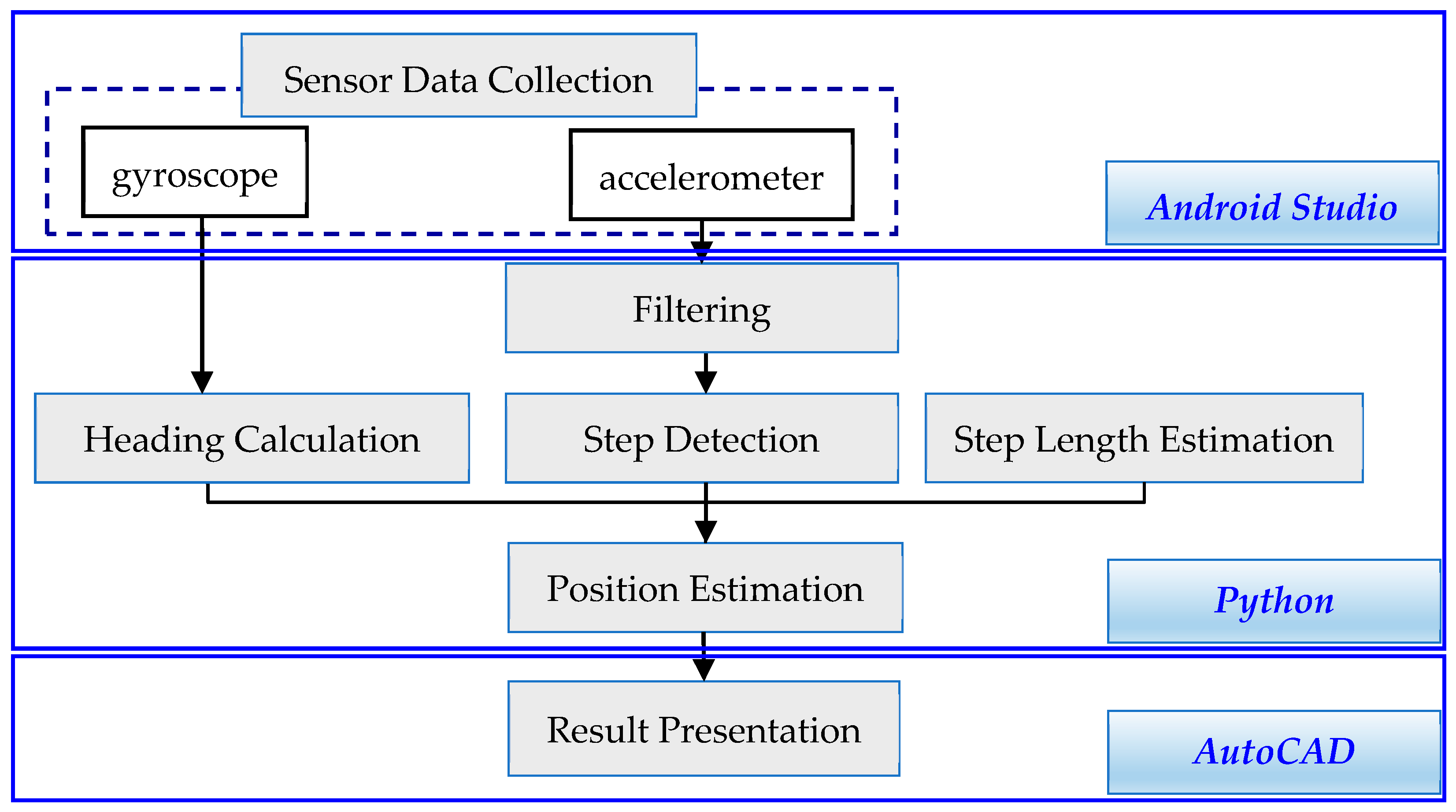
2. Materials and Methods
2.1. Pedestrian Dead Reckoning
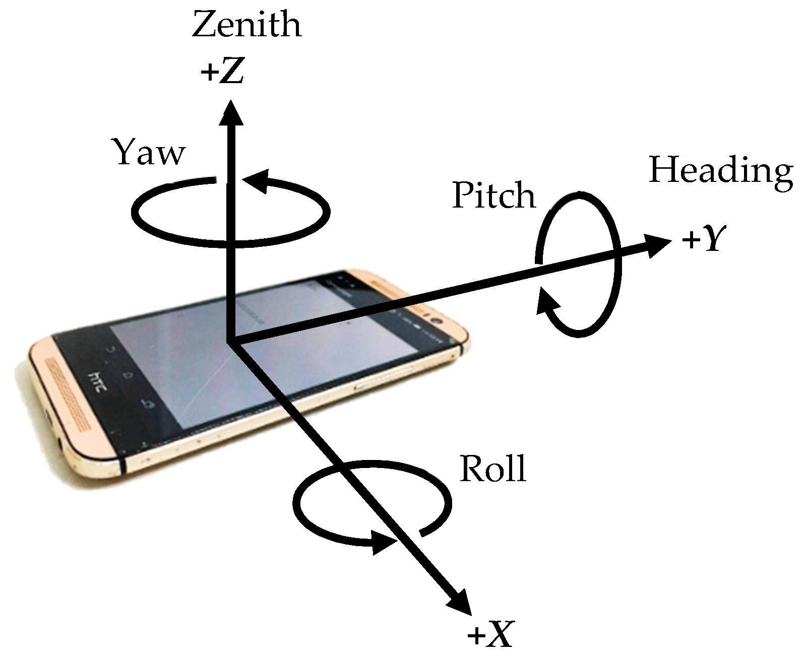
2.1.1. Heading Calculation
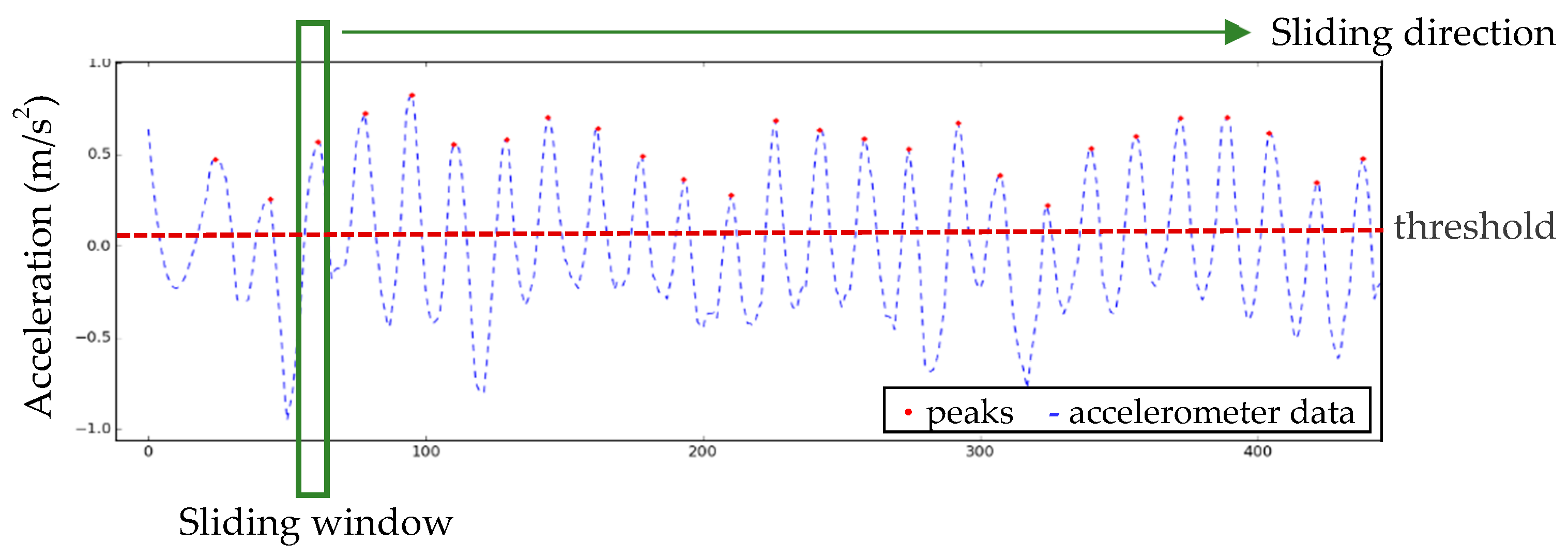
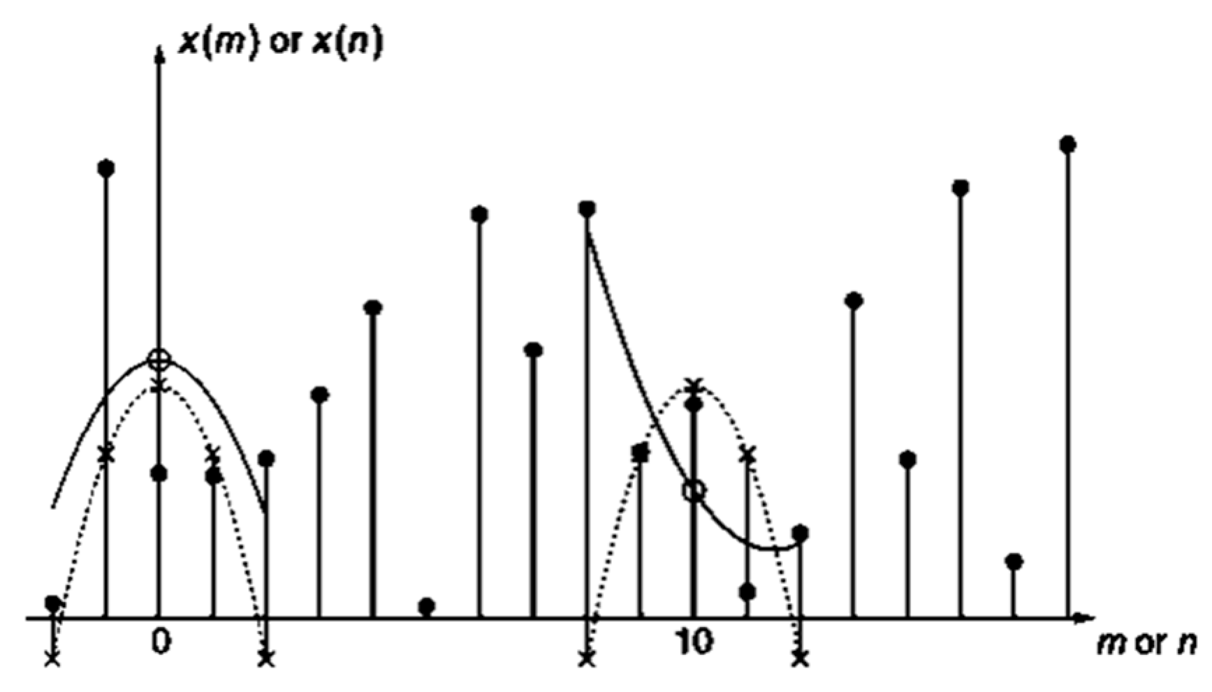
2.1.2. Step Detection and Step Length Estimation
2.2. Establishing a Basic Map
2.3. PDR Correction
2.3.1. Establishing the Calibration Points
2.3.2. Distance Detection
2.3.3. Azimuth Detection
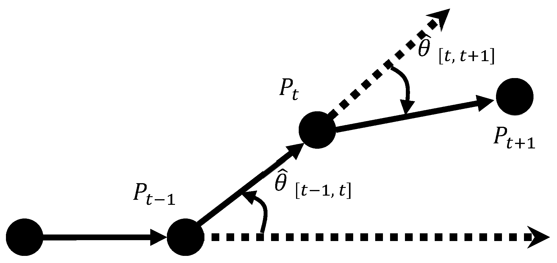
2.3.4. Rotation Angle Detection
3. Results and Discussion
3.1. PDR Positioning
3.2. PDR Correction Positioning
4. Conclusions
- The built-in sensors in the phone and PDR acquired the basic number of steps and navigation data for calculating positions, but the estimation results produced major errors due to propagation errors and low sensor accuracy. The paths calculated through the sensors alone differed significantly from the actual paths, and the relative closure accuracy was only 1/1.5. Therefore, calibration conditions must be applied to PDR for subsequent positioning calculation.
- Known indoor maps were successfully implemented for setting the calibration points, which were divided into corner and linear calibration points. Thresholds and conditions were established according to the characteristics of these points, which assisted in calibrating the PDR positioning results and improving their resemblance to the actual paths.
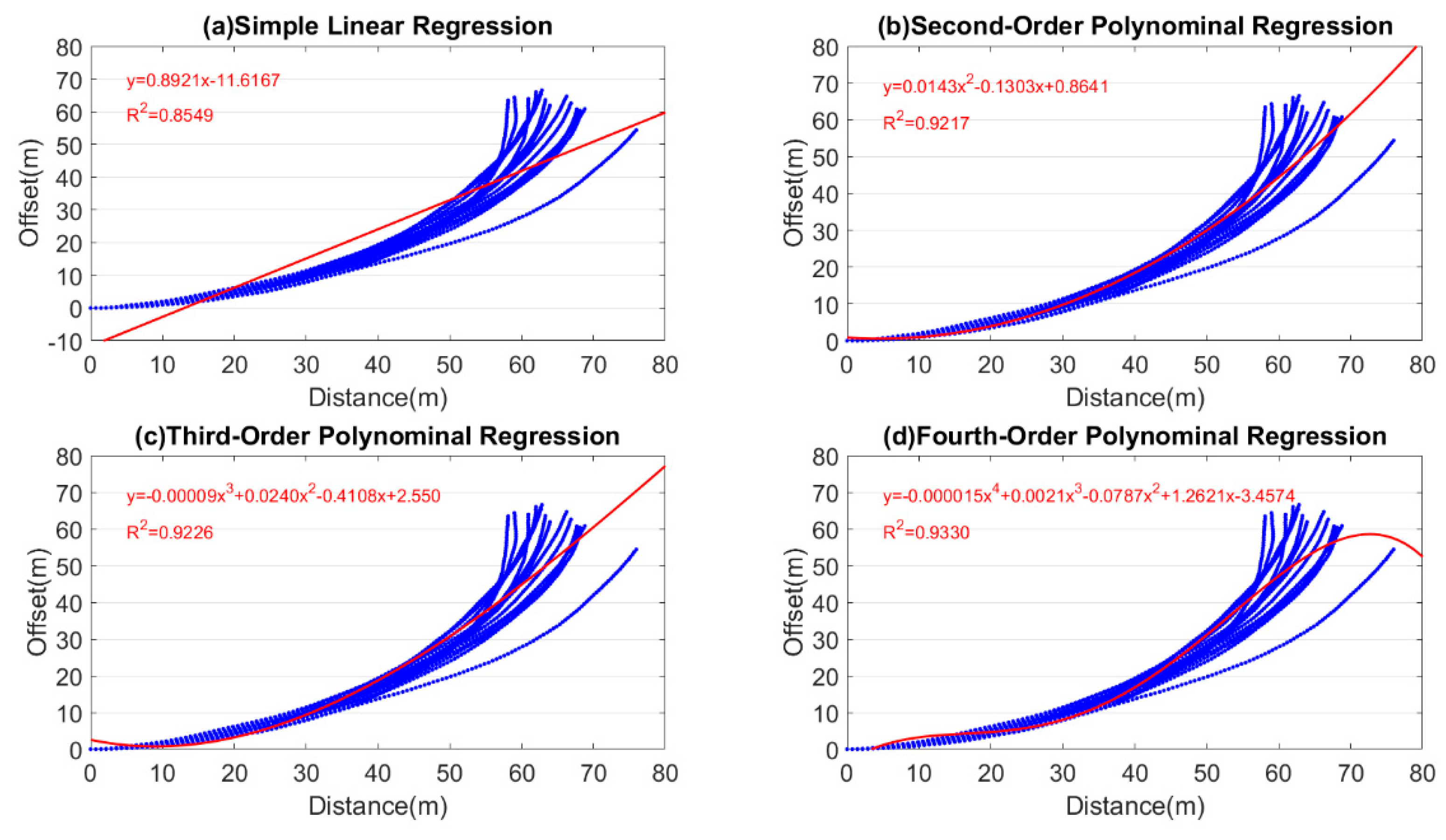
- Regression analysis was successfully performed to calculate the minimal layout intervals between linear calibration points, thereby minimizing the number of control points required in indoor positioning. In addition, this study proved that linear or other regressions were not the most suitable for mobile phone sensor data, but quadratic regression.
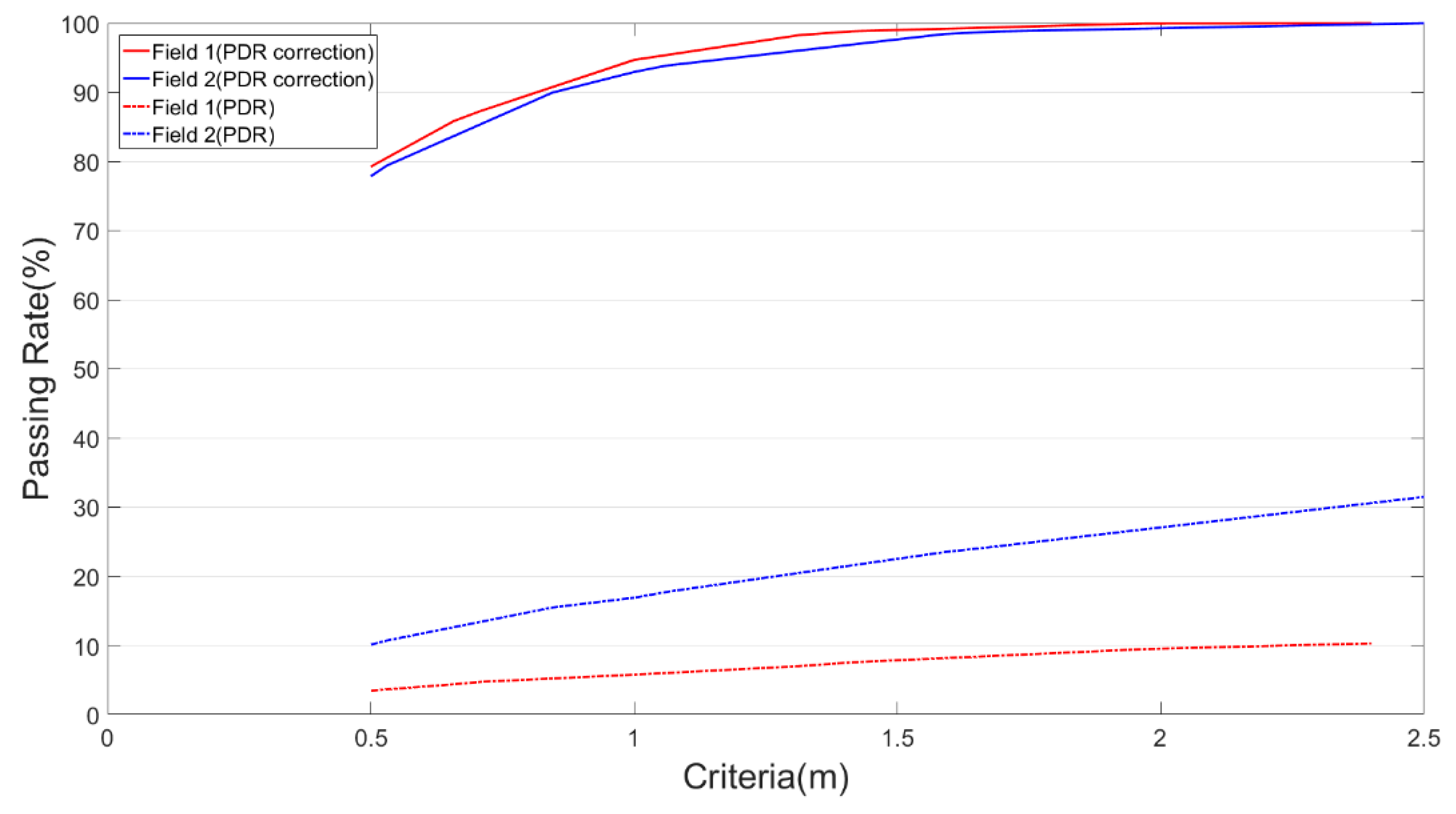
- Establishing calibration points according to known map information was verified to enhance the closeness of the PDR positioning results to the actual paths. The accuracy of the PDR results improved by 95%, and exhibited a root mean square error of 0.6 m after calibration. Moreover, 94% of the calibrated data exhibited errors of <1 m, revealing a desk-level positioning accuracy.
Author Contributions
Funding
Conflicts of Interest
References
- Mautz, R. Indoor Positioning Technologies. Habilitation Thesis, ETH Zurich, Zurich, Switzerland, 2012. [Google Scholar]
- Pelant, J.; Tlamsa, Z.; Benes, V.; Polak, L.; Kaller, O.; Bolecek, L.; Kufa, J.; Sebesta, J.; Kratochvil, T. BLE device indoor localization based on RSS fingerprinting mapped by propagation modes. In Proceedings of the 27th International Conference on Radioelektronika (RADIOELEKTRONIKA), Brno, Czech Republic, 19–20 April 2017; pp. 1–5. [Google Scholar]
- Liu, H.; Darabi, H.; Banerjee, P.; Liu, J. Survey of Wireless Indoor Positioning Techniques and Systems. IEEE Tran. Syst. Man Cybern.—Part C Appl. Rev. 2007, 37, 1067–1080. [Google Scholar] [CrossRef]
- Ni, L.M.; Liu, Y.; Lau, Y.C.; Patil, A.P. LANDMARC: Indoor location sensing using active RFID. In Proceedings of the 1st IEEE International Conference on Pervasive Computing and Communications 2003 (PerCom 2003), Fort Worth, TX, USA, 26 March 2003; pp. 1–9. [Google Scholar]
- Du, Y.; Yang, D.; Xiu, C. A novel method for constructing a WiFi positioning system with efficient manpower. Sensors 2015, 15, 8358–8381. [Google Scholar] [CrossRef] [PubMed]
- Jan, S.S.; Yeh, S.J.; Liu, Y.W. Received signal strength database interpolation by kriging for a Wi-Fi indoor positioning system. Sensors 2015, 15, 21377–21393. [Google Scholar] [CrossRef] [PubMed]
- Ma, L.; Xu, Y. Received signal strength recovery in green WLAN indoor positioning system using singular value thresholding. Sensors 2015, 15, 1292–1311. [Google Scholar] [CrossRef] [PubMed]
- Ma, R.; Guo, Q.; Hu, C.; Xue, J. An improved WiFi indoor positioning algorithm by weighted fusion. Sensors 2015, 15, 21824–21843. [Google Scholar] [CrossRef] [PubMed]
- Caso, G.; Le, M.T.P.; Nardis, L.D.; Benedetto, M.D. Performance comparison of WiFi and UWB fingerprinting indoor positioning systems. Technologies 2018, 6, 14. [Google Scholar] [CrossRef]
- Blumenthal, J.; Grossmann, R.; Golatowski, F.; Timmermann, D. Weighted centroid localization in Zigbee-based Sensor Networks. In Proceedings of the 2007 IEEE International Conference on Intelligent Signal Processing, Alcala de Henares, Spain, 3–5 October 2007; pp. 1–6. [Google Scholar]
- Bianchi, V.; Ciampolini, P.; De Munari, I. RSSI-Based Indoor Localization and Identification for ZigBee Wireless Sensor Networks in Smart Homes. IEEE Trans. Instrum. Meas. 2018, 1–10. [Google Scholar] [CrossRef]
- Yu, K.; Oppermann, I. UWB positioning for wireless embedded networks. In Proceedings of the 2004 IEEE Radio and Wireless Conference (IEEE Cat. No.04TH8746), Atlanta, GA, USA, 22 September 2004; pp. 459–462. [Google Scholar]
- Yua, K.; Montilleta, J.; Rabbachin, A.; Cheonga, P.; Oppermann, I. UWB location and tracking for wireless embedded networks. Signal Process. 2006, 86, 2153–2171. [Google Scholar] [CrossRef]
- El-Sheimy, N.; Niu, X. The promise of MEMS to the navigation community. Inside GNSS 2007, 2, 46–56. [Google Scholar]
- Abdel-Hamid, W. Accuracy Enhancement of Integrated MEMS-IMU/GPS Systems for Land Vehicular Navigation Applications. PhD Thesis, University of Calgary, Calgary, AB, Canada, 2004. [Google Scholar]
- Renaudin, V.; Combettes, C. Magnetic, acceleration fields and gyroscope quaternion (MAGYQ) based attitude estimation with smartphone sensors for indoor pedestrian navigation. Sensors 2014, 14, 22864–22890. [Google Scholar] [CrossRef]
- Castañón–Puga, M.; Salazar, A.S.; Aguilar, L.; Gaxiola-Pacheco, C.; Licea, G. A novel hybrid intelligent indoor location method for mobile devices by zones using Wi-Fi signals. Sensors 2015, 15, 30142–30164. [Google Scholar] [CrossRef] [PubMed]
- Deng, Z.-A.; Wang, G.; Hu, Y.; Wu, D. Heading estimation for indoor pedestrian navigation using a smartphone in the Pocket. Sensors 2015, 15, 21517–21536. [Google Scholar] [CrossRef] [PubMed]
- Xu, Z.; Wei, J.; Zhang, B.; Yang, W. A robust method to detect zero velocity for improved 3D personal navigation using inertial sensors. Sensors 2015, 15, 7708–7727. [Google Scholar] [CrossRef] [PubMed]
- Wang, B.; Liu, X.; Yu, B.; Jia, R.; Gan, X. Pedestrian Dead Reckoning Based on Motion Mode Recognition Using a Smartphone. Sensors (Basel) 2018, 18, 1811. [Google Scholar] [CrossRef] [PubMed]
- Liao, J.K.; Chiang, K.W.; Zhou, Z.M.; Li, Z.H. Using the on-line smoothing and constraint algorithms to improve the accuracy of pedestrian indoor navigation. J. Photogramm. Remote Sens. 2016, 21, 107–123. [Google Scholar]
- Ali, A.S.; Siddharth, S.; El-Sheimy, N.; Syed, Z.F. An improved personal dead-reckoning algorithm for dynamically changing smartphone user modes. In Proceedings of the 25th International Technical Meeting of the Satellite Division of the Institute of Navigation (ION GNSS 2012), Nashville, TN, USA, 17–21 September 2012; pp. 2432–2439. [Google Scholar]
- Ning, F.S.; Wu, D.C. The study of using smart mobile device for step length estimation and step detection. Taiwan J. Geoinform. 2013, 4, 103–116. [Google Scholar]
- Lee-Fang Anga, J.; Lee, W.-K.; Ooi, B.-Y.; Wei-Min Ooi, T.; Hwang, S.O. Pedestrian Dead Reckoning with correction points for indoor positioning and Wi-Fi fingerprint mapping. J. Intell. Fuzzy Syst. 2018. [Google Scholar] [CrossRef]
- Tateno, S.; Cho, Y.; Li, D.; Tian, H.; Hsiao, P. Improvement of pedestrian dead reckoning by heading correction based on optimal access points selection method. In Proceedings of the 2017 56th Annual Conference of the Society of Instrument and Control Engineers of Japan (SICE), Kanazawa, Japan, 19–22 September 2017. [Google Scholar] [CrossRef]
- Kantar. iPhone X Lifts Apple’s Market Share in Spain, Germany and China, 30 January 2018. Available online: https://www.gsmarena.com/kantar_iphone_x_lifts_apples_sales_in_spain_germany_and_china-news-29383.php (accessed on 18 July 2018).
- Shin, S.H.; Park, C.G.; Kim, J.W.; Hong, H.S.; Lee, J.M. Adaptive step length estimation algorithm using Low-Cost MEMS inertial sensors. In Proceedings of the 2007 IEEE Sensors Applications Symposium, San Diego, CA, USA, 6–8 February 2007; pp. 1–5. [Google Scholar]
- Jayalath, S.; Abhayasinghe, N. A gyroscopic data based pedometer algorithm. In Proceedings of the International Conference on Computer Science & Education, Colombo, Sri Lanka, 26–28 April 2013; pp. 551–555. [Google Scholar]
- Kappi, J.; Syrjarinne, J.; Saarinen, J. MEMS-IMU based pedestrian navigator for handheld devices. In Proceedings of the 14th International Technology Meeting of the Satellite Division of the Institute of Navigation ION GPS, Salt Lake City, UT, USA, 11–14 September 2001. [Google Scholar]
- Ailisto, H.J.; Lindholm, M.J.; Mantyjarvi, J.; Vildjiounaite, E.; Makela, S.-M. Identifying people from gait pattern with accelerometers. In Proceedings of the SPIE 5779, Biometric Technology for Human Identification II, Orlando, FL, USA, 28 March 2005. [Google Scholar]
- Rai, A.; Chintalapudi, K.K.; Padmanabhan, V.N.; Sen, R.Z. Zero-effort crowdsourcing for indoor localization. In Proceedings of the 18th Annual International Conference on Mobile Computing and Networking, Istanbul, Turkey, 22–26 August 2012; pp. 293–304. [Google Scholar]
- Ying, H.; Silex, C.; Schnitzer, A.; Leonhardt, S.; Schiek, M. Automatic step detection in the accelerometer signal. In Proceedings of the 4th International Workshop on Wearable and Implantable Body Sensor Networks (BSN 2007), Aachen, Germany, 26–28 March 2007; Springer: Berlin/Heidelberg, Germany; pp. 80–85. [Google Scholar]
- Zhao, X.; Syed, Z.; Wright, D.B.; El-Sheimy, N. An economical and effective multi sensor integration for portable navigation system. In Proceedings of the 22nd International Technical Meeting of the Satellite Division of the Institute of Navigation (ION GNSS 2009), Savsannah, GA, USA, 22–25 September 2009; pp. 2088–2095. [Google Scholar]
- Lan, K.C.; Shih, W.Y. Using smart-phones and floor plans for indoor location tracking. IEEE Trans. Hum. Mach. Syst. 2014, 44, 211–221. [Google Scholar]
- Chen, G.L.; Fei, L.I.; Zhang, Y.Z. Pedometer method based on adaptive peak detection algorithm. J. Chin. Inertial Technol. 2015, 23, 315–321. [Google Scholar]
- Yang, X.; Huang, B. An accurate step detection algorithm using unconstrained smartphones. In Proceedings of the 27th Chinese Control and Decision Conference, Qingdao, China, 23–25 May 2015; pp. 5682–5687. [Google Scholar]
- Savitzky, A.; Golay, M.J.E. Soothing and differentiation of data by simplified least squares procedures. Anal. Chem. 1964, 36, 1627–1639. [Google Scholar] [CrossRef]
- Riordon, J.; Zubritsky, E.; Newman, A. Top 10 articles. Anal. Chem. 2000, 72, 324A–329A. [Google Scholar] [CrossRef] [PubMed]
- Schafer, R.W. What Is a savitzky-golay filter? IEEE Signal Process. Mag. 2011, 28, 111–117. [Google Scholar] [CrossRef]
- Geospatial World. Indoor Positioning: What Do You Do in a Building When Your GPS Stops Working? Available online: https://www.geospatialworld.net/blogs/indoor-positioning-indoors-gps-stops-working/ (accessed on 10 November 2018).

 start point;
  end point;
  calibration point on the corner;
  true path.)
start point; end point; calibration point on the corner; true path.)
true path.)
start point; end point; calibration point on the corner; true path.)
 calibration point;
  sensor point;
  true path;
  sensor path.)
calibration point; sensor point; true path; sensor path.)
sensor path.)
calibration point; sensor point; true path; sensor path.)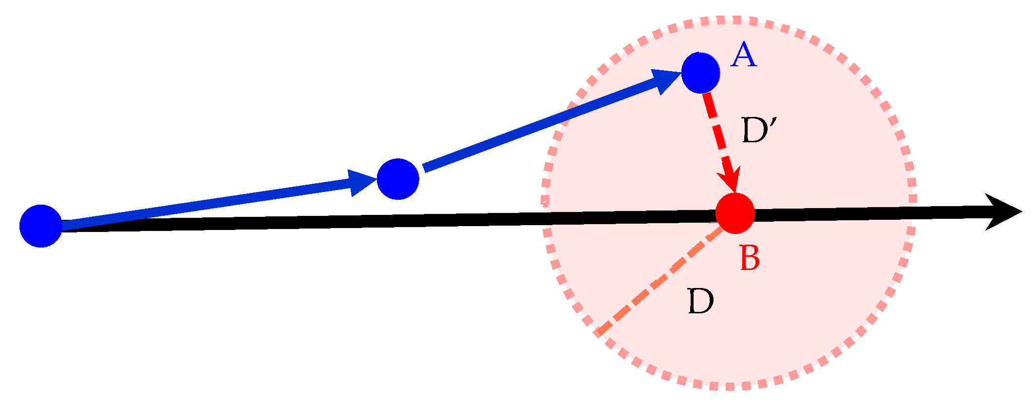 calibration point; sensor point; true path; sensor path.)
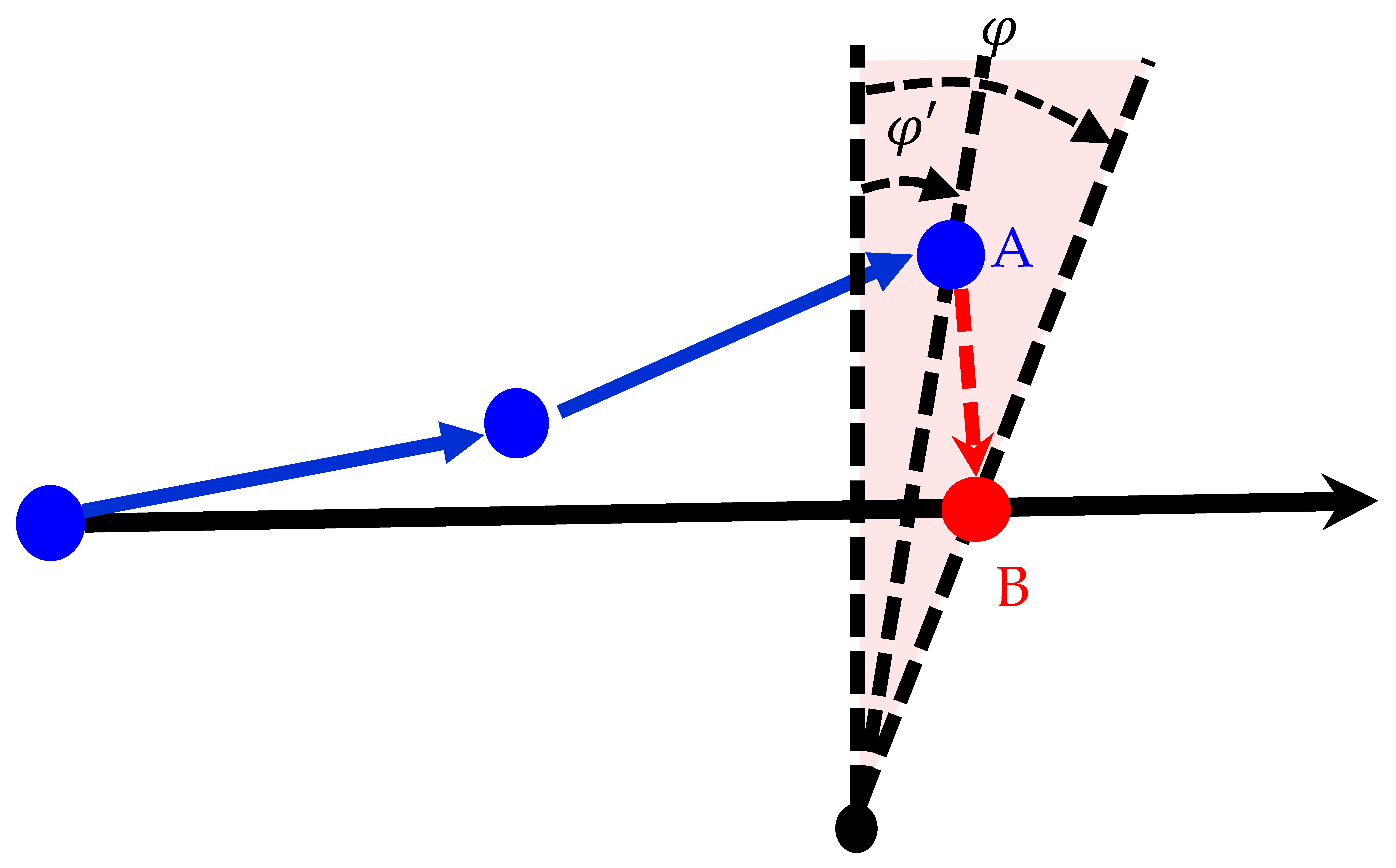 calibration point; sensor point;
  path before calibration;
  path after calibration.)
calibration point; sensor point; path before calibration; path after calibration.)
path after calibration.)
calibration point; sensor point; path before calibration; path after calibration.)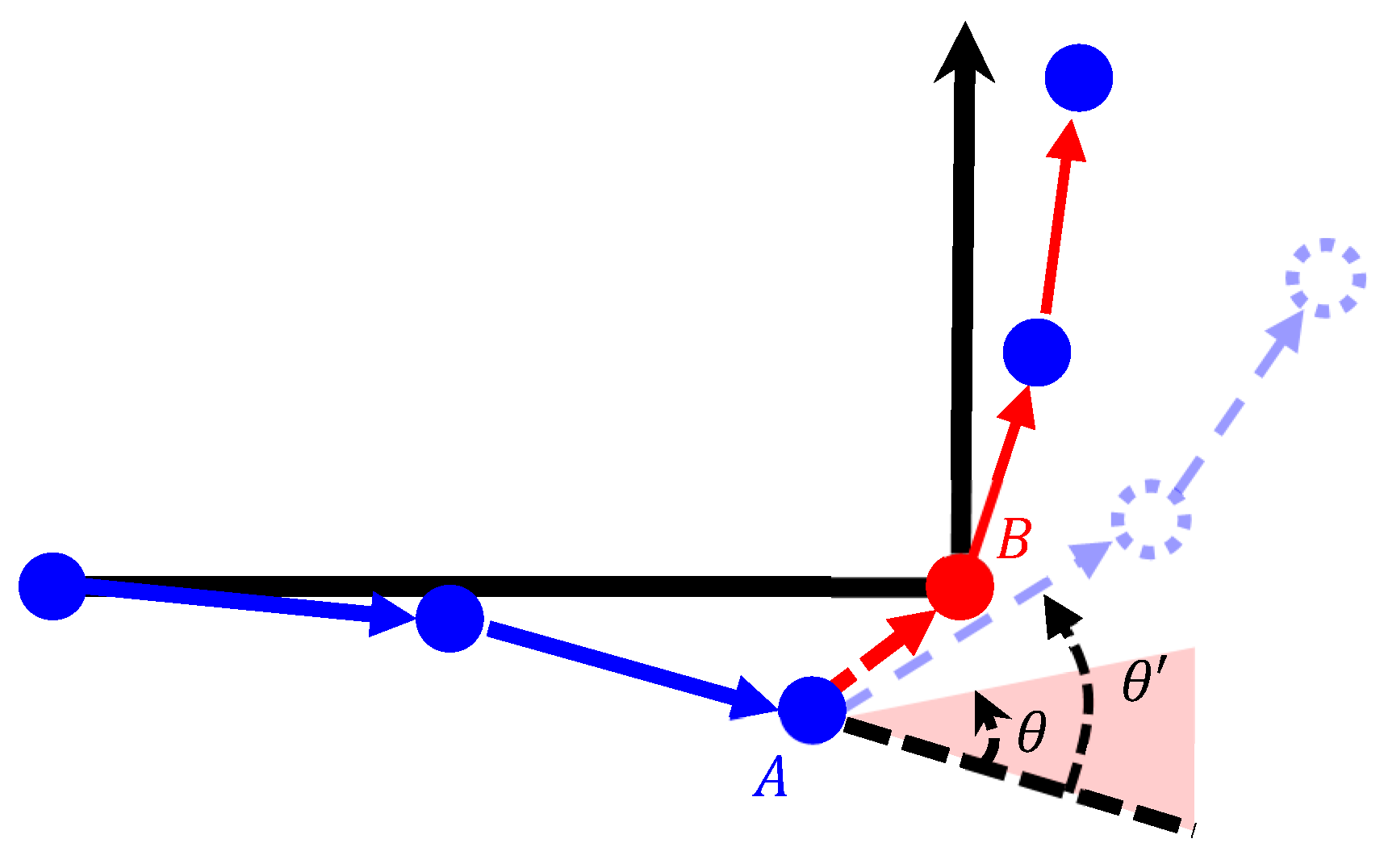 calibration point; sensor point; path before calibration; path after calibration.)
calibration point; sensor point; path before calibration; path after calibration.)
calibration point; sensor point; path before calibration; path after calibration.)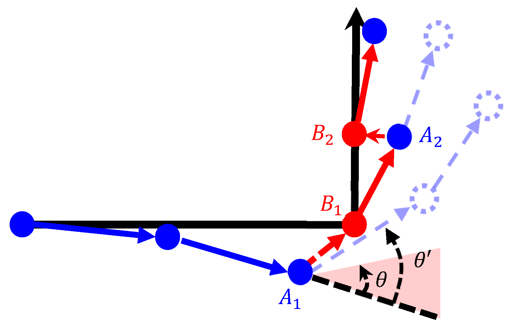 start point; end point; true path;
  PDR path.)
start point; end point; true path; PDR path.)
PDR path.)
start point; end point; true path; PDR path.)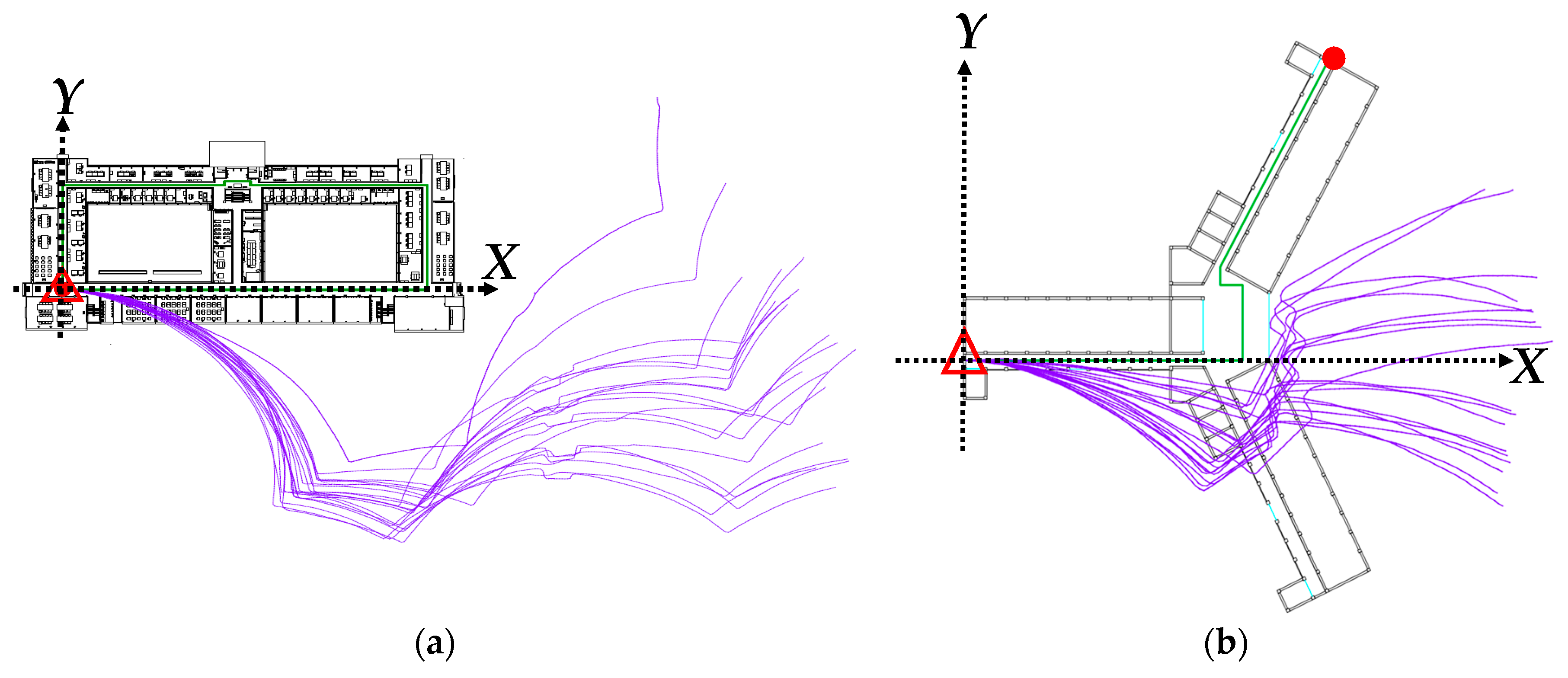 start point; end point;
  calibration point on the line; calibration point on the corner; corrected PDR path.)
start point; end point; calibration point on the line; calibration point on the corner; corrected PDR path.)
calibration point on the line; calibration point on the corner; corrected PDR path.)
start point; end point; calibration point on the line; calibration point on the corner; corrected PDR path.)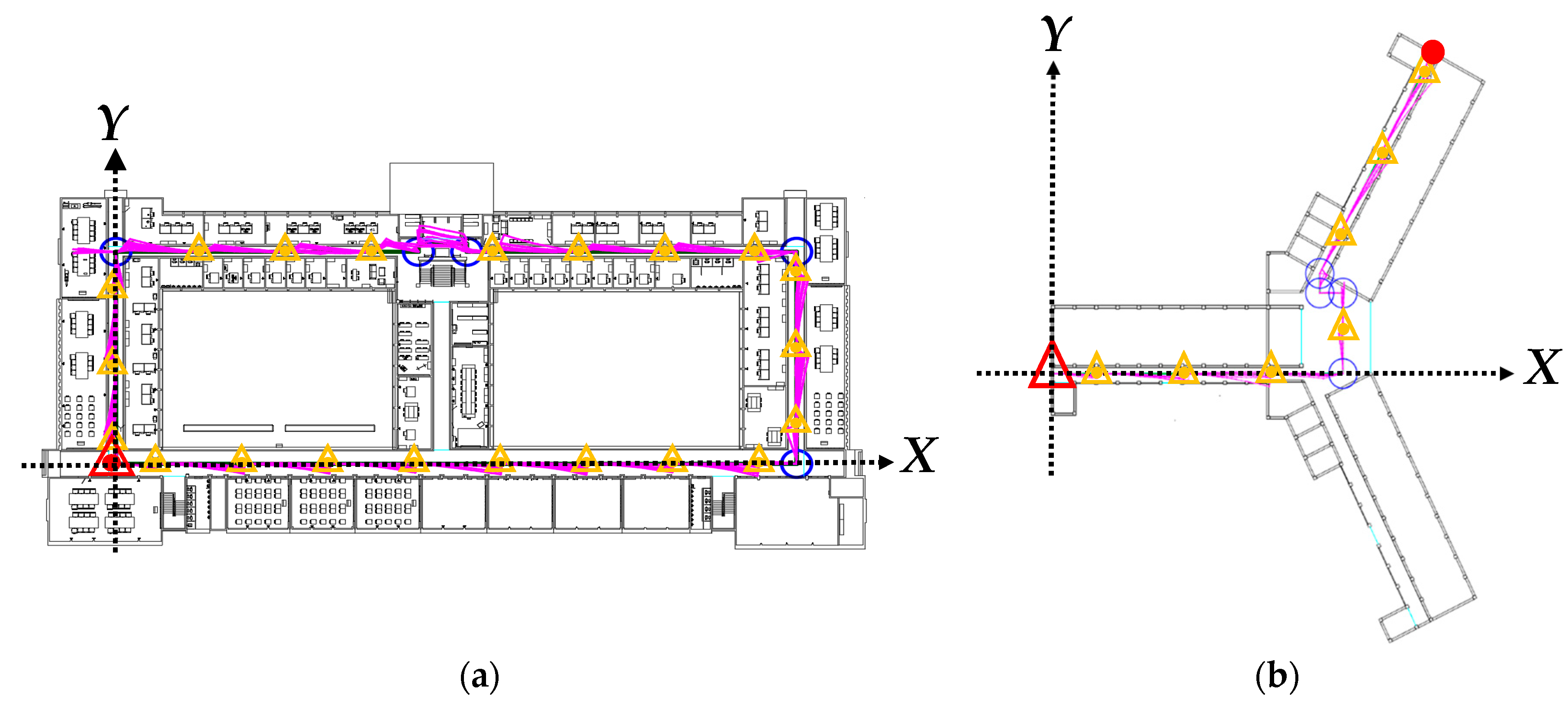 sensor point; true path; sensor path.)
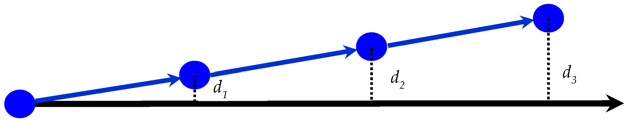

| Technology | Frequency | Accuracy | Advantages | Disadvantages |
|---|---|---|---|---|
| Bluetooth/ iBeacon | 2.4 GHz | cm–m |
|
|
| IR | None | cm |
|
|
| RFID | 125 KHz/ Hundreds of MHz | dm–m |
|
|
| Wi-Fi | 2.4 GHz | m |
|
|
| Zigbee | 2.4 GHz | m |
|
|
| UWB | 3–10 GHz | cm |
|
|
| System | Processor | Sensing Device |
|---|---|---|
| Android 6.0 | Qualcomm® Snapdragon 801, Quad core processor | Accelerometer, Gyroscope, Gravity sensor. |
| Path | Field 1 | Field 2 |
|---|---|---|
| Type | Closed | Connecting |
| Length | 245 m | 92 m |
| Narrowest width | 1.4 m | 1.7 m |
| Number of turns | 5 | 4 |
| Closure | MAX | MIN | MEAN | RMSE | Relative Accuracy | |
|---|---|---|---|---|---|---|
| Field 1 | ΔX | 196.175 | 147.390 | 182.287 | 182.643 | 1/1.342 |
| ΔY | 57.313 | 0.144 | 24.988 | 32.085 | 1/7.638 | |
| 2D | 201.856 | 158.189 | 185.092 | 185.440 | 1/1.321 | |
| Field 2 | ΔX | 26.834 | 14.480 | 24.067 | 24.162 | 1/3.762 |
| ΔY | 70.514 | 19.545 | 45.719 | 47.715 | 1/1.905 | |
| 2D | 73.496 | 26.899 | 52.019 | 53.484 | 1/1.720 | |
| Closure | MAX | MIN | MEAN | RMSE | Relative Accuracy | |
|---|---|---|---|---|---|---|
| Field 1 | ΔX | 0.162 | 0.004 | 0.086 | 0.100 | 1/2444.525 |
| ΔY | 1.042 | 0.067 | 0.558 | 0.649 | 1/377.532 | |
| 2D | 1.051 | 0.072 | 0.570 | 0.657 | 1/373.109 | |
| Field 2 | ΔX | 0.621 | 0.032 | 0.244 | 0.303 | 1/299.709 |
| ΔY | 0.944 | 0.032 | 0.365 | 0.435 | 1/209.054 | |
| 2D | 1.130 | 0.121 | 0.455 | 0.530 | 1/171.463 | |
| Type | Field | Criteria (m) | Passing Rate of PDR (%) | Passing Rate of PDR Correction (%) |
|---|---|---|---|---|
| 1/2 Desk level | Field 1 | 0.500 | 3.462 | 79.248 |
| Field 2 | 0.500 | 10.120 | 77.860 | |
| 1σ of corrected closure | Field 1 | 0.657 | 4.373 | 85.824 |
| Field 2 | 0.530 | 10.698 | 79.389 | |
| 1/2 Aisle width | Field 1 | 0.708 | 4.722 | 87.280 |
| Field 2 | 0.845 | 15.489 | 89.963 | |
| Desk level | Field 1 | 1.000 | 5.770 | 94.688 |
| Field 2 | 1.000 | 16.894 | 92.937 | |
| 2σ of corrected closure | Field 1 | 1.314 | 7.000 | 98.272 |
| Field 2 | 1.060 | 17.720 | 93.846 | |
| Aisle width | Field 1 | 1.416 | 7.561 | 98.832 |
| Field 2 | 1.690 | 24.329 | 98.802 | |
| 3σ of corrected closure | Field 1 | 1.971 | 9.475 | 99.968 |
| Field 2 | 1.590 | 23.503 | 98.430 | |
| All pass | Field 1 | 2.4000 | 10.295 | 100.000 |
| Field 2 | 2.5000 | 31.475 | 100.000 |
© 2018 by the authors. Licensee MDPI, Basel, Switzerland. This article is an open access article distributed under the terms and conditions of the Creative Commons Attribution (CC BY) license (http://creativecommons.org/licenses/by/4.0/).
Share and Cite
Li, Y.-S.; Ning, F.-S. Low-Cost Indoor Positioning Application Based on Map Assistance and Mobile Phone Sensors. Sensors 2018, 18, 4285. https://doi.org/10.3390/s18124285
Li Y-S, Ning F-S. Low-Cost Indoor Positioning Application Based on Map Assistance and Mobile Phone Sensors. Sensors. 2018; 18(12):4285. https://doi.org/10.3390/s18124285
Chicago/Turabian StyleLi, Yi-Shan, and Fang-Shii Ning. 2018. "Low-Cost Indoor Positioning Application Based on Map Assistance and Mobile Phone Sensors" Sensors 18, no. 12: 4285. https://doi.org/10.3390/s18124285
APA StyleLi, Y.-S., & Ning, F.-S. (2018). Low-Cost Indoor Positioning Application Based on Map Assistance and Mobile Phone Sensors. Sensors, 18(12), 4285. https://doi.org/10.3390/s18124285