RECRP: An Underwater Reliable Energy-Efficient Cross-Layer Routing Protocol †

Abstract
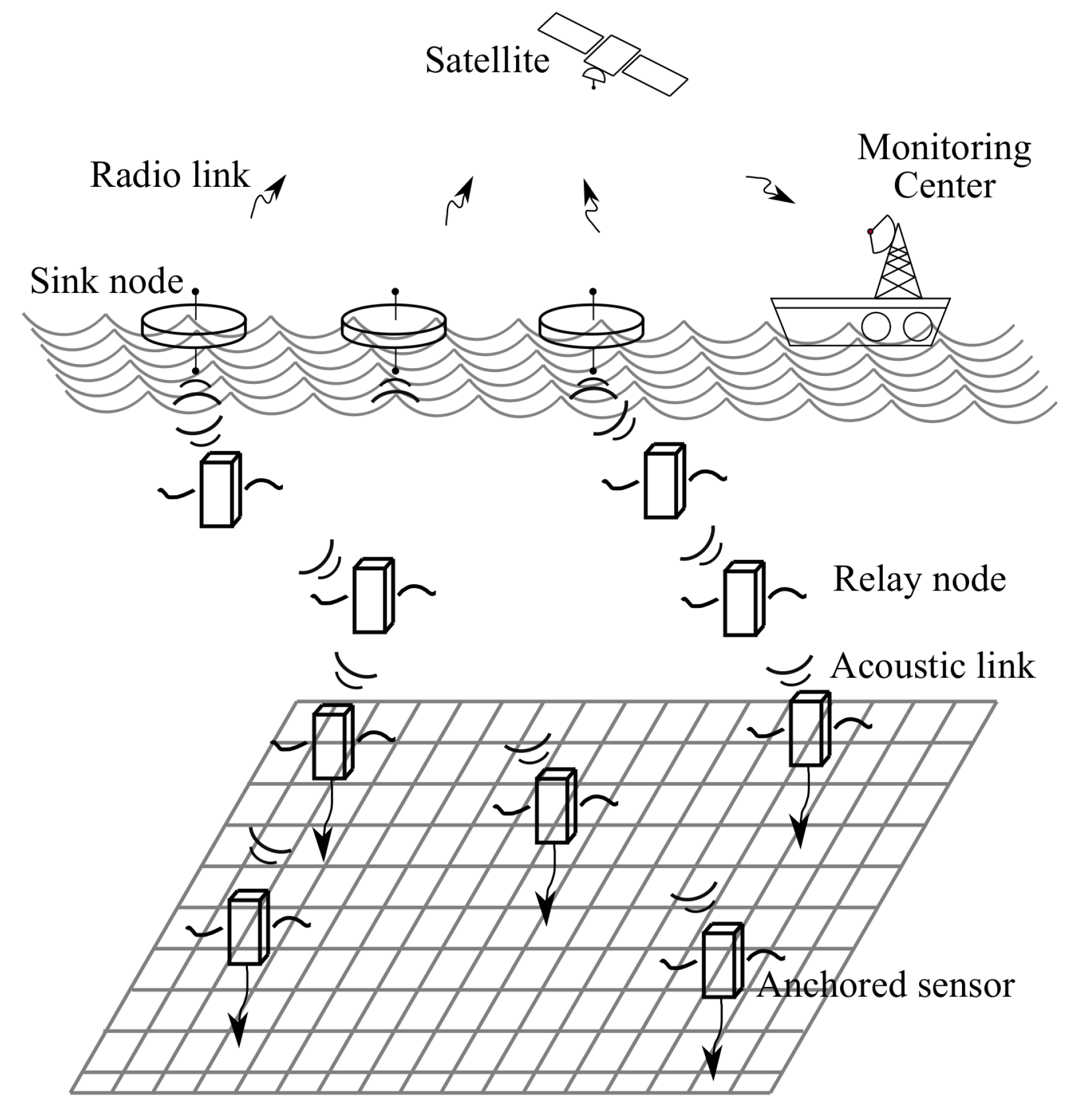
1. Introduction
- We propose a location-free single-copy routing protocol, RECRP, to deal with the high energy consumption and imbalanced energy cost in underwater sensor networks. We use the mixed integer linear programming (MILP) model with a max–min method to formulate the underwater routing forwarding problem to achieve energy efficiency. The protocol also handles the communication void problem, which is a common problem in greedy routing protocols.
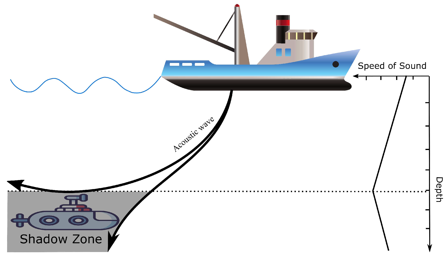
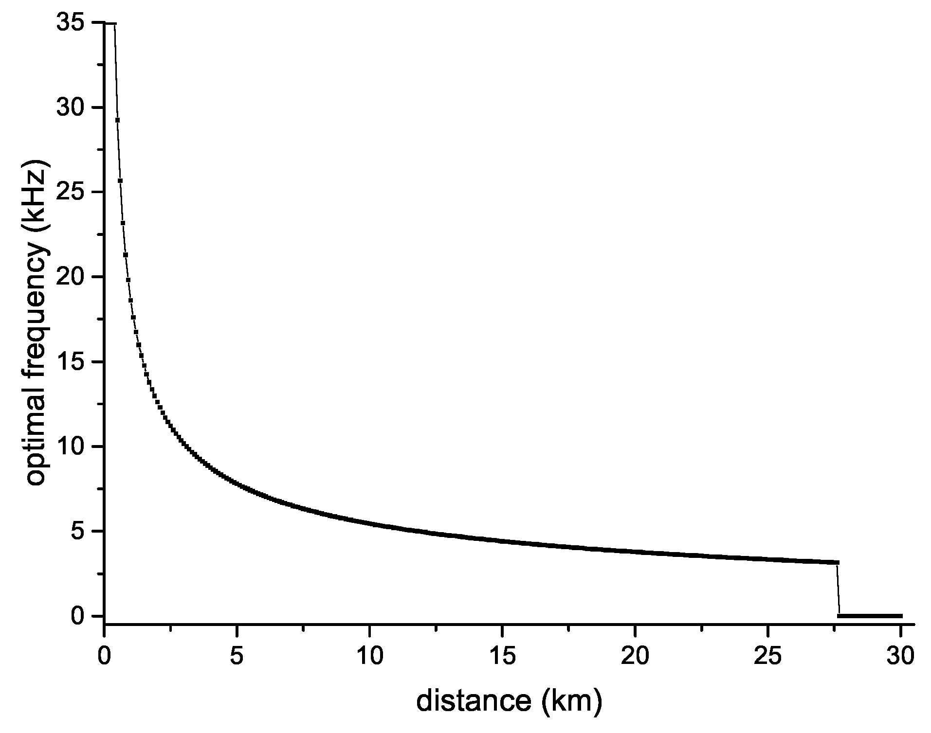
- We adopt the information of physical layer such as Doppler scale shift measurement and RSSI to estimate the relative velocity and distance without extra hardware to make RECRP suitable for many underwater scenarios.
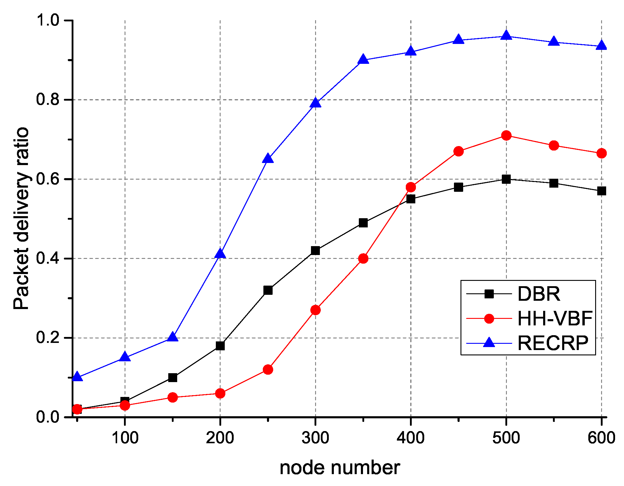
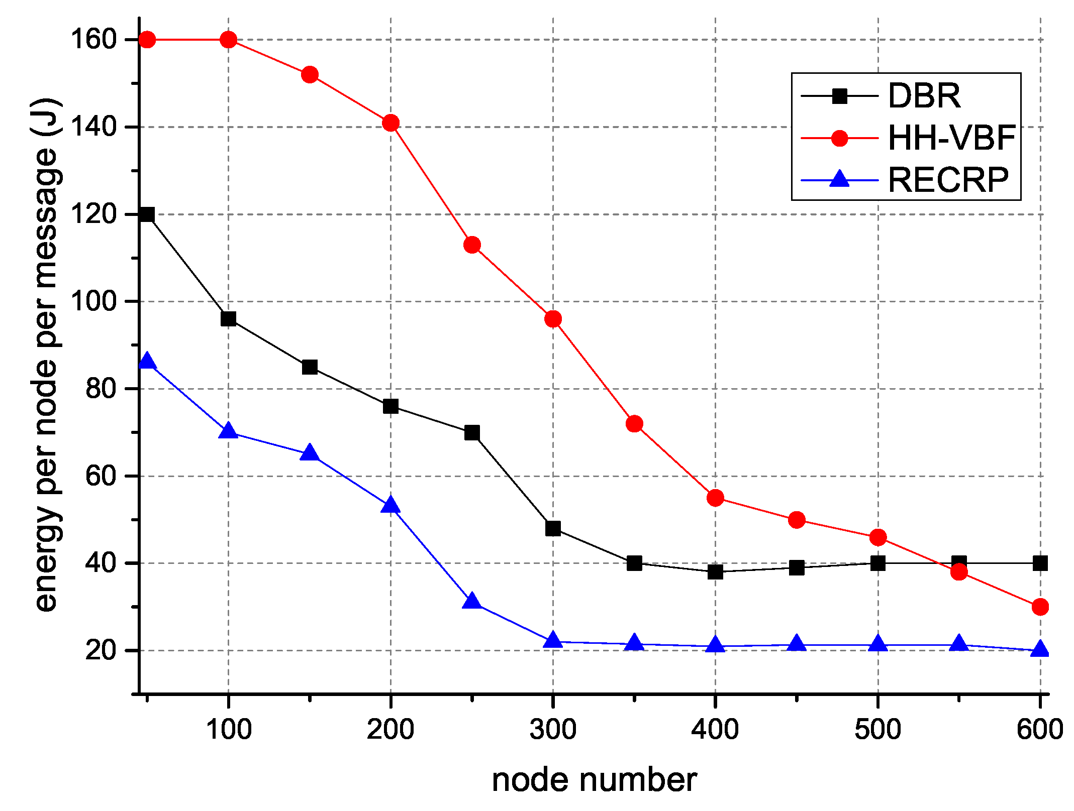
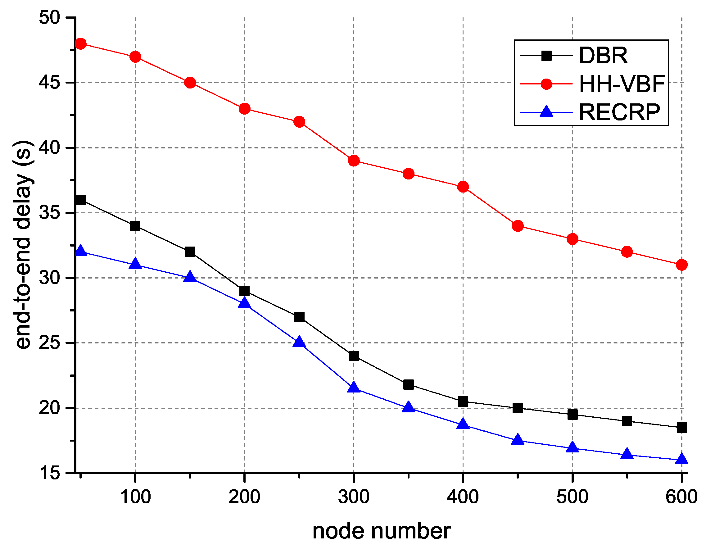
- We conducted simulations to verify the performance of RECRP in a randomly deployed sparse network. Simulation results show that in terms of packet delivery rate, energy consumption, and end-to-end delay, RECRP performed better than depth-based routing (DBR) and hop-by-hop vector-based forwarding (HH-VBF).
2. Related Work
3. RECRP Description
3.1. Routing Updating Phase
3.2. Routing Phase
4. Simulation
4.1. Simulation Setting
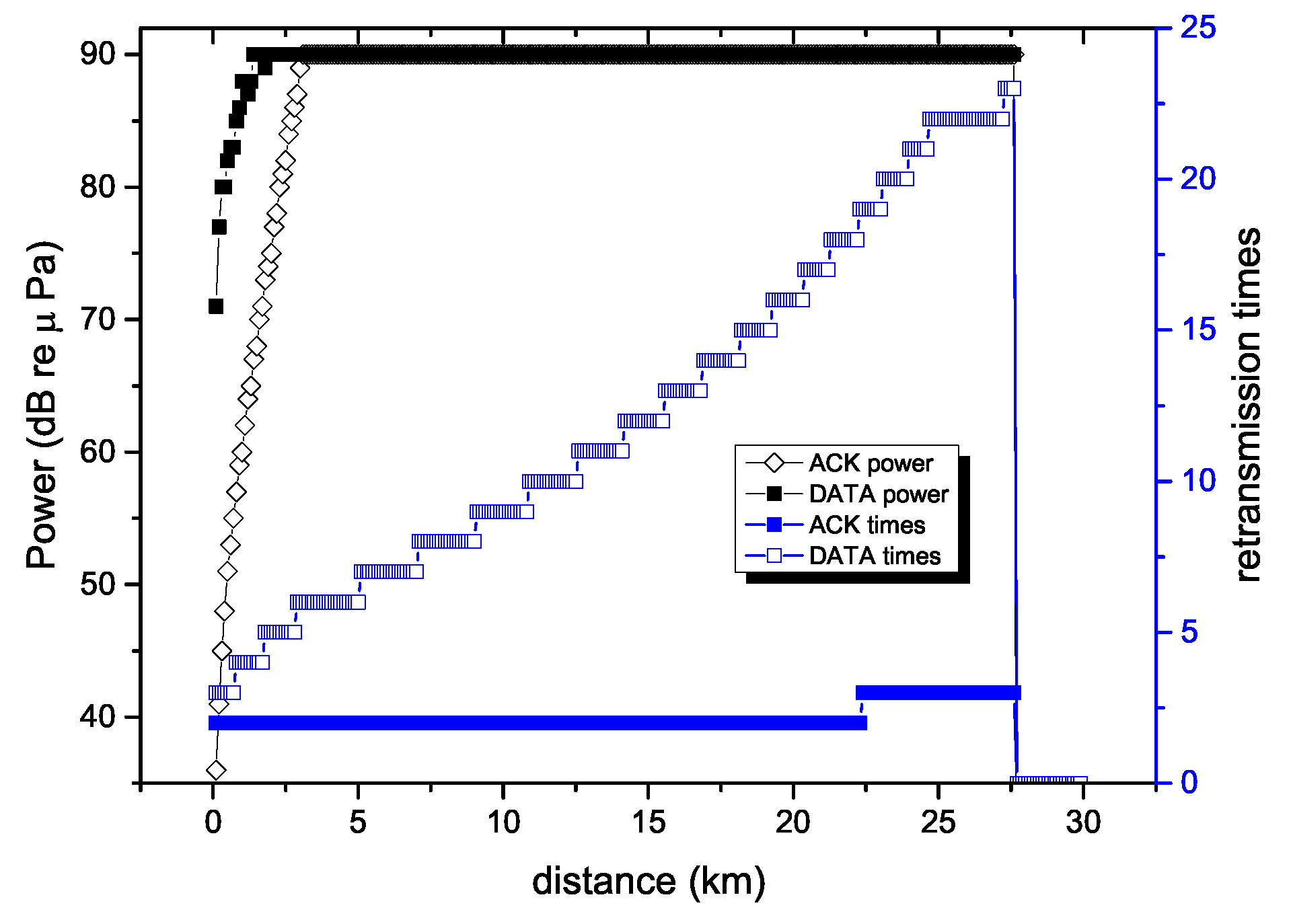
4.2. Results and Analysis
5. Conclusions
Author Contributions
Funding
Conflicts of Interest
References
- Huang, J.G.; Wang, H.; He, C.B.; Zhang, Q.F.; Jing, L.Y. Underwater acoustic communication and the general performance evaluation criteria. Front. Inf. Technol. Electron. Eng. 2018, 19, 951–971. [Google Scholar] [CrossRef]
- Luo, Y.; Pu, L.; Peng, Z.; Zhou, Z.; Cui, J.H.; Zhang, Z. Effective relay selection for underwater cooperative acoustic networks. In Proceedings of the 2013 IEEE 10th International Conference on Mobile Ad-Hoc and Sensor Systems (MASS), Hangzhou, China, 14–16 October 2013; pp. 104–112. [Google Scholar]
- Luo, Y.; Pu, L.; Zuba, M.; Peng, Z.; Cui, J.H. Challenges and opportunities of underwater cognitive acoustic networks. IEEE Trans. Emerg. Top. Comput. 2014, 2, 198–211. [Google Scholar] [CrossRef]
- Wang, X.; Wei, D.; Wei, X.; Cui, J.; Pan, M. HAS4: A Heuristic Adaptive Sink Sensor Set Selection for Underwater AUV-Aid Data Gathering Algorithm. Sensors 2018, 18, 4110. [Google Scholar] [CrossRef] [PubMed]
- Wei, X.; Wang, X.; Bai, X.; Bai, S.; Liu, J. Autonomous underwater vehicles localisation in mobile underwater networks. Int. J. Sens. Netw. 2017, 23, 61–71. [Google Scholar] [CrossRef]
- Ovaliadis, K.; Savage, N.; Kanakaris, V. Energy Efficiency in Underwater Sensor Networks: A Research Review. J. Eng. Sci. Technol. Rev. 2010, 3, 151–156. [Google Scholar] [CrossRef]
- Ayaz, M.; Baig, I.; Abdullah, A.; Faye, I. A survey on routing techniques in underwater wireless sensor networks. J. Netw. Comput. Appl. 2011, 34, 1908–1927. [Google Scholar] [CrossRef]
- Mohamad, M.M.; Kheirabadi, M.T. Greedy Routing in Underwater Acoustic Sensor Networks: A Survey. Int. J. Distrib. Sens. Netw. 2013, 2013, 828–831. [Google Scholar]
- Lu, F.; Mirza, D.; Schurgers, C. D-sync:Doppler-based time synchronization for mobile underwater sensor networks. In Proceedings of the ACM International Workshop on Underwater Networks, Woods Hole, MA, USA, 30 September–1 October 2010; pp. 1–8. [Google Scholar]
- Li, B.; Zhou, S.; Stojanovic, M.; Freitag, L.; Willett, P. Multicarrier Communication Over Underwater Acoustic Channels with Nonuniform Doppler Shifts. IEEE J. Ocean. Eng. 2008, 33, 198–209. [Google Scholar]
- Xie, P.; Cui, J.H.; Lao, L. VBF: Vector-Based Forwarding Protocol for Underwater Sensor Networks. In Lecture Notes in Computer Science; Springer: Coimbra, Portugal, 2006. [Google Scholar]
- Nicolaou, N.; See, A.; Xie, P.; Cui, J.H.; Maggiorini, D. Improving the Robustness of Location-Based Routing for Underwater Sensor Networks. In Proceedings of the OCEANS 2007—Europe, Aberdeen, UK, 18–21 June 2007; pp. 1–6. [Google Scholar]
- Yu, H.; Yao, N.; Liu, J. An Adaptive Routing Protocol in Underwater Sparse Acoustic Sensor Networks; Elsevier Science Publishers B. V.: Amsterdam, The Netherlands, 2015; pp. 121–143. [Google Scholar]
- Coutinho, R.W.L.; Boukerche, A.; Vieira, L.F.M.; Loureiro, A.A.F. GEDAR: Geographic and opportunistic routing protocol with Depth Adjustment for mobile underwater sensor networks. In Proceedings of the IEEE International Conference on Communications, Sydney, Australia, 10–14 June 2014; pp. 251–256. [Google Scholar]
- Coutinho, R.W.L.; Vieira, L.F.M.; Loureiro, A.A.F. DCR: Depth-Controlled Routing protocol for underwater sensor networks. In Proceedings of the International Symposium on Computers and Communications, Split, Croatia, 7–10 July 2013; pp. 453–458. [Google Scholar]
- Yan, H.; Shi, Z.J.; Cui, J.H. DBR: Depth-based routing for underwater sensor networks. In Proceedings of the International Ifip-Tc6 networking Conference on Adhoc and Sensor Networks, Wireless Networks, Next Generation Internet, Singapore, 5–9 May 2008; pp. 72–86. [Google Scholar]
- Liu, G.; Li, Z. Depth-Based Multi-hop Routing protocol for Underwater Sensor Network. In Proceedings of the International Conference on Industrial Mechatronics and Automation, Wuhan, China, 30–31 May 2010; pp. 268–270. [Google Scholar]
- Diao, B.; Xu, Y.; An, Z.; Wang, F.; Li, C. Improving both energy and time efficiency of depth-based routing for underwater sensor networks. Int. J. Distrib. Sens. Netw. 2015, 2015, 8. [Google Scholar] [CrossRef]
- Wahid, A.; Lee, S.; Kim, D. An energy-efficient routing protocol for UWSNs using physical distance and residual energy. In Proceedings of the OCEANS 2011 IEEE—Spain, Santander, Spain, 6–9 June 2011; pp. 1–6. [Google Scholar]
- Ashrafuddin, M.; Islam, M.M.; Mamunorrashid, M. Energy Efficient Fitness Based Routing Protocol for Underwater Sensor Network. Int. J. Intell. Syst. Appl. 2013, 5, 61–69. [Google Scholar] [CrossRef]
- Stojanovic, M. On the relationship between capacity and distance in an underwater acoustic communication channel. ACM Sigmobile Mob. Comput. Commun. Rev. 2007, 11, 34–43. [Google Scholar] [CrossRef]
- Lysanov, Y.P.; Brekhovskikh, L.M. Fundamentals Of Ocean Acoustics; Springer: Berlin, Germany, 1982; pp. 3382–3383. [Google Scholar]
- Brekhovskikh, L.M.; Lysanov, Y.P. Fundamentals of Ocean Acoustics, 2nd ed.; Springer: Berlin, Germany, 1991; pp. 3382–3383. [Google Scholar]
- Chandrasekhar, V.; Seah, W.K.; Choo, Y.S.; Ee, H.V. Localization in underwater sensor networks: Survey and challenges. In Proceedings of the 1st ACM International Workshop on Underwater Networks, Los Angeles, CA, USA, 25 September 2006; pp. 33–40. [Google Scholar]
- Savvides, A.; Han, C.; Strivastava, B.M. Dynamic fine-grained localization in Ad-Hoc networks of sensors. In Proceedings of the 7th Annual International Conference on Mobile Computing and Networking, Rome, Italy, 16–21 July 2001. [Google Scholar]
- Chitre, M.; Potter, J.; Heng, O.S. Underwater acoustic channel characterisation for medium-range shallow water communications. In Proceedings of the Oceans ’04 MTS/IEEE Techno-Ocean ’04, Kobe, Japan, 9–12 November 2004; pp. 40–45. [Google Scholar]
- Mason, S.; Berger, C.R.; Zhou, S.; Willett, P. Detection, Synchronization, and Doppler Scale Estimation with Multicarrier Waveforms in Underwater Acoustic Communication. In Proceedings of the OCEANS 2008—MTS/IEEE Kobe Techno-Ocean, Kobe, Japan, 8–11 April 2008; pp. 1–6. [Google Scholar]
- Coates, R.F.W. Underwater Acoustic Systems; Macmillan Education: London, UK, 1990. [Google Scholar]
- Ghoreyshi, S.M.; Shahrabi, A.; Boutaleb, T. An Underwater Routing Protocol with Void Detection and Bypassing Capability. In Proceedings of the IEEE International Conference on Advanced Information NETWORKING and Applications, Taipei, Taiwan, 27–29 March 2017; pp. 530–537. [Google Scholar]
- Rappaport, T. Wireless Communications: Principles and Practice; Prentice Hall PTR: Upper Saddle River, NJ, USA, 2001; Volume 8, pp. 33–38. [Google Scholar]
- Noh, Y.; Lee, U.; Lee, S.; Wang, P.; Vieira, L.F.M.; Cui, J.H.; Gerla, M.; Kim, K. HydroCast: Pressure Routing for Underwater Sensor Networks. IEEE Trans. Veh. Technol. 2016, 65, 333–347. [Google Scholar] [CrossRef]
- Hamming, R.W. Error Detecting and Error Correcting Codes. Bell Syst. Tech. J. 2014, 29, 147–160. [Google Scholar] [CrossRef]
- Jiang, S. On Reliable Data Transfer in Underwater Acoustic Networks: A Survey from Networking Perspective. IEEE Commun. Surv. Tutor. 2018, 20, 1036–1055. [Google Scholar] [CrossRef]
- Bagtzoglou, A.C.; Andrei, N. Chaotic Behavior and Pollution Dispersion Characteristics in Engineered Tidal Embayments: A Numerical Investigation. Jawra J. Am. Water Resour. Assoc. 2010, 43, 207–219. [Google Scholar]


| ID | Velocity | Distance | Energy | Level | Timer |
|---|---|---|---|---|---|
| 1 | 0.2 | 30 | 1 | 12 | |
| 3 | 15 | 3 | 17 |
| Variable | Value | Variable | Value |
|---|---|---|---|
| k | 1 | ||
| v | m/s |
© 2018 by the authors. Licensee MDPI, Basel, Switzerland. This article is an open access article distributed under the terms and conditions of the Creative Commons Attribution (CC BY) license (http://creativecommons.org/licenses/by/4.0/).
Share and Cite
Liu, J.; Yu, M.; Wang, X.; Liu, Y.; Wei, X.; Cui, J. RECRP: An Underwater Reliable Energy-Efficient Cross-Layer Routing Protocol. Sensors 2018, 18, 4148. https://doi.org/10.3390/s18124148
Liu J, Yu M, Wang X, Liu Y, Wei X, Cui J. RECRP: An Underwater Reliable Energy-Efficient Cross-Layer Routing Protocol. Sensors. 2018; 18(12):4148. https://doi.org/10.3390/s18124148
Chicago/Turabian StyleLiu, Jun, Meiming Yu, Xingwang Wang, Yuanyuan Liu, Xiaohui Wei, and Junhong Cui. 2018. "RECRP: An Underwater Reliable Energy-Efficient Cross-Layer Routing Protocol" Sensors 18, no. 12: 4148. https://doi.org/10.3390/s18124148
APA StyleLiu, J., Yu, M., Wang, X., Liu, Y., Wei, X., & Cui, J. (2018). RECRP: An Underwater Reliable Energy-Efficient Cross-Layer Routing Protocol. Sensors, 18(12), 4148. https://doi.org/10.3390/s18124148