Structural Damage Identification of Bridges from Passing Test Vehicles


Abstract
:1. Introduction
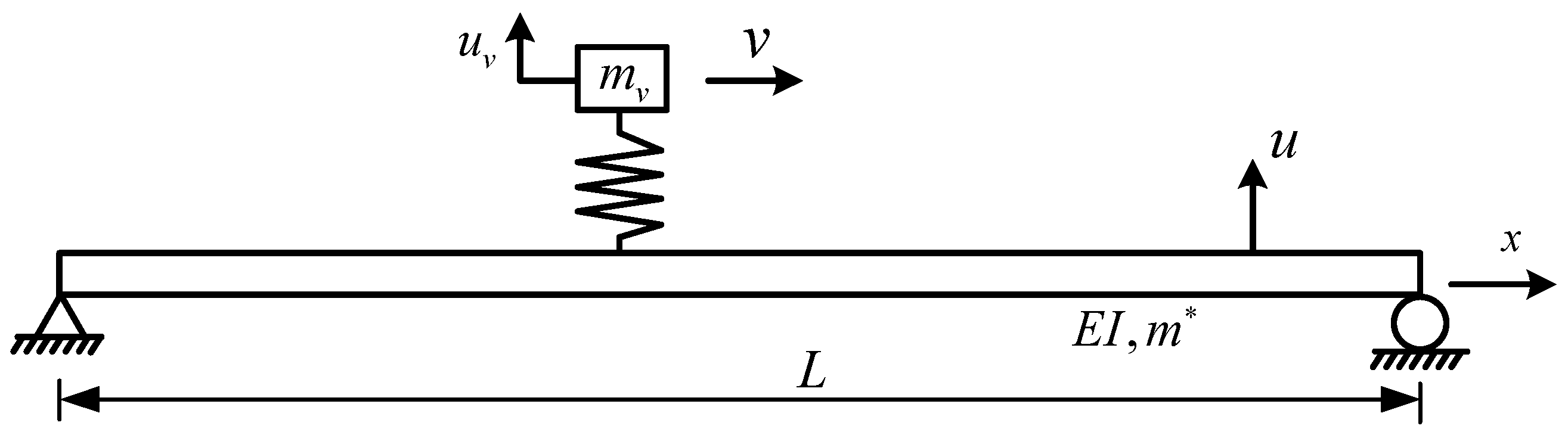
2. Theoretical Background and Formulations
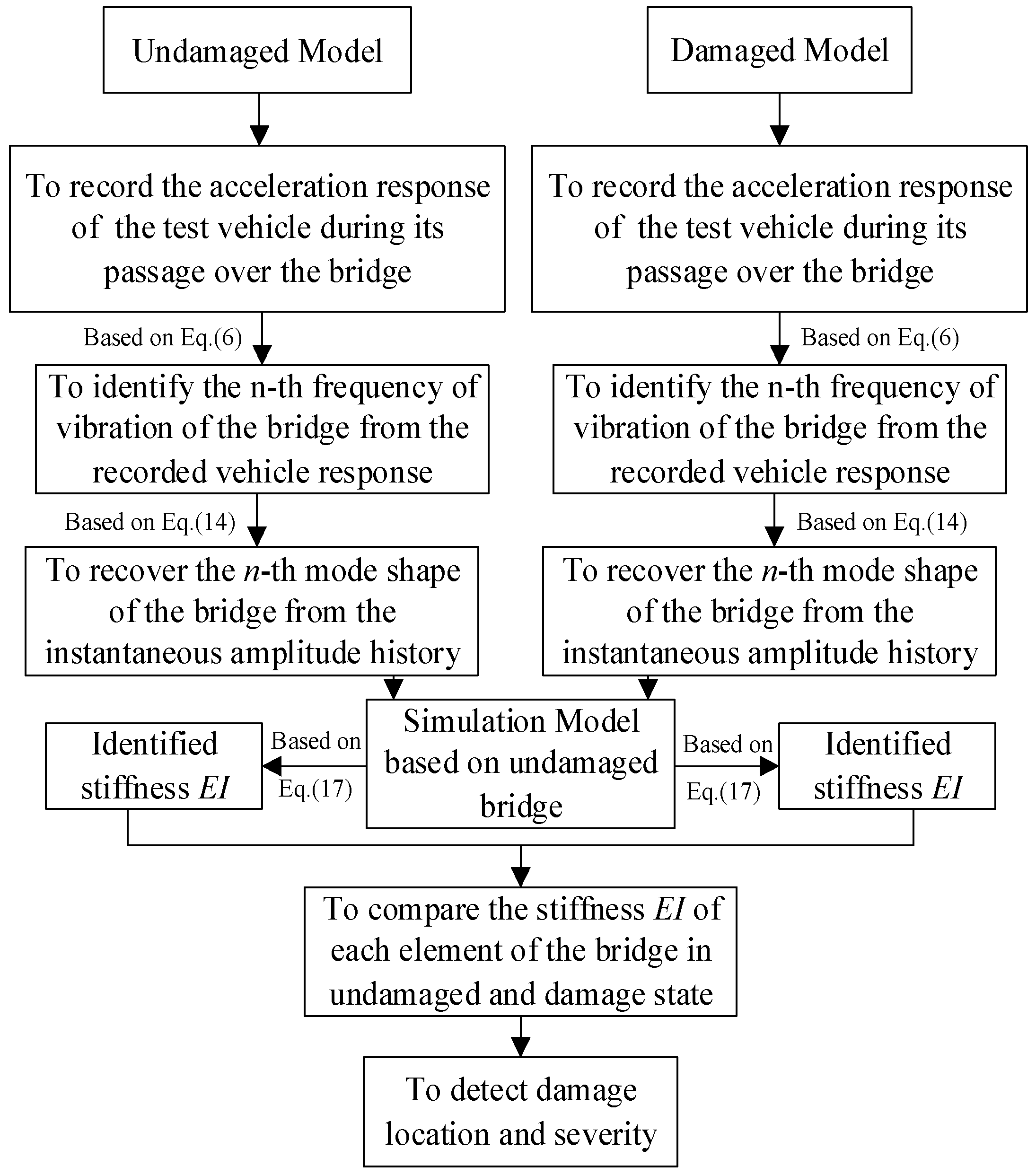
2.1. Frequency Domain Method
- (1)
- It is assumed that a previous monitoring of the bridge of concern has been completed using the procedure stated below, which is regarded as the undamaged state.
- (2)
- The acceleration response is recorded for the test vehicle during its passage over the bridge for the current monitoring, which is suspected as the damaged state.
- (3)
- Identify the n-th frequency of vibration of the bridge from the recorded vehicle response in the previous and current runs of monitoring.
- (4)
- Recover the n-th mode shape of the bridge from the instantaneous amplitude of the component response corresponding to the n-th frequency.
- (5)
- Calculate the stiffness EI using the n-th frequency and corresponding mode shape for the bridge, based on which the structural damage is detected.
- (6)
- If no damage is detected, then the current monitoring is regarded as the undamaged state, and the same procedure of damage detection is repeated for the next monitoring.
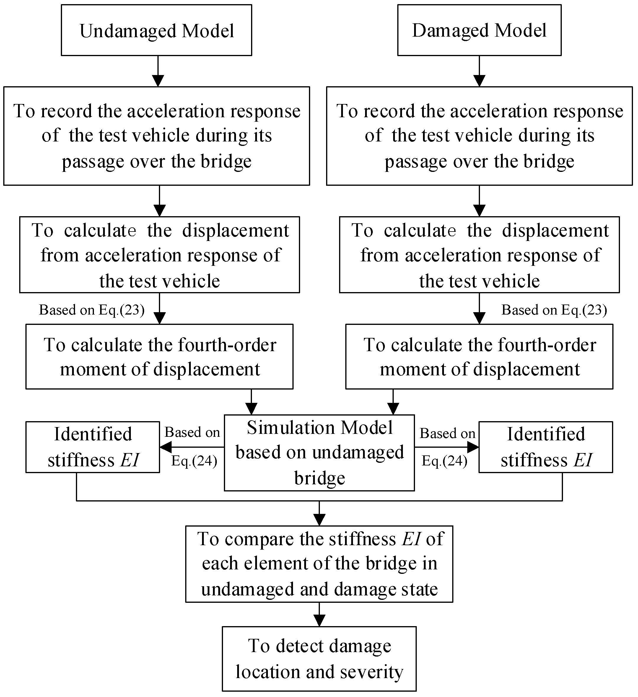
2.2. Time-Domain Method
- (1)
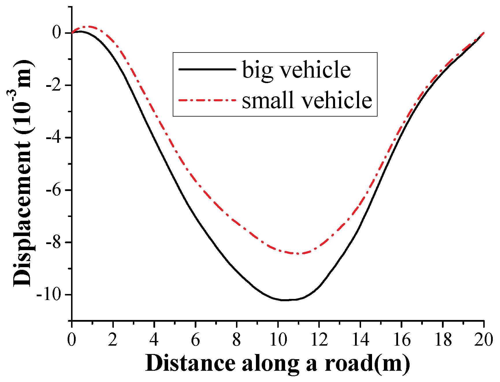
- Measure the displacement responses of the test vehicle, or calculate the displacement from the acceleration response of the test vehicle during its passage over the bridge for the undamaged and damaged states.
- (2)
- The actual statistical moments of the measured displacement responses of the test vehicle with the undamaged and damaged states, , are estimated using Equation (23).
- (3)
- Given the vector that collects all of the stiffness parameters for all of the elements representing the bridge FE model using initial values based on the calculated stiffness, e.g., from the frequency-domain method, the theoretical statistical moments of the displacement responses of the test vehicle, , are calculated based on the FE model of the bridge and also making use of Equation (23).
- (4)
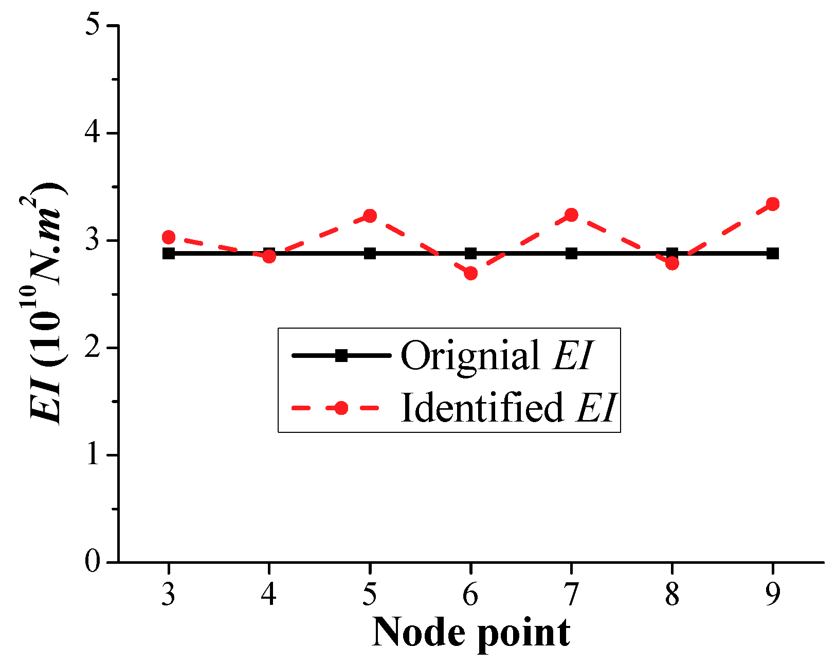
- Substituting and into Equation (24), the vector collecting the structural stiffness values of all of the elements of the FE model of the bridge can be identified by the constrained nonlinear least-squares method for the undamaged and damaged states.
- (5)
- All of the attributes of the structural damage of the bridge, including the existence, location, and severity, can be detected by comparing the identified vector of the stiffness values of the undamaged bridge, , to that of the damaged bridge, .
3. Parameters of the Test Vehicle Numerical Study
4. Considered Scenarios in the Numerical Study
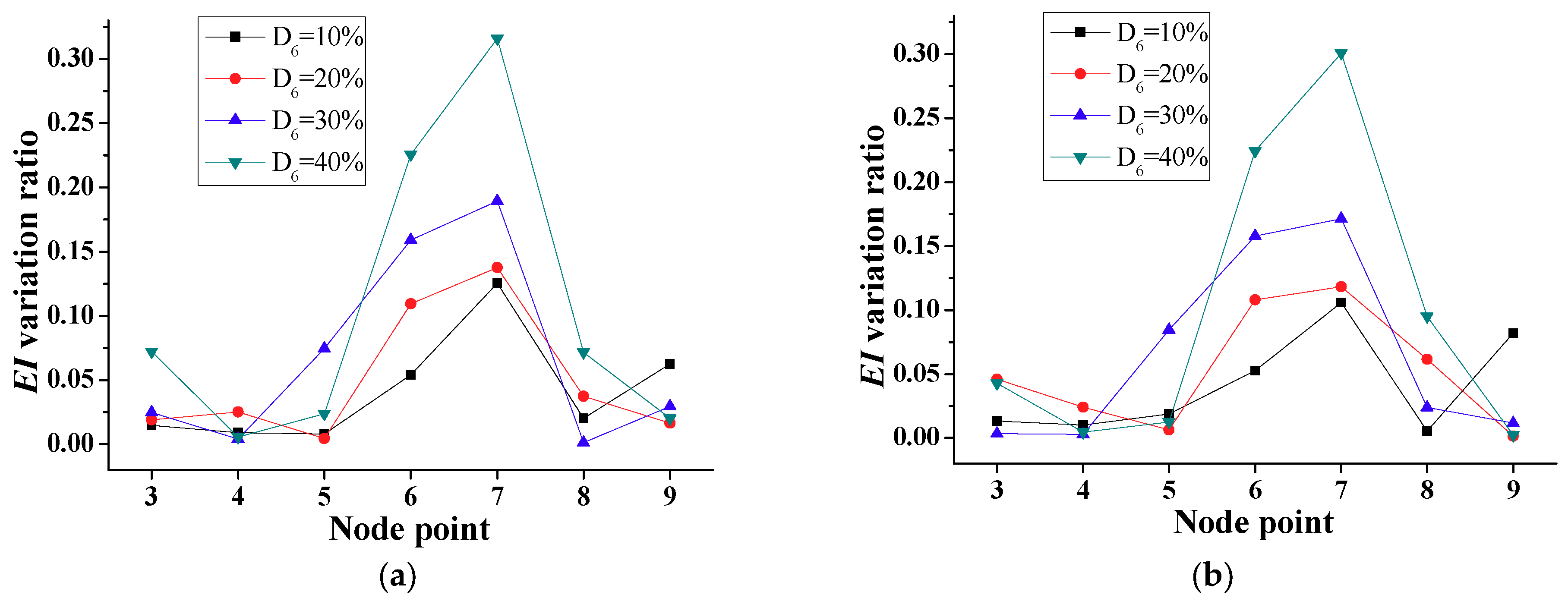
4.1. Frequency-Domain Method
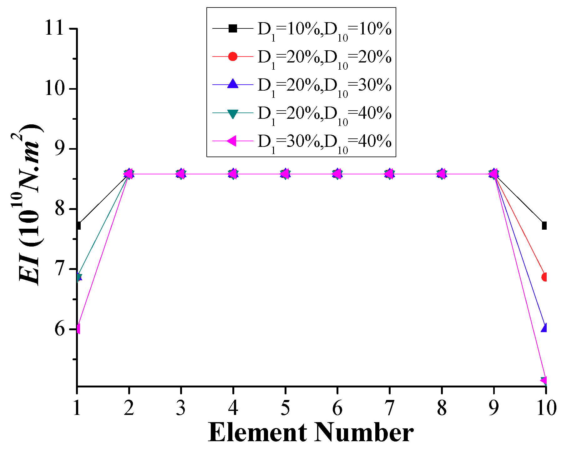
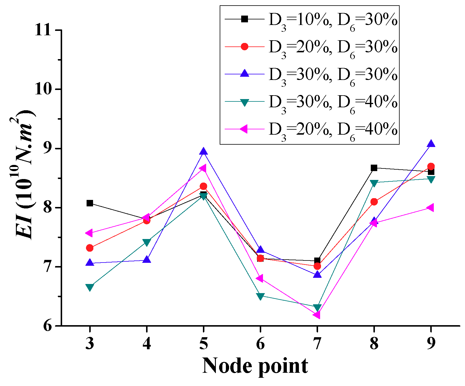
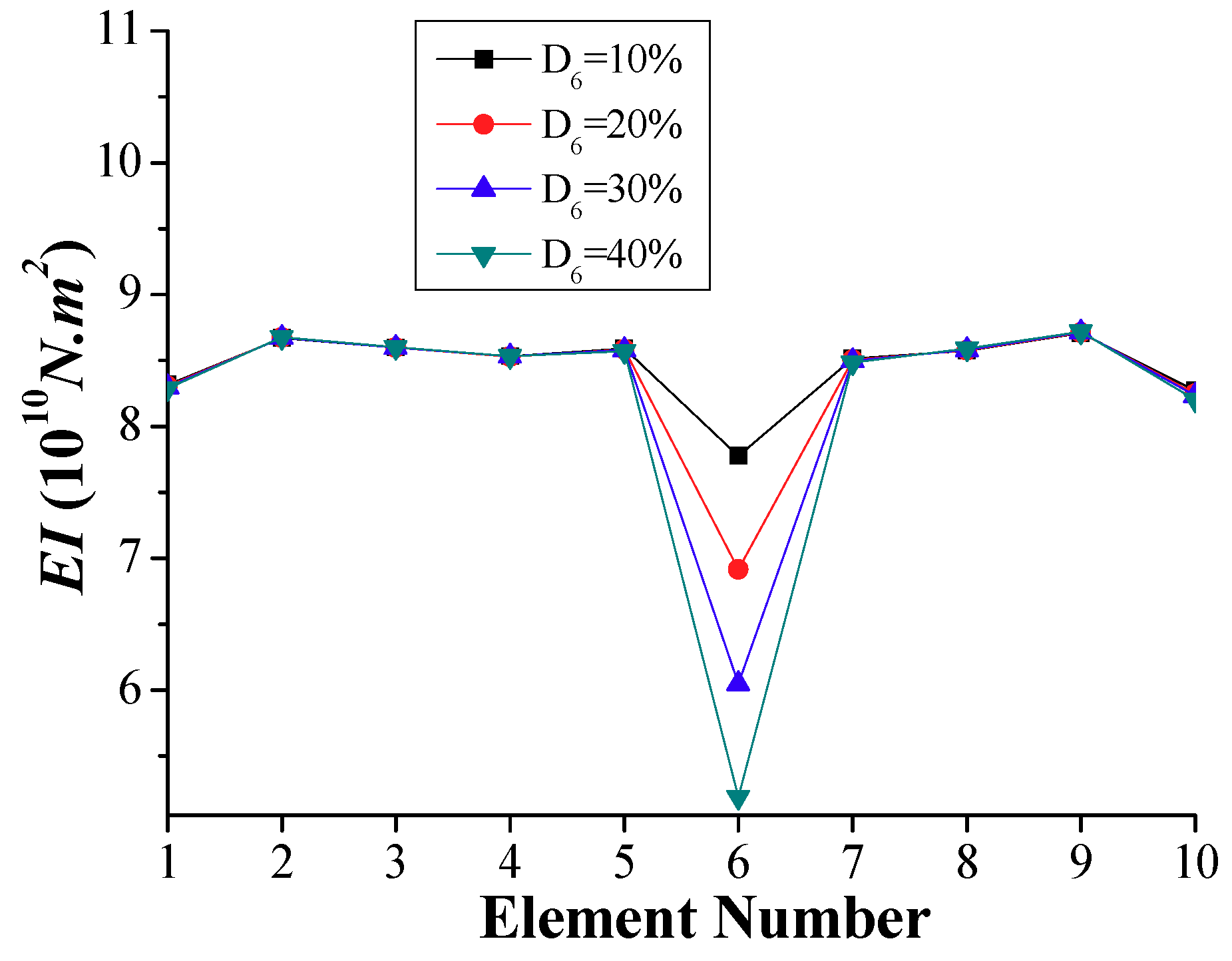
4.2. Time-Domain Method
5. Measurement Error Study
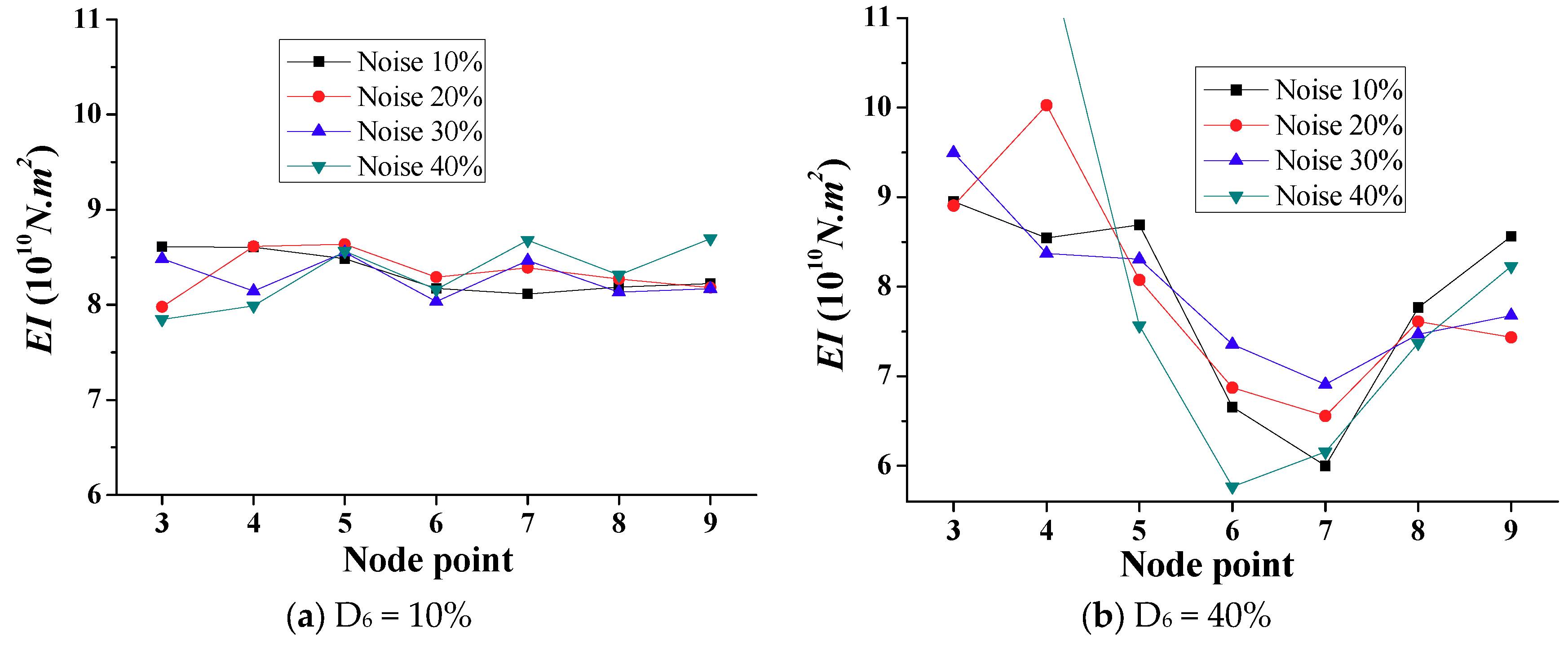
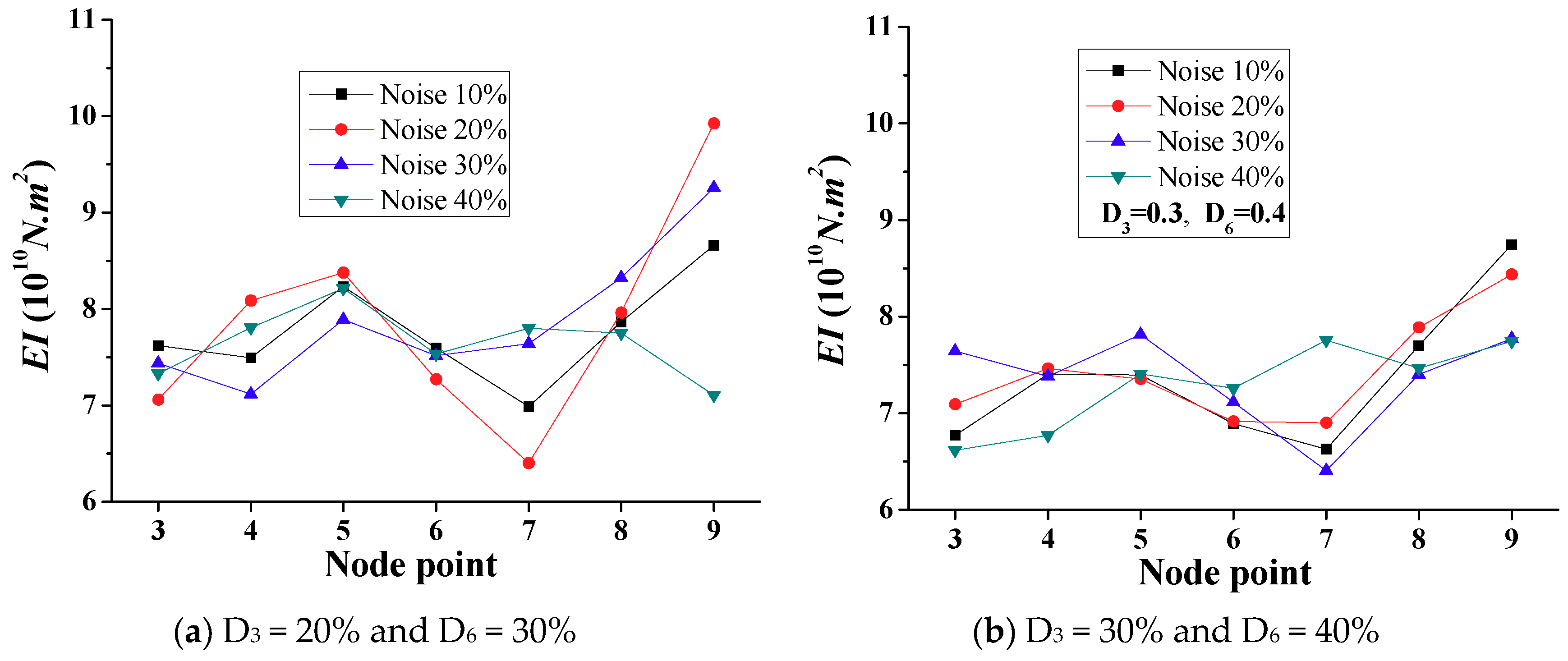
5.1. Considering Noise in the Frequency-Domain Method
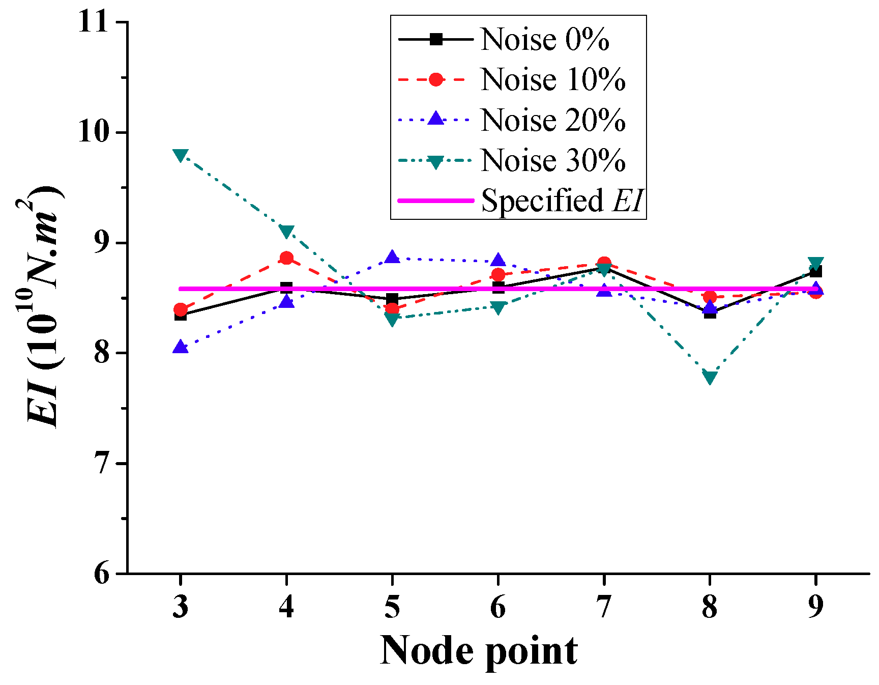
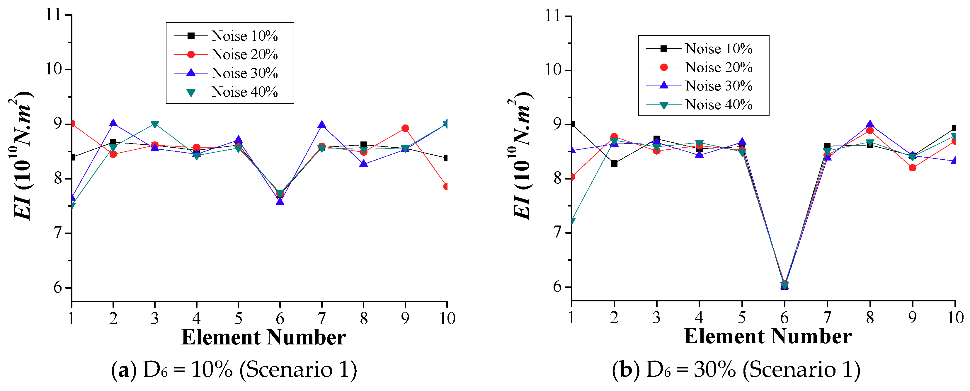
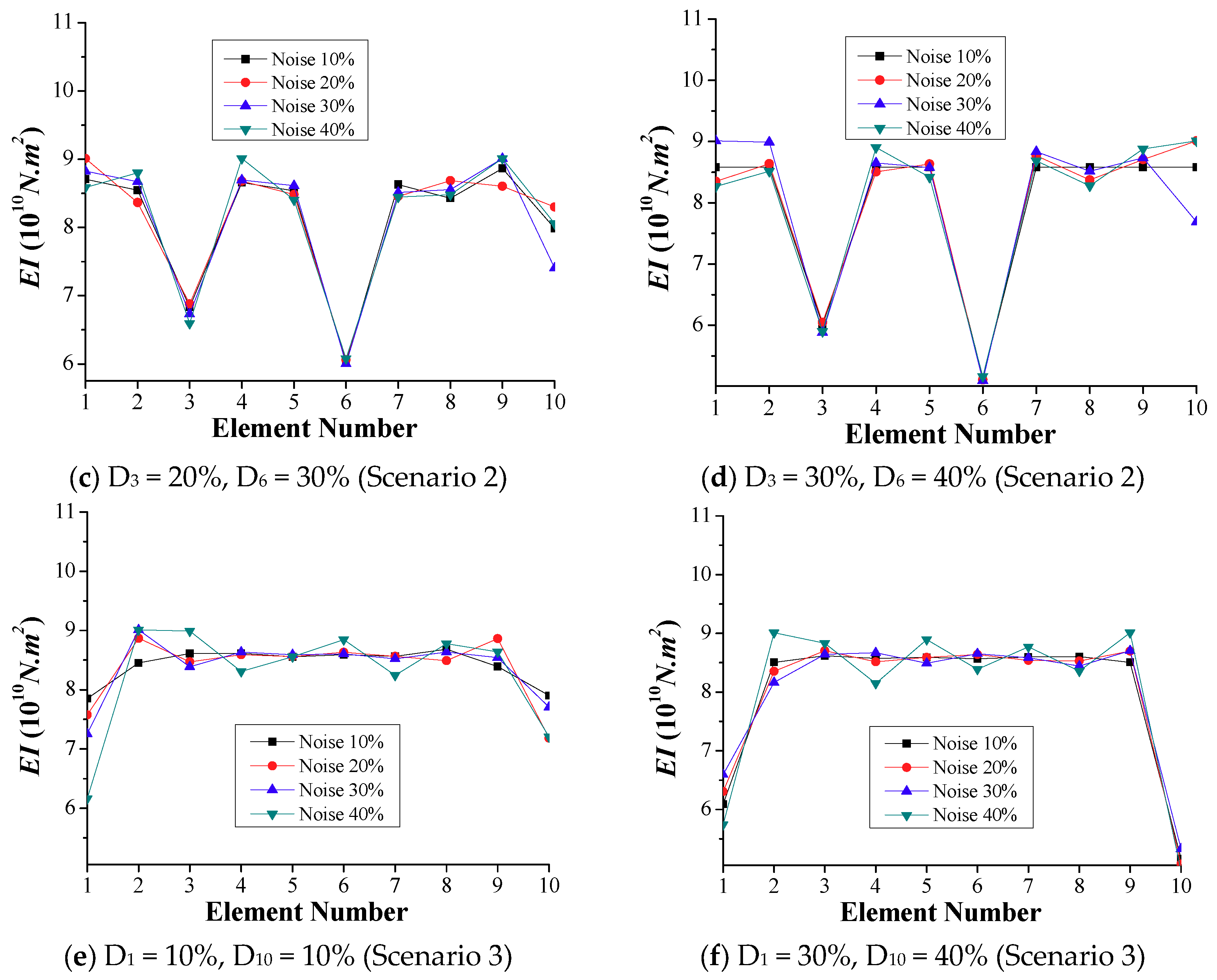
5.2. Considering Noise in the Time-Domain Method
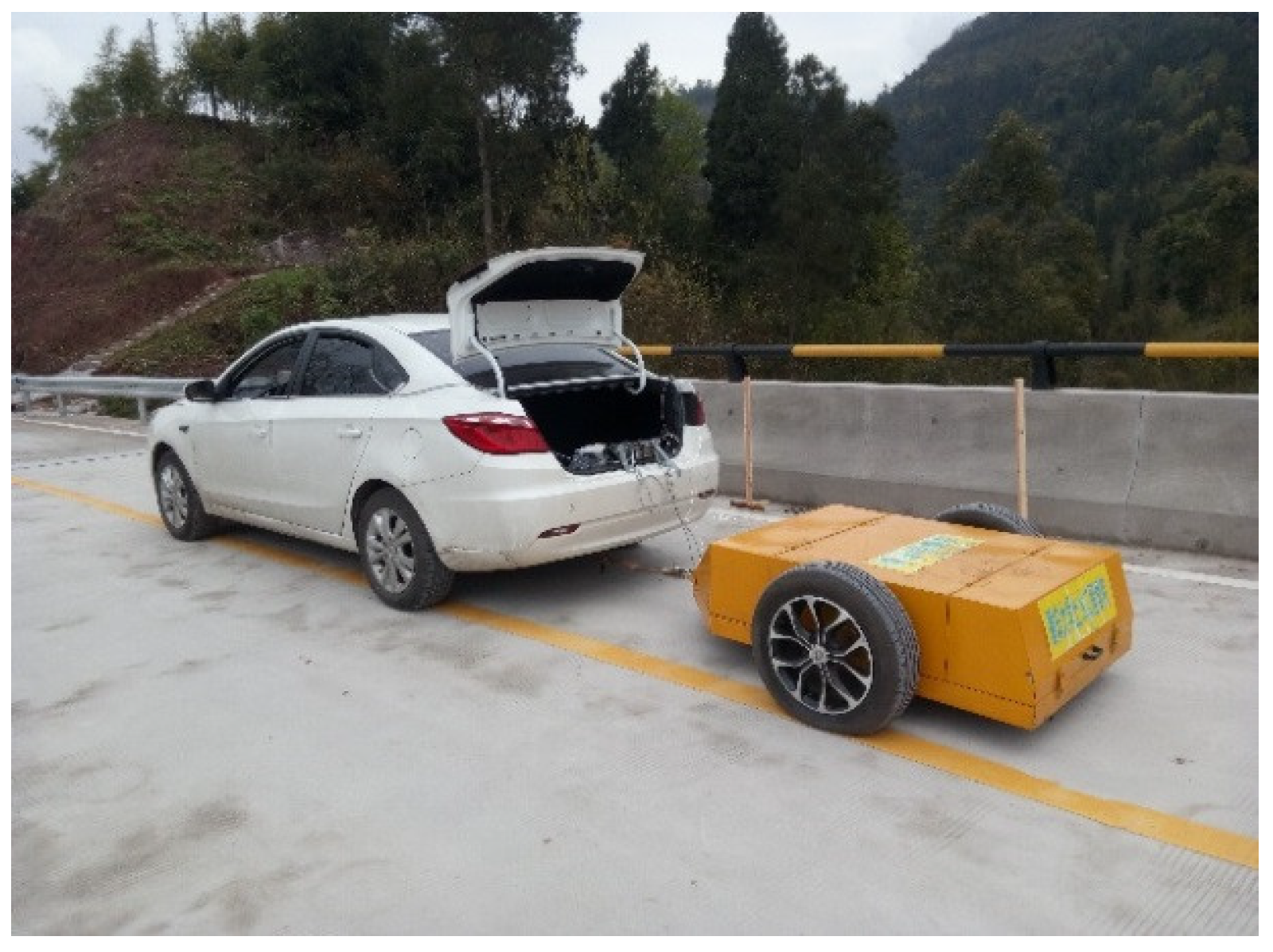
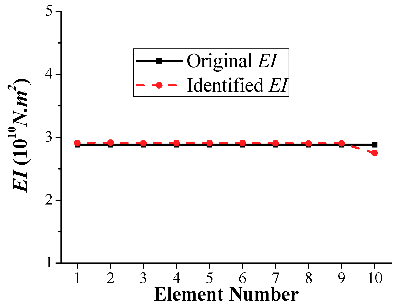
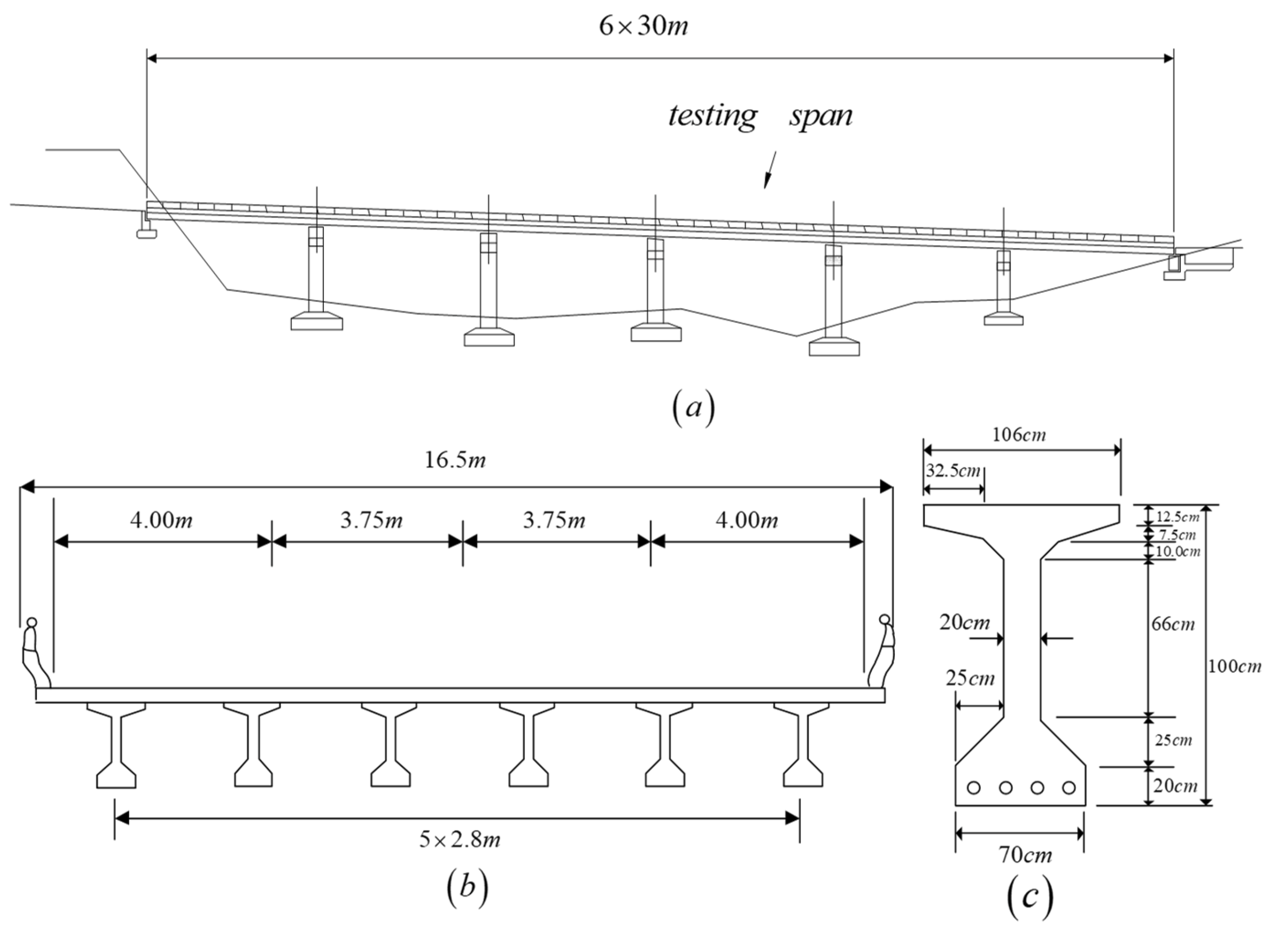
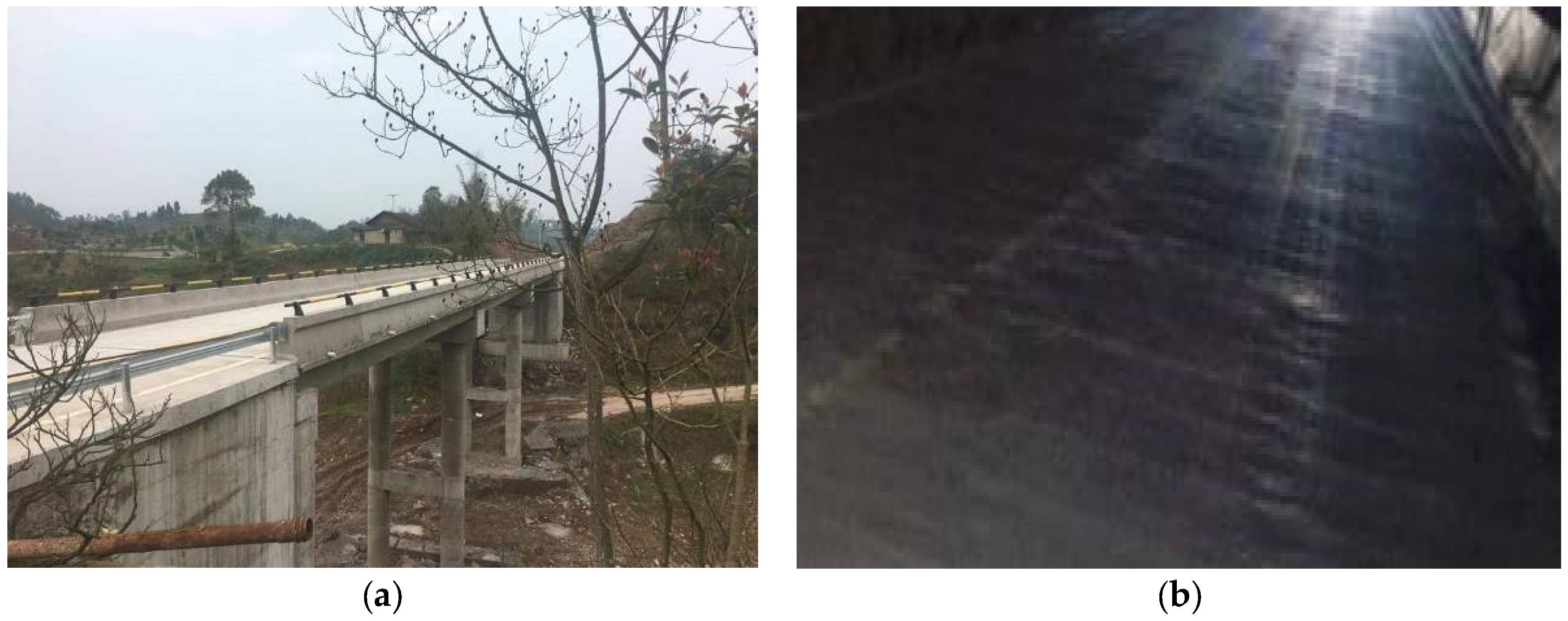
6. Field Test Study
7. Results Discussion
8. Conclusions
- The proposed indirect approach, including the frequency-domain and time-domain methods, requires no parametric inputs, which is more general compared to other structural damage identification, e.g., wavelet-based methods. Therefore, the proposed approach can be directly adopted for the structural damage identification of in-service bridge structures without additional and cumbersome calibration.
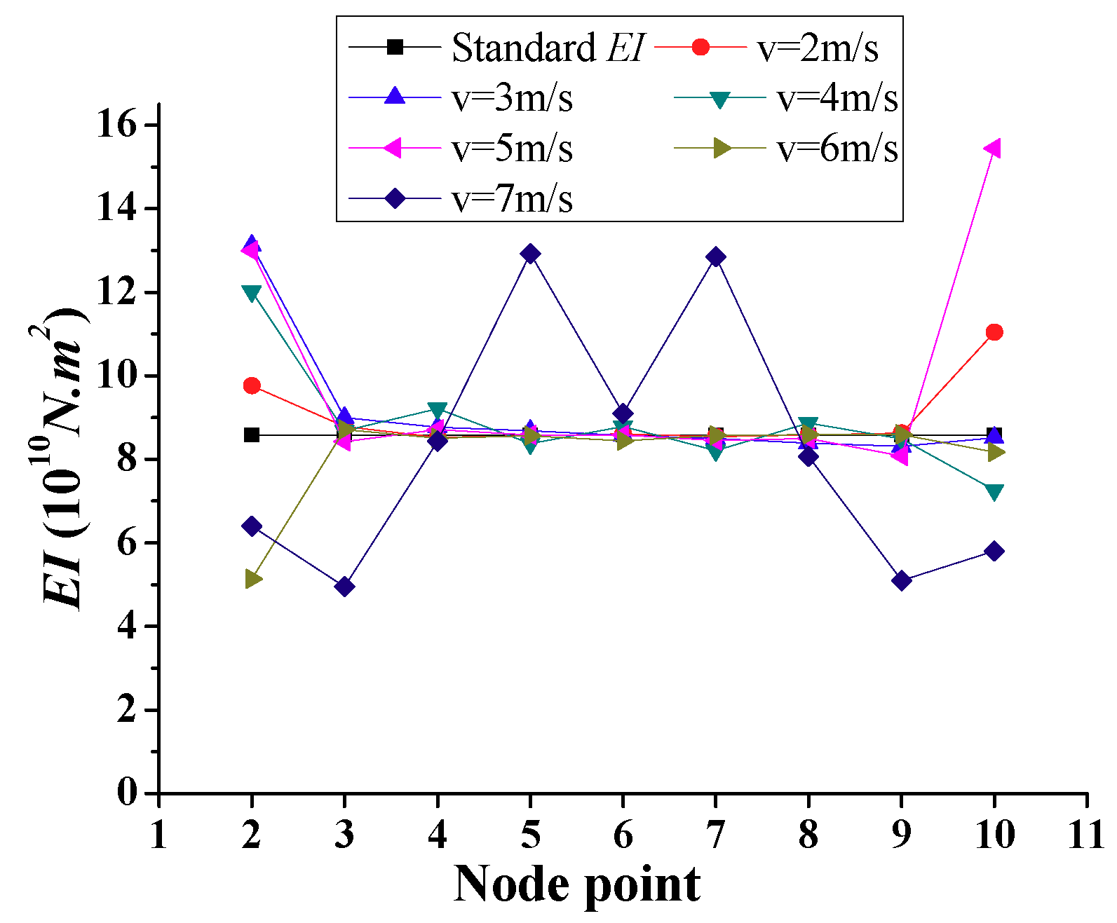
- The frequency-domain method is advantageous with its high cost efficiency, since it can estimate the initial stiffness of the bridge based on the first mode of vibration, and is sufficient for identifying damage location(s) apart from the end regions of the bridge. However, this method requires that the speed of the passing vehicle should be lower than 6 m/s during the measurement, and it is not applicable for damage identification in the boundary nodes.
- Although the time-domain method is computationally intensive due to the additional optimization steps, it has the advantages of high accuracy, reliability, and robustness, and is feasible for use especially in the end regions of the bridge, which is suitable for identifying damage location(s) and damage severities.
- The field test study shows that the identified results errors from using the frequency-domain method and time-domain method are below 16% and 5% respectively; this indicates that the two methods are useful for assessment bending stiffness with a practical bridge. Moreover, it indicated that the time-domain method is advantageous with higher accuracy, robustness, and reliability as compared to the frequency-domain method.
- In the practical assessment of the bridge health conditions, the frequency-domain approach is suitable in the preliminary phase to estimate the initial damage conditions of the bridge on site. Subsequently, in the final phase of the investigation, the time-domain approach can provide more detailed and comprehensive results with high accuracy and reliability.
Author Contributions
Funding
Conflicts of Interest
References
- Hou, L.Q.; Zhao, X.F.; Ou, J.P.; Liu, C.C. A Review of Nondeterministic Methods for Structural Damage Diagnosis. J. Vib. Shock 2014, 33, 50–58. [Google Scholar]
- Amezquita-Sanchez, J.P.; Adele, H. Signal Processing Techniques for Vibration-Based Health Monitoring of Smart Structures. Arch. Comput. Methods Eng. 2016, 23, 1–15. [Google Scholar] [CrossRef]
- Maeck, J. Damage Assessment of Civil Engineering Structure by Vibration Monitoring. Ph.D. Thesis, Department of Civil Engineering, Katholieke Universiteit Leuven, Leuven, Belgium, 2003. [Google Scholar]
- Huth, O.; Feltrin, G.; Maeck, J.; Kilic, N.; Motavalli, M. Damage Identification Using Modal Data: Experiences on a Prestressed Concrete Bridge. ASCE J. Struct. Eng. 2005, 131, 1898–1910. [Google Scholar] [CrossRef]
- Xu, Y.L.; Zhang, J.; Li, J.C. Experimental Investigation on Statistical Moment-Based Structural Damage Detection Method. J. Struct. Health Monit. 2009, 8, 555–571. [Google Scholar] [CrossRef]
- Xu, Y.L.; Zhang, J.; Li, J.; Wang, X.M. Stochastic Damage Detection Method for Building Structures with Parametric Uncertainties. J. Sound Vib. 2011, 330, 4725–4737. [Google Scholar] [CrossRef]
- Li, W.M.; Jiang, Z.H.; Wang, T.L.; Zhu, H.P. Optimization Method Based on Generalized Pattern Search Algorithm to Identify Bridge Parameters Indirectly by a Passing Vehicle. J. Sound Vib. 2014, 333, 364–380. [Google Scholar] [CrossRef]
- Yang, Y.; Mosalam, K.M.; Liu, H.; Huang, X.N. An Improved Direct Stiffness Calculation Method for Damage Detection of Beam Structures. Struct. Control Health Monit. 2013, 20, 835–851. [Google Scholar] [CrossRef]
- Yang, Y.; Mosalam, K.M.; Liu, G.; Wang, X.L. Damage Detection Using Improved Direct Stiffness Calculations-A Case Study. Int. J. Struct. Stab. Dyn. 2016, 16, 1640002. [Google Scholar] [CrossRef]
- Yang, Y.; Yang, Y.B.; Chen, Z.X. Seismic Damage Assessment of RC Structures under Shaking Table Tests Using The Modified Direct Stiffness Calculation Method. Eng. Struct. 2017, 131, 574–585. [Google Scholar] [CrossRef]
- Blachowski, B.; An, Y.H.; Spencer, B.F.; Ou, J.P. Axial Strain Accelerations Approach for Damage Localization in Statically Determinate Truss Structures. Comput.-Aided Civ. Infrastruct. Eng. 2017, 32, 304–314. [Google Scholar] [CrossRef]
- Kim, C.W.; Chang, K.C.; Kitauchi, S.; McGetrick, P.J. A Field Experiment on a Steel Gerber-truss Bridge for Damage Detection Utilizing Vehicle-induced Vibrations. Struct. Health Monit. 2016, 15, 421–429. [Google Scholar] [CrossRef]
- Sevillano, E.; Sun, R.; Perera, R. Damage Evaluation of Structures with Uncertain Parameters via Interval Analysis and FE Model Updating Methods. Struct. Control Health Monit. 2016, 24, 1–22. [Google Scholar] [CrossRef]
- Yang, Y.; Li, J.L.; Zhou, C.H.; Law, S.S.; Lv, L. Damage Detection of Structures with Parametric Uncertainties Based on Fusion of Statistical Moments. J. Sound Vib. 2018. [Google Scholar] [CrossRef]
- Mao, J.X.; Wang, H.; Feng, D.M.; Tao, T.Y.; Zheng, W.Z. Investigation of Dynamic Properties of Long-span Cable-stayed Bridges based on One-year Monitoring Data under Normal Operating Condition. Struct. Control Health Monit. 2018, 25, 1–19. [Google Scholar] [CrossRef]
- Wang, H.; Mao, J.X.; Huang, J.H.; Li, A.Q. Modal Identification of Sutong Cable-Stayed Bridge during Typhoon Haikui Using Wavelet Transform Method. J. Perform. Constr. Facil. 2016, 30, 04016001-1-11. [Google Scholar] [CrossRef]
- Yang, Y.B.; Lin, C.W.; Yan, J.D. Extracting Bridge Frequencies from the Dynamic Response of a Passing Vehicle. J. Sound Vib. 2004, 272, 471–493. [Google Scholar] [CrossRef]
- Yang, Y.B.; Lin, C.W. Vehicle-Bridge Interaction Dynamics and Potential Applications. J. Sound Vib. 2005, 284, 205–226. [Google Scholar] [CrossRef]
- Yang, Y.B.; Lin, C.W. Use of a Passing Vehicle to Scan the Fundamental Bridge Frequencies: An Experimental Verification. Eng. Struct. 2005, 27, 1865–1878. [Google Scholar]
- Yang, Y.B.; Chang, K.C. Extraction of Bridge Frequencies from the Dynamic Response of a Passing Vehicle Enhanced by the EMD Technique. J. Sound Vib. 2009, 322, 718–739. [Google Scholar] [CrossRef]
- Feng, D.M.; Feng, M.Q. Output-Only Damage Detection Using Vehicle-induced Displacement Response and Mode Shape Curvature Index. Struct. Control Health Monit. 2016, 23, 1088–1107. [Google Scholar] [CrossRef]
- Obrien, E.J.; Keenahan, J. Drive-by Damage Detection in Bridges Using the Apparent Profile. Struct. Control Health Monit. 2015, 22, 813–825. [Google Scholar] [CrossRef]
- Behroozinia, P.; Khaleghian, S.; Taheri, S.; Mirzaeifar, R. Damage Diagnosis in Intelligent Tires Using Time-domain and Frequency-domain Analysis. Mech. Based Des. Struct. Mach. 2018. [Google Scholar] [CrossRef]
- McGetrick, P.J.; Gonazalez, A.; O’Brien, E.J. Theoretical Investigation of the Use of a Moving Vehicle to Identify Bridge Dynamic Parameters. Non-Destruct. Test. Cond. Monit. 2009, 51, 433–438. [Google Scholar] [CrossRef]
- Yang, Y.B.; Li, Y.C.; Chang, K.C. Constructing the Mode Shapes of a Bridge from a Passing Vehicle: A Theoretical Study. Smart Struct. Syst. 2014, 13, 797–819. [Google Scholar] [CrossRef]
- Vujanovic, B. Conservation Laws of Dynamical Systems via D’Alembert’s Principle. Int. J. Non-Linear Mech. 1978, 13, 185–197. [Google Scholar] [CrossRef]
- Clough, R.W.; Penzien, J. Dynamics of Structures; McGraw-Hill: New York, NY, USA, 1993. [Google Scholar]
- Bu, J.Q.; Law, S.S.; Zhu, X.Q. Innovative Bridge Condition Assessment from Dynamic Response of a Passing Vehicle. ASCE J. Eng. Mech. 2006, 132, 1372–1379. [Google Scholar] [CrossRef]
- Xiang, Z.H.; Dai, X.W.; Zhang, Y.; Lu, Q.H. The Tap-Scan Method for Damage Detection of Bridge Structures. Interact. Multiscale Mech. 2010, 3, 173–191. [Google Scholar] [CrossRef]
- Kiureghian, A.D. Non-ergodicity and PEER’s framework formula. Earthq. Eng. Struct. Dyn. 2005, 34, 1643–1652. [Google Scholar] [CrossRef]


| Scenario | Group | Damaged Element(s) | Reduction in Element Stiffness (%) | ||||
|---|---|---|---|---|---|---|---|
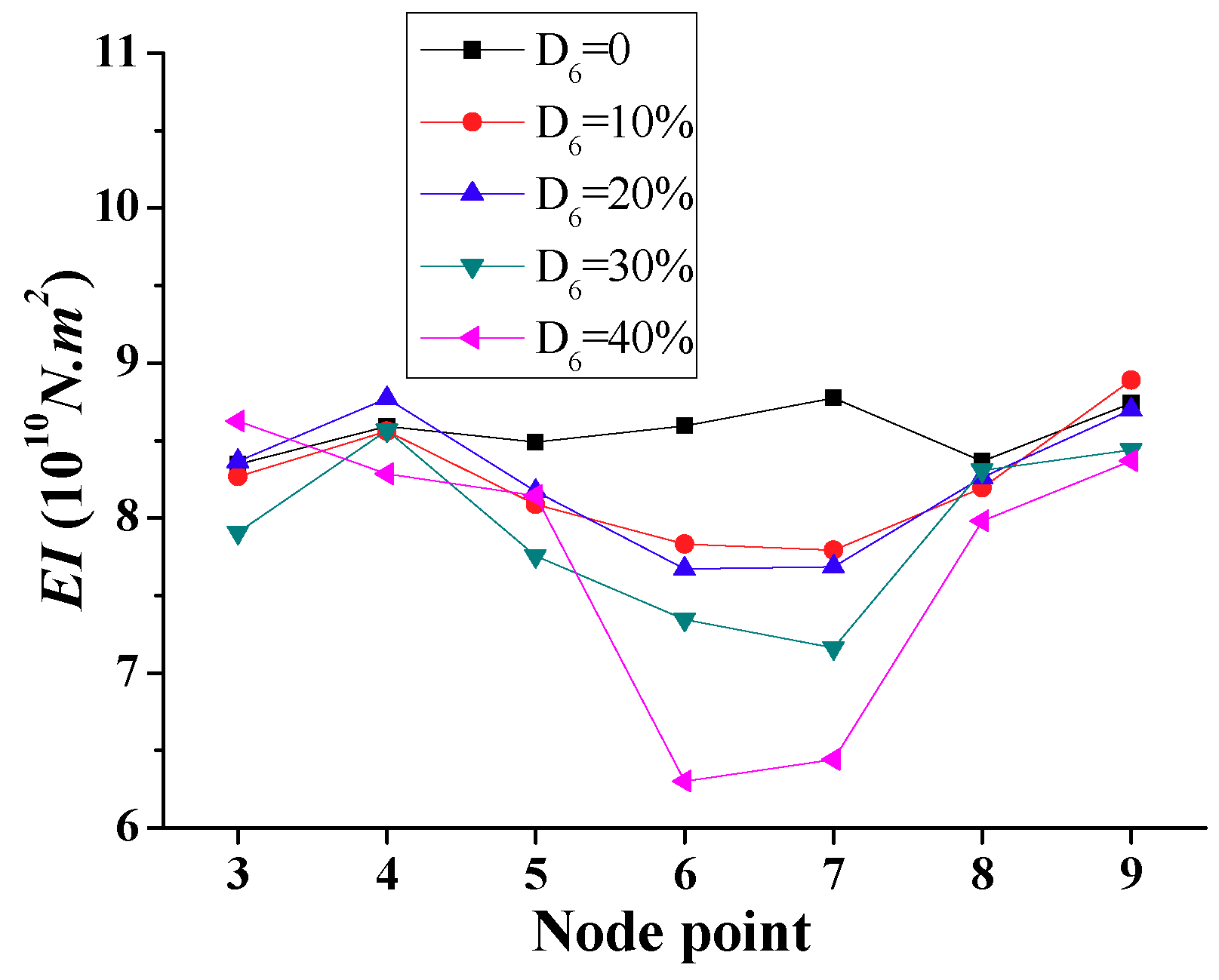
| 1 | D6 | 6 | D6 = 0 | D6 = 10 | D6 = 20 | D6 = 30 | D6 = 40 |
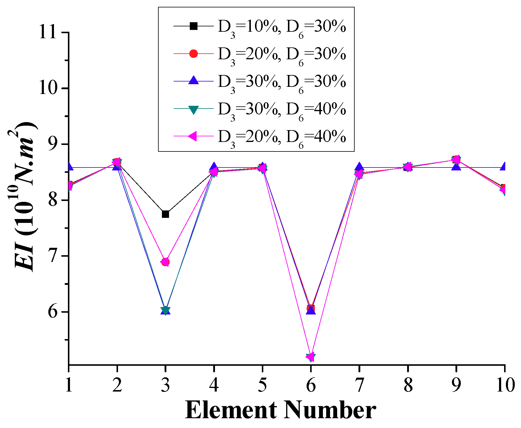
| 2 | D3, D6 | 3 & 6 | D3 = 10 D6 = 30 | D3 = 20 D6 = 30 | D3 = 30 D6 = 30 | D3 = 30 D6 = 40 | D3 = 20 D6 = 40 |
| 3 | D1, D10 | 1 & 10 | D1 = 10 D10 = 10 | D3 = 20 D6 = 20 | D3 = 20 D6 = 30 | D3 = 20 D6 = 40 | D3 = 30 D6 = 40 |
© 2018 by the authors. Licensee MDPI, Basel, Switzerland. This article is an open access article distributed under the terms and conditions of the Creative Commons Attribution (CC BY) license (http://creativecommons.org/licenses/by/4.0/).
Share and Cite
Yang, Y.; Zhu, Y.; Wang, L.L.; Jia, B.Y.; Jin, R. Structural Damage Identification of Bridges from Passing Test Vehicles. Sensors 2018, 18, 4035. https://doi.org/10.3390/s18114035
Yang Y, Zhu Y, Wang LL, Jia BY, Jin R. Structural Damage Identification of Bridges from Passing Test Vehicles. Sensors. 2018; 18(11):4035. https://doi.org/10.3390/s18114035
Chicago/Turabian StyleYang, Yang, Yuanhao Zhu, Li Lei Wang, Bao Yulong Jia, and Ruoyu Jin. 2018. "Structural Damage Identification of Bridges from Passing Test Vehicles" Sensors 18, no. 11: 4035. https://doi.org/10.3390/s18114035
APA StyleYang, Y., Zhu, Y., Wang, L. L., Jia, B. Y., & Jin, R. (2018). Structural Damage Identification of Bridges from Passing Test Vehicles. Sensors, 18(11), 4035. https://doi.org/10.3390/s18114035