2D LiDAR SLAM Back-End Optimization with Control Network Constraint for Mobile Mapping

Abstract
:1. Introduction
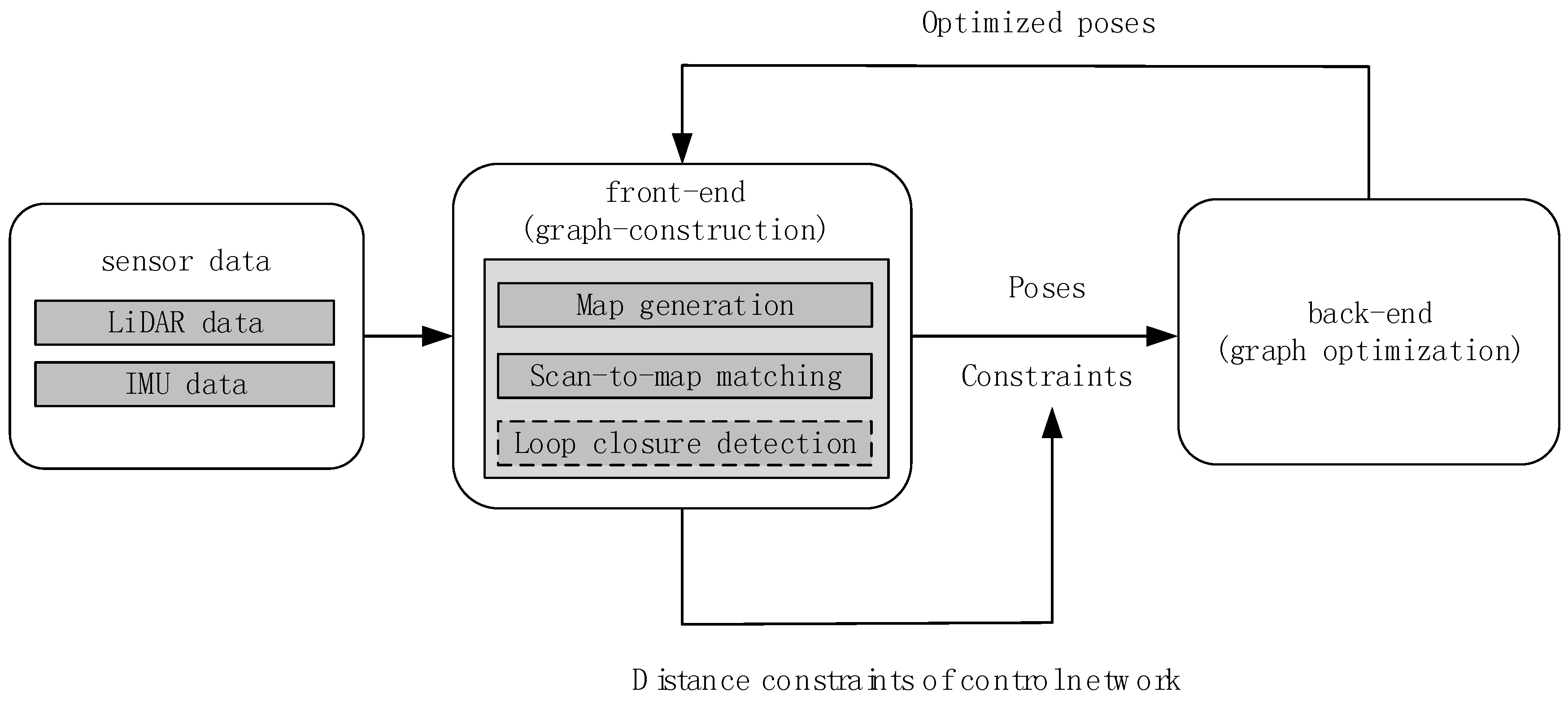
2. System Overview
3. Method
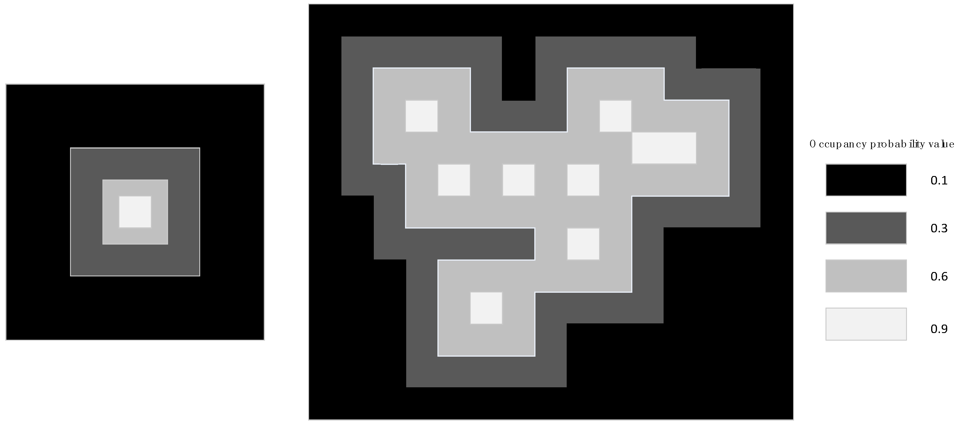
3.1. Multiresolution Map Generation
3.2. Front-End Scan-to-Map Matching
3.3. Back-End Optimization
3.4. Back-End Optimization with Distance Constraints of Control Network
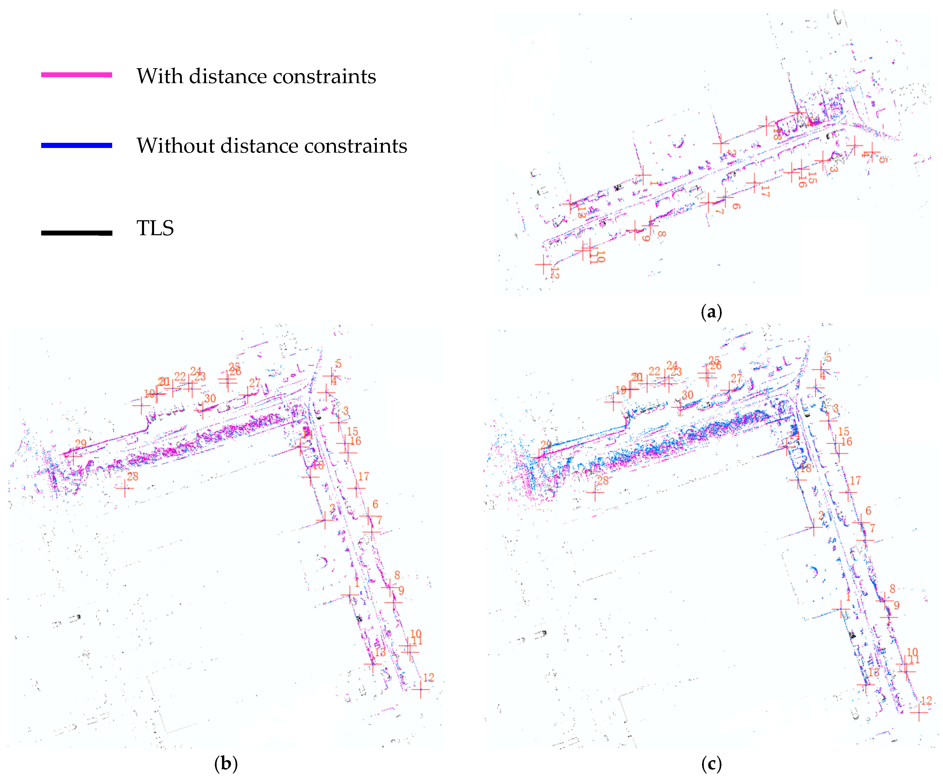
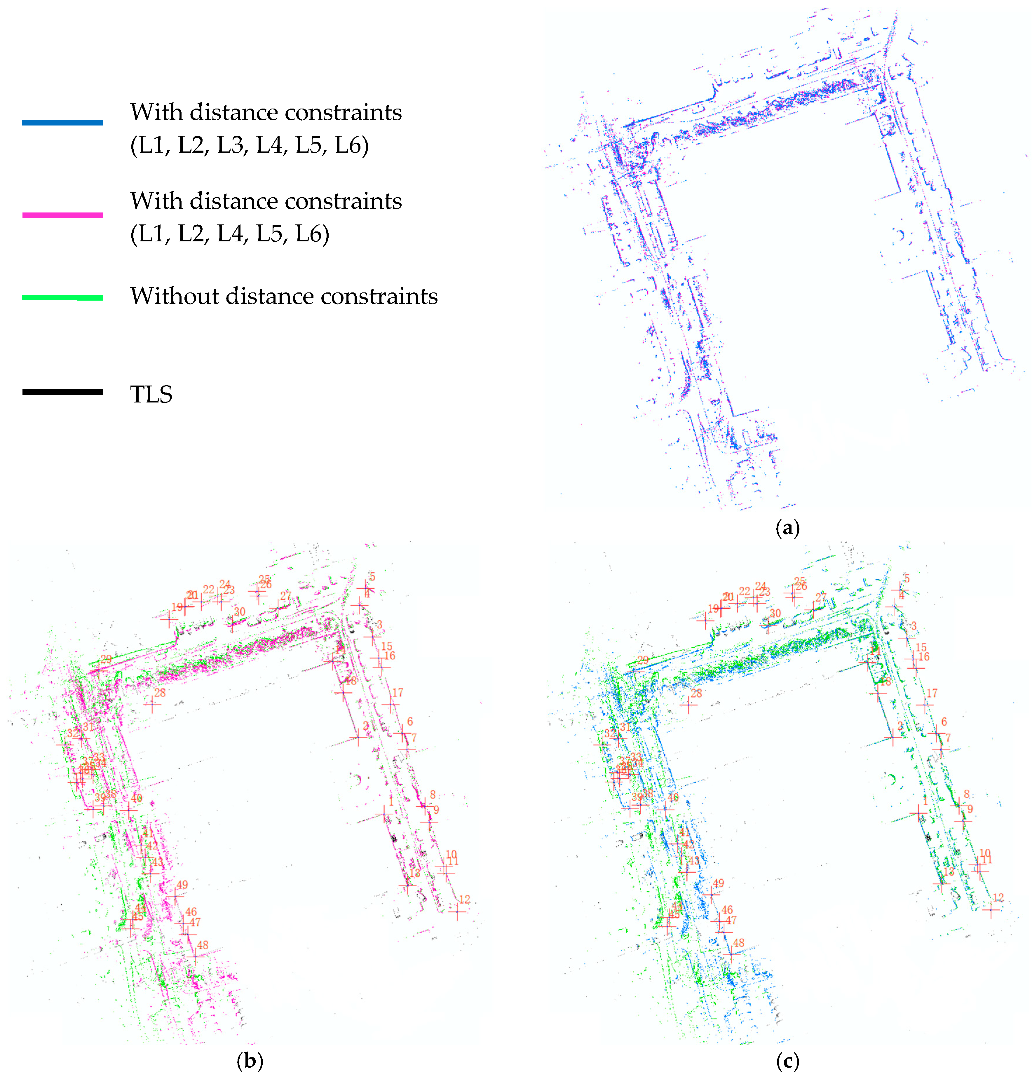
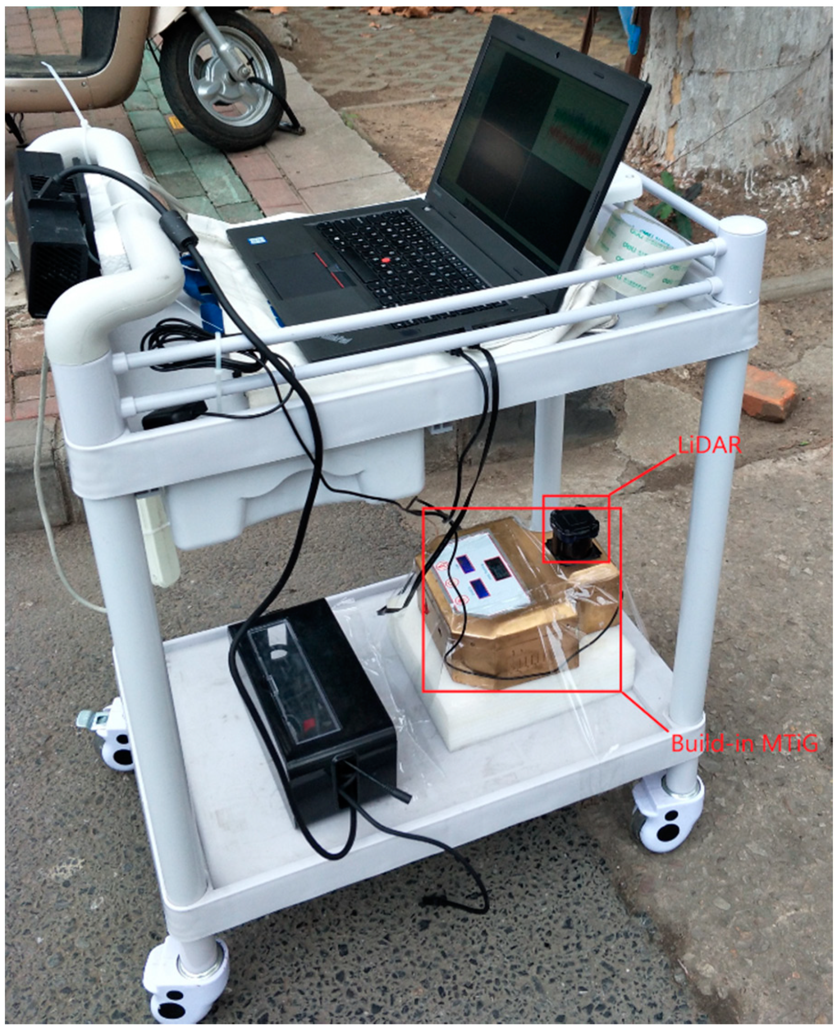
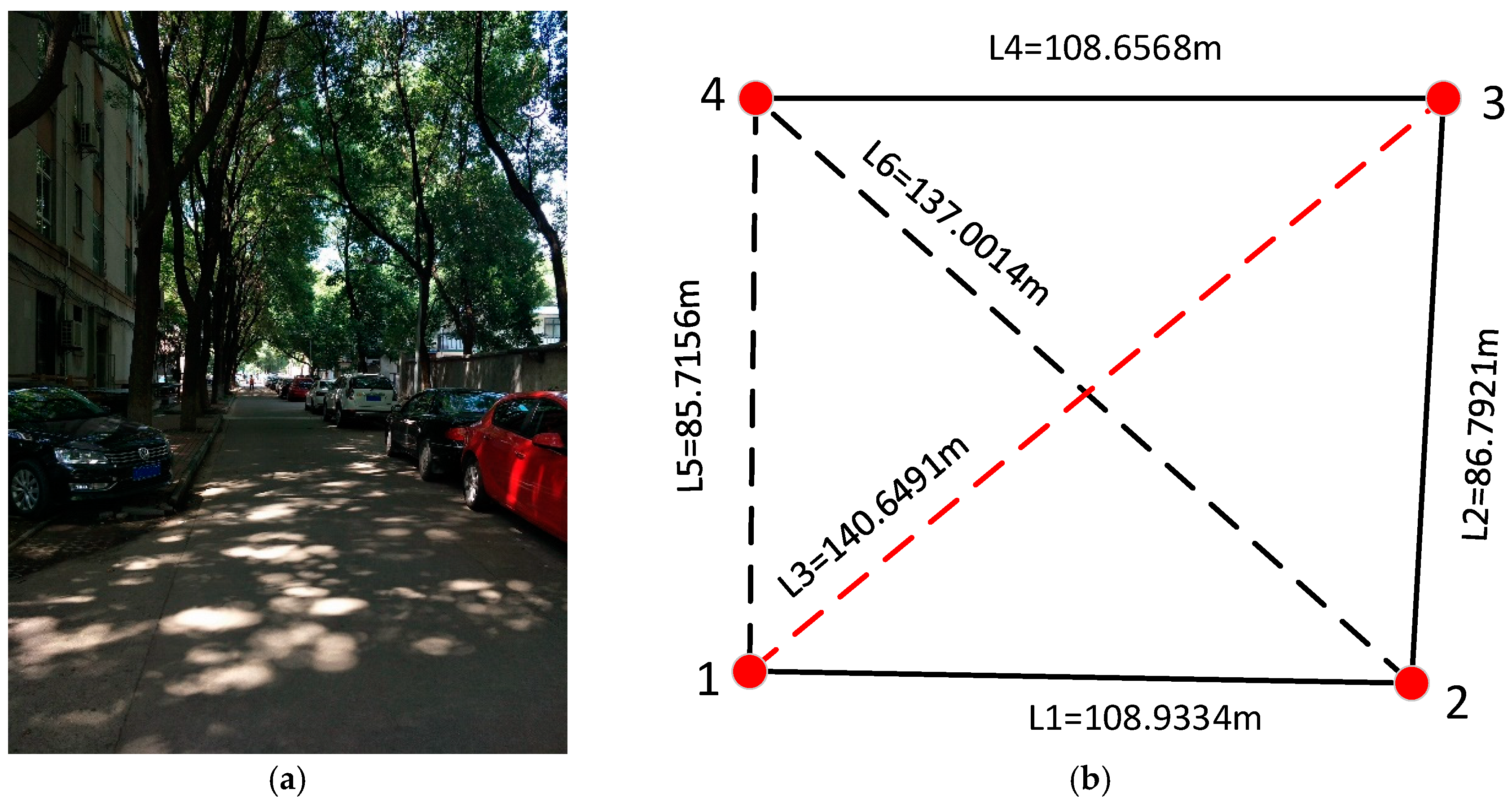
4. Field Test and Results
5. Conclusions
Author Contributions
Funding
Conflicts of Interest
References
- Bailey, T.; Durrant-Whyte, H. Simultaneous localization and mapping (SLAM): Part II. IEEE Robot. Autom. Mag. 2006, 13, 108–117. [Google Scholar] [CrossRef]
- Hartley, R.; Zisserman, A. Multiple View Geometry in Computer Vision; Cambridge University Press: Cambridge, UK, 2000; pp. 1865–1872. [Google Scholar]
- Thrun, S.; Burgard, W.; Fox, D. Probabilistic Robotics; MIT Press: Cambridge, MA, USA, 2005. [Google Scholar]
- Xie, X.; Yu, Y.; Lin, X.; Sun, C. An EKF SLAM algorithm for mobile robot with sensor bias estimation. In Proceedings of the 2017 32nd Youth Academic Annual Conference of Chinese Association of Automation, Hefei, China, 19–21 May 2017; pp. 281–285. [Google Scholar]
- Zhang, T.; Wu, K.; Song, J.; Huang, S.; Dissanayake, G. Convergence and Consistency Analysis for A 3D Invariant-EKF SLAM. IEEE Robot. Autom. Lett. 2017, 2, 733–740. [Google Scholar] [CrossRef]
- Huang, S.; Dissanayake, G. Convergence and Consistency Analysis for Extended Kalman Filter Based SLAM. IEEE Trans. Robot. 2007, 23, 1036–1049. [Google Scholar] [CrossRef] [Green Version]
- Thrun, S.; Leonard, J.J. Simultaneous Localization and Mapping. IEEE Trans. Intell. Transp. Syst. 2015, 13, 541–552. [Google Scholar]
- Yatim, N.M.; Buniyamin, N. Particle filter in simultaneous localization and mapping (Slam) using differential drive mobile robot. J. Teknol. 2015, 77, 91–97. [Google Scholar]
- Montemerlo, M.S. Fastslam: A Factored Solution to the Simultaneous Localization and Mapping Problem with Unknown Data Association. Ph.D. Thesis, Carnegie Mellon University, Pittsburgh, PA, USA, 2003. [Google Scholar]
- Grisetti, G.; Kummerle, R.; Stachniss, C.; Burgard, W. A tutorial on graph-based SLAM. IEEE Intell. Transp. Syst. Mag. 2010, 2, 31–43. [Google Scholar] [CrossRef]
- Thrun, S. Simultaneous localization and mapping. In Robotics and Cognitive Approaches to Spatial Mapping; Springer: Berlin/Heidelberg, Germany, 2007; pp. 13–41. [Google Scholar]
- Li, J.; Zhan, H.; Chen, B.M.; Reid, I.; Lee, G.H. Deep learning for 2D scan matching and loop closure. In Proceedings of the 2017 IEEE/RSJ International Conference on Intelligent Robots and Systems (IROS), Vancouver, BC, Canada, 24–28 September 2017; pp. 763–768. [Google Scholar]
- Labbé, M.; Michaud, F. Online global loop closure detection for large-scale multi-session graph-based SLAM. In Proceedings of the 2014 IEEE/RSJ International Conference on Intelligent Robots and Systems, Chicago, IL, USA, 14–18 September 2014; pp. 2661–2666. [Google Scholar]
- Magnusson, M.; Andreasson, H.; Nuchter, A.; Lilienthal, A.J. Appearance-based loop detection from 3D laser data using the normal distributions transform. J. Field Robot. 2010, 26, 892–914. [Google Scholar] [CrossRef]
- Bosse, M.; Zlot, R. Keypoint design and evaluation for place recognition in 2D lidar maps. Robot. Auton. Syst. 2009, 57, 1211–1224. [Google Scholar] [CrossRef] [Green Version]
- Tipaldi, G.D.; Spinello, L.; Burgard, W. Geometrical FLIRT phrases for large scale place recognition in 2D range data. In Proceedings of the 2013 IEEE International Conference on Robotics and Automation, Karlsruhe, Germany, 6–10 May 2013; pp. 2693–2698. [Google Scholar]
- Himstedt, M.; Frost, J.; Hellbach, S.; Böhme, H.-J.; Maehle, E. Large scale place recognition in 2D LIDAR scans using Geometrical Landmark Relations. In Proceedings of the 2014 IEEE/RSJ International Conference on Intelligent Robots and Systems, Chicago, IL, USA, 14–18 September 2014; pp. 5030–5035. [Google Scholar]
- Callmer, J.; Ramos, F.; Nieto, J. Learning to detect loop closure from range data. In Proceedings of the IEEE International Conference on Robotics and Automation, Kobe, Japan, 12–17 May 2009; pp. 1990–1997. [Google Scholar]
- Hess, W.; Kohler, D.; Rapp, H.; Andor, D. Real-time loop closure in 2D LIDAR SLAM. In Proceedings of the IEEE International Conference on Robotics and Automation, Stockholm, Sweden, 16–21 May 2016; pp. 1271–1278. [Google Scholar]
- Qian, C.; Liu, H.; Tang, J.; Chen, Y.; Kaartinen, H.; Kukko, A.; Zhu, L.; Liang, X.; Chen, L.; Hyyppä, J. An Integrated GNSS/INS/LiDAR-SLAM Positioning Method for Highly Accurate Forest Stem Mapping. Remote Sens. 2016, 9, 3. [Google Scholar] [CrossRef]
- Hening, S.; Ippolito, C.A.; Krishnakumar, K.S.; Stepanyan, V.; Teodorescu, M. 3D LiDAR SLAM Integration with GPS/INS for UAVs in Urban GPS-Degraded Environments. In Proceedings of the AIAA Information Systems-AIAA Infotech @ Aerospace, Grapevine, TX, USA, 9–13 January 2017. [Google Scholar]
- Kümmerle, R.; Steder, B.; Dornhege, C.; Kleiner, A.; Grisetti, G.; Burgard, W. Large scale graph-based SLAM using aerial images as prior information. Auton. Robot. 2011, 30, 25–39. [Google Scholar] [CrossRef]
- Schuster, F.; Keller, C.G.; Rapp, M.; Haueis, M.; Curio, C. Landmark based radar SLAM using graph optimization. In Proceedings of the IEEE International Conference on Intelligent Transportation Systems, Rio de Janeiro, Brazil, 1–4 November 2016; pp. 2559–2564. [Google Scholar]
- Homm, F.; Kaempchen, N.; Ota, J.; Burschka, D. Efficient occupancy grid computation on the GPU with lidar and radar for road boundary detection. In Proceedings of the 2010 IEEE Intelligent Vehicles Symposium, San Diego, CA, USA, 21–24 June 2010; pp. 1006–1013. [Google Scholar]
- Tang, J.; Chen, Y.; Jaakkola, A.; Liu, J.; Hyyppä, J.; Hyyppä, H. NAVIS-An UGV indoor positioning system using laser scan matching for large-area real-time applications. Sensors 2014, 14, 11805–11824. [Google Scholar] [CrossRef] [PubMed]
- Besl, P.J.; Mckay, N.D. Method for registration of 3-D shapes. IEEE Trans. Pattern Anal. Mach. Intell. 1992, 14, 239–256. [Google Scholar] [CrossRef]
- Censi, A. An ICP variant using a point-to-line metric. In Proceedings of the 2008 IEEE International Conference on Robotics and Automation, Pasadena, CA, USA, 19–23 May 2008; pp. 19–25. [Google Scholar]
- Bosse, M.C. Atlas: A Framework for Large Scale Automated Mapping and Localization; Massachusetts Institute of Technology: Cambridge, MA, USA, 2004. [Google Scholar]
- Kohlbrecher, S.; Stryk, O.V.; Meyer, J.; Klingauf, U. A flexible and scalable SLAM system with full 3D motion estimation. In Proceedings of the IEEE International Symposium on Safety, Security, and Rescue Robotics, Kyoto, Japan, 1–5 November 2011; pp. 155–160. [Google Scholar]
- Clausen, J. Branch and Bound Algorithms—Principles and Examples. Parallel Process. Lett. 1999, 22, 658–663. [Google Scholar]


| LiDAR | IMU | ||
|---|---|---|---|
| Product model | Hokuyo UTM-EX | Product model | MEMS-level MTi-G |
| Sampling frequency | 10 Hz | Sample frequency | 200 Hz |
| Scan range | 0.1–30 m | Gyroscope bias | 200°/h |
| Scan angle | 270° | Accelerometer | 2000 mGal (1 Gal = 1 cm/s2) |
| Angular resolution | 0.25° | ||
| Total Station | Product model | ||
| Product model | TIANYU CST-632 | Product model | FARO Focus3D X130 HDR |
| Angle Accuracy | 2 s | Range Accuracy | ±2 mm |
| Range Accuracy | ±(2 + 2 × 10⁻⁶ * D) mm | Scan range | 0.6–130 m |
| Number of Constraints | Track Length | Number of Common Feature Points | RMS (without Constraint) | RMS (with Constraint) |
|---|---|---|---|---|
| 1 (L1) | 108.9 m | 18 | 0.1904 m | 0.1612 m |
| 2 (L1, L2) | 195.6 m | 30 | 0.7303 m | 0.6608 m |
| 3 (L1, L2, L3) | 195.6 m | 30 | 0.7303 m | 0.2369 m |
| Number of Constraints | Track Length | Number of Common Feature Points | RMS (without Constraint) | RMS (with Constraint) |
|---|---|---|---|---|
| 6 (L1, L2, L3, L4, L5, L6) | 304.3 m | 49 | 1.6462 m | 0.3356 m |
| 5 (L1, L2, L4, L5, L6) | 304.3 m | 49 | 1.6462 m | 0.3614 m |
© 2018 by the authors. Licensee MDPI, Basel, Switzerland. This article is an open access article distributed under the terms and conditions of the Creative Commons Attribution (CC BY) license (http://creativecommons.org/licenses/by/4.0/).
Share and Cite
Wen, J.; Qian, C.; Tang, J.; Liu, H.; Ye, W.; Fan, X. 2D LiDAR SLAM Back-End Optimization with Control Network Constraint for Mobile Mapping. Sensors 2018, 18, 3668. https://doi.org/10.3390/s18113668
Wen J, Qian C, Tang J, Liu H, Ye W, Fan X. 2D LiDAR SLAM Back-End Optimization with Control Network Constraint for Mobile Mapping. Sensors. 2018; 18(11):3668. https://doi.org/10.3390/s18113668
Chicago/Turabian StyleWen, Jingren, Chuang Qian, Jian Tang, Hui Liu, Wenfang Ye, and Xiaoyun Fan. 2018. "2D LiDAR SLAM Back-End Optimization with Control Network Constraint for Mobile Mapping" Sensors 18, no. 11: 3668. https://doi.org/10.3390/s18113668
APA StyleWen, J., Qian, C., Tang, J., Liu, H., Ye, W., & Fan, X. (2018). 2D LiDAR SLAM Back-End Optimization with Control Network Constraint for Mobile Mapping. Sensors, 18(11), 3668. https://doi.org/10.3390/s18113668