A New Algorithm for High-Integrity Detection and Compensation of Dual-Frequency Cycle Slip under Severe Ionospheric Storm Conditions

Abstract
1. Introduction
2. Cycle-Slip Detection and Compensation Algorithm
2.1. Dual-Frequency Cycle-Slip Detection Method
2.1.1. TDSD Carrier-Phase Observations
2.1.2. Receiver Clock Drift Estimate
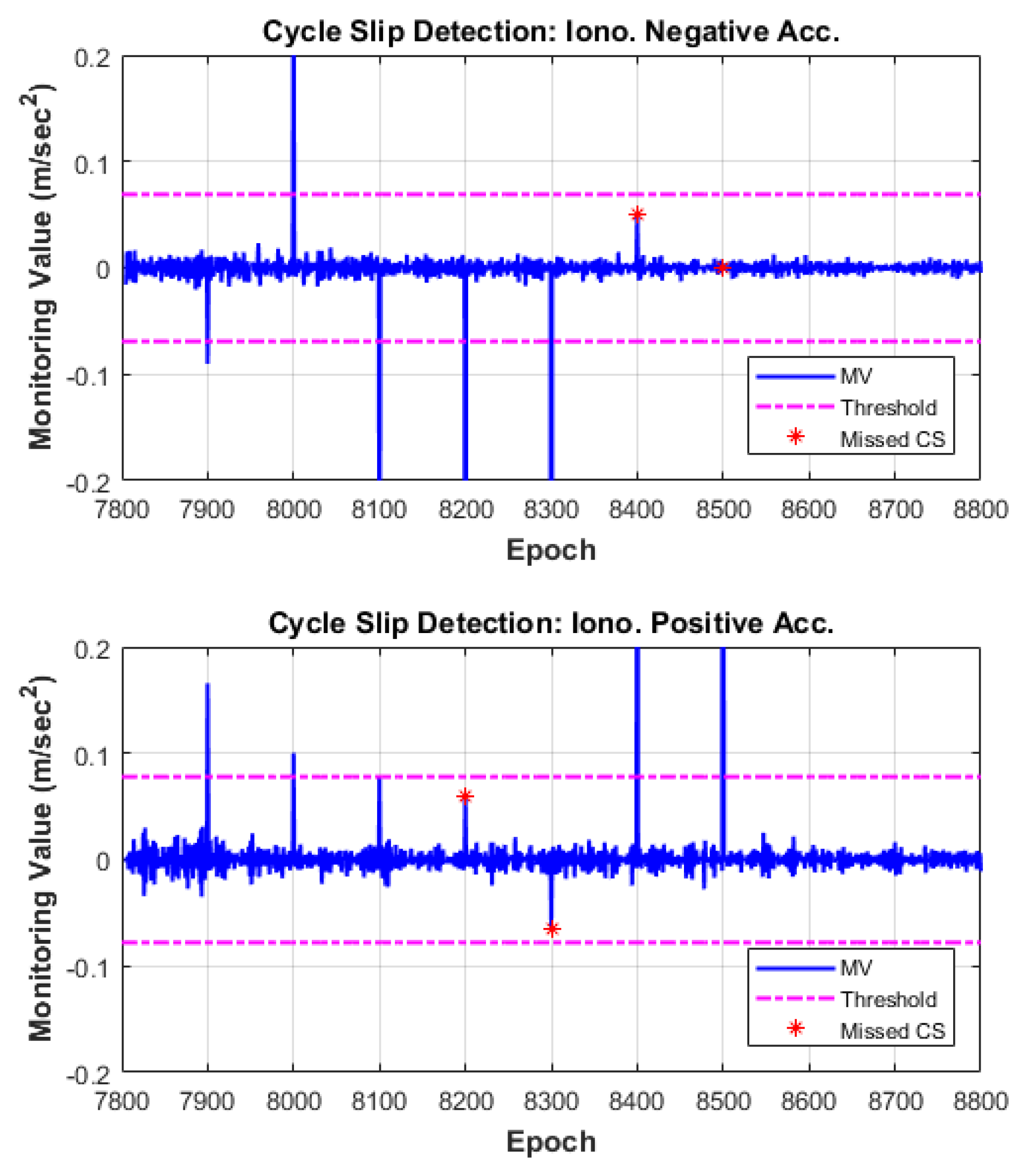
2.1.3. Cycle-Slip Detection Using the Ionospheric Acceleration
2.2. Error Propagation in Monitoring Values
2.2.1. Theoretical Noise Analysis of Monitoring Values
2.2.2. Actual Error Distribution of Monitoring Values
2.3. Threshold Determination Scheme
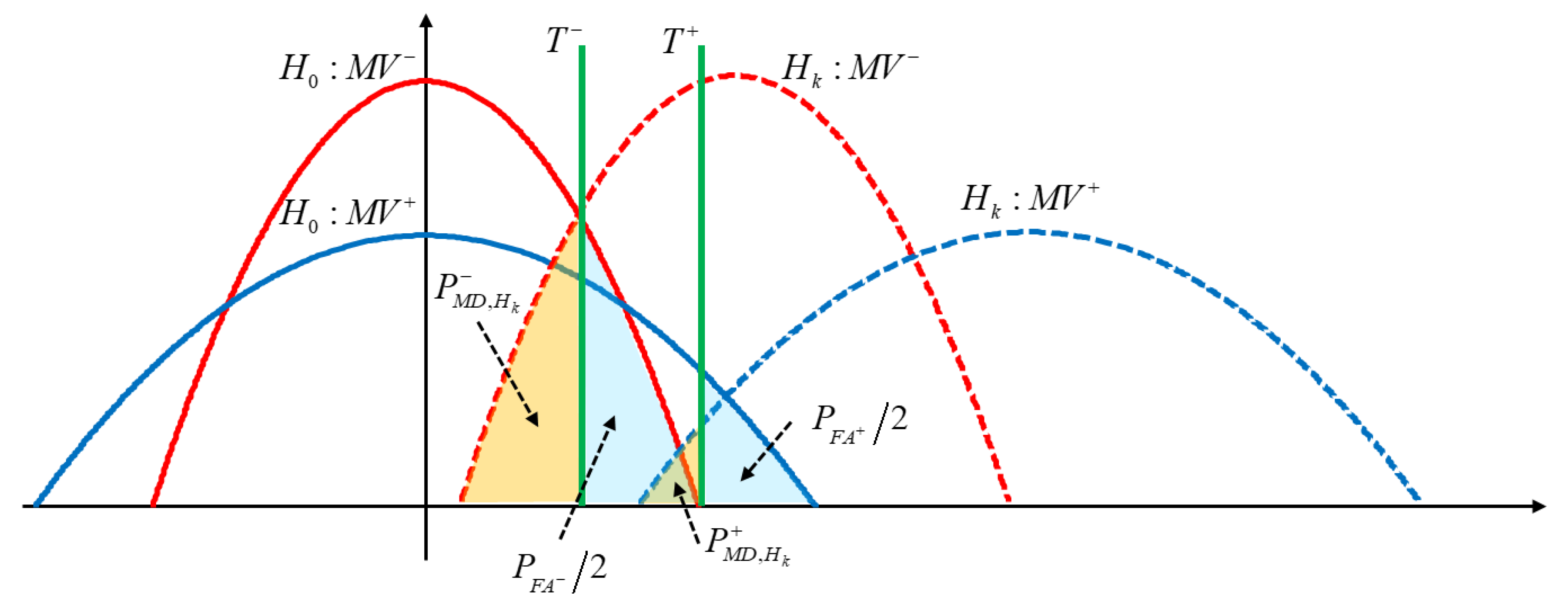
2.3.1. Probability of False Alarm and Probability of Missed Detection
2.3.2. Detection Threshold Determination
2.3.3. Probability of Missed Detection for Insensitive Cycle-Slip Pairs
2.4. Cycle-Slip Compensation Method
2.4.1. Cycle-Slip Identification Method
2.4.2. Cycle-Slip Validation Method
3. Algorithm Test Results
3.1. Algorithm Test Environment
3.2. Data Test Results
4. Conclusions
Author Contributions
Funding
Conflicts of Interest
References
- Song, J.; Park, B.; Kee, C. A Study on GPS/GLONASS Compact Network RTK and Analysis on Temporal Variations of Carrier Phase Corrections for Reducing Broadcast Bandwidth. In Proceedings of the ION 2017 Pacific PNT Meeting, Honolulu, HI, USA, 1–4 May 2017; pp. 659–669. [Google Scholar]
- Park, B. A Study on Reducing Temporal and Spatial Decorrelation Effect in GNSS Augmentation System: Consideration of the Correction Message Standardization. Ph.D. Thesis, Seoul National University, Seoul, Korea, 2008. [Google Scholar]
- Park, B.; Kee, C. The Compact Network RTK Method: An Effective Solution to Reduce GNSS Temporal and Spatial Decorrelation Error. J. Navig. 2010, 63, 343–362. [Google Scholar] [CrossRef]
- Song, J. A Study on Improving Performance of Network RTK through Tropospheric Modeling for Land Vehicle Applications. Ph.D. Thesis, Seoul National University, Seoul, Korea, 2016. [Google Scholar]
- Pullen, S. Augmented GNSS: Fundamentals and Keys to Integrity and Continuity. In Proceedings of the ION GNSS 2011 Tutorial, Portland, OR, USA, 19–23 September 2011. [Google Scholar]
- Teunissen, P.J.G. GNSS Integer Ambiguity Validation: Overview of Theory and Methods. In Proceedings of the ION 2013 Pacific PNT Meeting, Honolulu, HI, USA, 23–25 April 2013; pp. 673–684. [Google Scholar]
- Bisnath, S.B.; Kim, D.; Langley, R.B. A New Approach to an Old Problem: Carrier-Phase Cycle Slips. GPS World 2001, 13, 42–49. [Google Scholar]
- Seo, J.; Walter, T. Future Dual-Frequency GPS Navigation System for Intelligent Air Transportation under Strong Ionospheric Scintillation. IEEE Trans. Intell. Transp. Syst. 2014, 15, 2224–2236. [Google Scholar] [CrossRef]
- Luo, X.; Liu, Z.; Lou, Y.; Gu, S.; Chen, B. A Study of Multi-GNSS Ionospheric Scintillation and Cycle-Slip over Hong Kong Region for Moderate Solar Flux Conditions. Adv. Space Res. 2017, 60, 1039–1053. [Google Scholar] [CrossRef]
- Blewitt, G. An Automatic Editing Algorithm for GPS data. Geophys. Res. Lett. 1990, 17, 199–202. [Google Scholar] [CrossRef]
- Gao, Y.; Li, Z. Cycle Slip Detection and Ambiguity Resolution Algorithms for Dual-Frequency GPS Data Processing. Mar. Geodesy 1999, 22, 169–181. [Google Scholar]
- Liu, Z. A New Automated Cycle Slip Detection and Repair Method for a Single Dual-Frequency GPS Receiver. J. Geodesy 2011, 85, 171–183. [Google Scholar] [CrossRef]
- Cai, C.; Liu, Z.; Xia, P.; Dai, W. Cycle Slip Detection and Repair for Undifferenced GPS Observations under High Ionospheric Activity. GPS Solut. 2013, 17, 247–260. [Google Scholar] [CrossRef]
- Song, J.; Kee, C. A New Approach for GNSS Frequency Selection Considering Detection of Cycle Slip Insensitive Pairs of Ionospheric Combination for Dual- Frequency Receivers. In Proceedings of the 28th International Technical Meeting of The Satellite Division of the Institute of Navigation (ION GNSS+ 2015), Tampa, FL, USA, 14–18 September 2015; pp. 2681–2687. [Google Scholar]
- Liu, W.; Jin, X.; Wu, M.; Hu, J.; Wu, Y. A New Real-Time Cycle Slip Detection and Repair Method Under High Ionospheric Activity for a Triple-frequency GPS/BDS Receiver. Sensors 2018, 18, 427. [Google Scholar] [CrossRef] [PubMed]
- Zeng, T.; Sui, L.; Xu, Y.; Jia, X.; Xiao, G.; Tian, Y.; Zhang, Q. Real-Time Triple-Frequency Cycle Slip Detection and Repair Method Under Ionospheric Disturbance Validated with BDS Data. GPS Solut. 2018, 22, 1–13. [Google Scholar] [CrossRef]
- Zhang, X.; Li, P. Benefits of the Third Frequency Signal on Cycle Slip Correction. GPS Solut. 2016, 20, 451–460. [Google Scholar] [CrossRef]
- Dai, Z.; Knedlik, S.; Loffeld, O. Instantaneous Triple-Frequency GPS Cycle-Slip Detection and Repair. Int. J. Navig. Obs. 2009, 2009, 1–15. [Google Scholar] [CrossRef]
- Hu, C.; Wang, Q.; Wang, Z.; Moraleda, A.H. New-Generation BeiDou (BDS-3) Experimental Satellite Precise Orbit Determination with an Improved Cycle-Slip Detection and Repair Algorithm. Sensors 2018, 18, 1402. [Google Scholar] [CrossRef] [PubMed]
- Pu, R.; Xiong, Y. An Improved Algorithm Based on Combination Observations for Real Time Cycle Slip Processing in Triple Frequency BDS Measurements. Adv. Space Res. 2018. [Google Scholar] [CrossRef]
- Chang, G.; Xu, T.; Yao, Y.; Wang, Q. Adaptive Kalman Filter Based on Variance Component Estimation for the Prediction of Ionospheric Delay in Aiding the Cycle Slip Repair of GNSS Triple-Frequency Signals. J. Geodesy 2018, 92, 1–13. [Google Scholar] [CrossRef]
- Gu, X.; Zhu, B. Detection and Correction of Cycle Slip in Triple-Frequency GNSS Positioning. IEEE Access 2017, 5, 12584–12595. [Google Scholar] [CrossRef]
- Dach, R.; Lutz, S.; Walser, P.; Fridez, P. Bernese GNSS Software, version 5.2; Astronomical Institute, University of Bern: Bern, Switzerland, 2015; ISBN 978-3-906813-05-9. [Google Scholar]
- Chen, D.; Ye, S.; Zhou, W.; Liu, Y.; Jiang, P.; Tang, W.; Yuan, B.; Zhao, L. A Double-Differenced Cycle Slip Detection and Repair Method for GNSS CORS Network. GPS Solut. 2016, 20, 439–450. [Google Scholar] [CrossRef]
- Kee, C.; Walter, T.; Enge, P.; Parkinson, B. Quality Control Algorithms on WAAS Wide Area Reference Stations. Navig. J. Inst. Navig. 1997, 44, 53–62. [Google Scholar] [CrossRef]
- DeCleene, B. Defining Pseudorange Integrity—Overbounding. In Proceedings of the 13th International Technical Meeting of the Satellite Division of The Institute of Navigation (ION GPS 2000), Salt Lake City, UT, USA, 19–22 September 2000; pp. 1916–1924. [Google Scholar]
- Schempp, T.R.; Rubin, A.L. An Application of Gaussian Overbounding for the WAAS Fault Free Error Analysis. In Proceedings of the 15th International Technical Meeting of the Satellite Division of The Institute of Navigation (ION GPS 2002), Portland, OR, USA, 24–27 September 2002; pp. 766–772. [Google Scholar]
- Altmayer, C. Enhancing the integrity of integrated GPS/INS systems by cycle slip detection and correction. In Proceedings of the IEEE Intelligent Vehicles Symposium 2000, Dearborn, MI, USA, 3–5 October 2000; pp. 174–179. [Google Scholar]
- Song, J.; Kim, Y.; Yun, H.; Park, B.; Kee, C. Predictions of Allowable Sensor Error Limit for Cycle-Slip Detection. Trans. Jpn. Soc. Aeronaut. Space Sci. 2014, 57, 169–178. [Google Scholar] [CrossRef]
- Kim, Y.; Song, J.; Kee, C.; Park, B. GPS Cycle Slip Detection Considering Satellite Geometry based on TDCP/INS Integrated Navigation. Sensors 2015, 15, 25336–25365. [Google Scholar] [CrossRef] [PubMed]
- Teunissen, P.J.G.; De Jonge, P.J.; Tiberius, C.C.J.M. Performance of the LAMBDA Method for Fast GPS Ambiguity Resolution. Navig. J. Inst. Navig. 1997, 44, 373–383. [Google Scholar] [CrossRef]
- Hofmann-Wellenhof, B.; Lichtenegger, H.; Wasle, E. GNSS—Global Navigation Satellite Systems: GPS, GLONASS, Galileo, and More; Springer Science & Business Media: Berlin, Germany, 2008; ISBN 978-3-211-73012-6. [Google Scholar]
- Misra, P.; Enge, P. Global Positioning System: Signals, Measurements, and Performance, 2nd ed.; Ganga-Jamuna Press: Lincoln, MA, USA, 2006; ISBN 0-9709544-1-7. [Google Scholar]
- Li, B.; Lou, L.; Shen, Y. GNSS Elevation-Dependent Stochastic Modeling and Its Impacts on the Statistic Testing. J. Surv. Eng. 2015, 142, 04015012. [Google Scholar] [CrossRef]
- Olynik, M. Temporal Characteristics of GPS Error Sources and Their Impact on Relative Positioning. Master’s Thesis, The University of Calgary, Calgary, AB, Canada, 2002. [Google Scholar]
- Olynik, M.; Petovello, M.; Cannon, M.; Lachapelle, G. Temporal Impact of Selected GPS Errors on Point Positioning. GPS Solut. 2002, 6, 47–57. [Google Scholar]
- Park, B.; Kim, J.; Kee, C. RRC Unnecessary for DGPS Messages. IEEE Trans. Aerosp. Electron. Syst. 2006, 42, 1149–1160. [Google Scholar] [CrossRef]
- Tiwari, R.; Bhattacharya, S.; Purohitb, P.K.; Gwal, A.K. Effect of TEC Variation on GPS Precise Point at Low Latitude. Open Atmos. Sci. J. 2009, 3, 1–12. [Google Scholar] [CrossRef]
- Zhizhao, L.I.U.; Chen, W.U. Study of the Ionospheric TEC Rate in Hong Kong Region and its GPS/GNSS Application. In Global Navigation Satellite System: Technology Innovation and Application (CPGPS 2009); NAV Technology Co., Ltd.: Beijing, China, 2009; pp. 129–137. [Google Scholar]
- Kim, J.; Kee, C. RTK-GPS Correction Generation Technique for Low-Rate Data-Link. J. Navig. 2004, 57, 465–477. [Google Scholar] [CrossRef]
- Kim, D.; Langley, R.B. Instantaneous Real-Time Cycle-Slip Correction for Quality Control of GPS Carrier-Phase Measurements. Navig. J. Inst. Navig. 2002, 49, 205–222. [Google Scholar] [CrossRef]
- Kang, S.; Song, J.; Kim, O.; Kee, C. Analysis on Normal Ionospheric Trend and Detection of Ionospheric Disturbance by Earthquake. J. Adv. Navig. Technol. 2018, 22, 49–56. [Google Scholar]
- Zhang, W.; Zhao, X.; Jin, S.; Li, J. Ionospheric Disturbances Following the March 2015 Geomagnetic Storm from GPS Observations in China. Geodesy Geodyn. 2018, 9, 288–295. [Google Scholar] [CrossRef]
- Monti, K.L. Folded Empirical Distribution Function Curves-Mountain Plots. Am. Stat. 1995, 49, 342. [Google Scholar] [CrossRef]
- Joerger, M.; Pervan, B. Solution Separation and Chi-Squared ARAIM for Fault Detection and Exclusion. In Proceedings of the 2014 IEEE/ION Position, Location and Navigation Symposium, PLANS 2014, Monterey, CA, USA, 5–8 May 2014; pp. 294–307. [Google Scholar]
- Teunissen, P.J.G. Success Probability of Integer GPS Ambiguity Rounding and Bootstrapping. J. Geodesy 1998, 72, 606–612. [Google Scholar] [CrossRef]


| Combination | Number of Sample | Actual Sample Sigma | Theoretical Sigma | Bounding Scale Factor |
|---|---|---|---|---|
| Negative (IN) | 991,7379 | 4.6 mm/s2 | 15.1 mm/s2 | 3.3 |
| Positive (IP) | 991,7379 | 4.9 mm/s2 | 17.1 mm/s2 | 3.5 |
| Cycle Slip (Cycle) | Iono. Negative | Iono. Positive | Total | ||
|---|---|---|---|---|---|
| Bias (m) | PMD | Bias (m) | PMD | PMD | |
| (1, 0) | 0.294 | 3.1 × 10−50 | 0.095 | 0.156 | 4.9 × 10−51 |
| (0, 1) | 0.378 | 1.9 × 10−92 | 0.074 | 0.588 | 1.1 × 10−92 |
| (1, 1) | 0.083 | 0.174 | 0.169 | 4.3 × 10⁻⁸ | 7.5 × 10⁻⁹ |
| (−1, 1) | 0.672 | 0 | 0.021 | 1.000 | 0 |
| (−1, 2) | 1.049 | 0 | 0.053 | 0.928 | 0 |
| (−2, 2) | 1.343 | 0 | 0.042 | 0.982 | 0 |
| (−2, 3) | 1.721 | 0 | 0.032 | 0.996 | 0 |
| (−3, 3) | 2.015 | 0 | 0.063 | 0.809 | 0 |
| (−3, 4) | 2.392 | 0 | 0.011 | 1.000 | 0 |
| (−4, 5) | 3.064 | 0 | 0.001 | 1.000 | 0 |
| (4, 3) | 0.044 | 0.951 | 0.603 | 0 | 0 |
| (5, 4) | 0.039 | 0.976 | 0.772 | 0 | 0 |
| (8, 6) | 0.088 | 0.104 | 1.206 | 0 | 0 |
| (9, 7) | 0.005 | 1.000 | 1.375 | 0 | 0 |
| (10, 8) | 0.078 | 0.270 | 1.545 | 0 | 0 |
| Cycle Slip (Cycle) | General Method (IN + MW) | Proposed Method (IN + IP) |
|---|---|---|
| (1, 0) | 6.2 × 10−61 | 4.9 × 10−51 |
| (0, 1) | 0 | 1.1 × 10−92 |
| (1, 1) | 6.2 × 10⁻³ | 7.5 × 10⁻⁹ |
| (4, 3) | 0.497 | 0 |
| (5, 4) | 0.613 | 0 |
| (8, 6) | 9.5 × 10⁻⁴ | 0 |
| (9, 7) | 0.401 | 0 |
| (10, 8) | 5.9 × 10⁻³ | 0 |
| Date | 17 March 2015 |
|---|---|
| Time | UTC 06:00:00~11:59:59 (6 h) |
| Interval | 1 s |
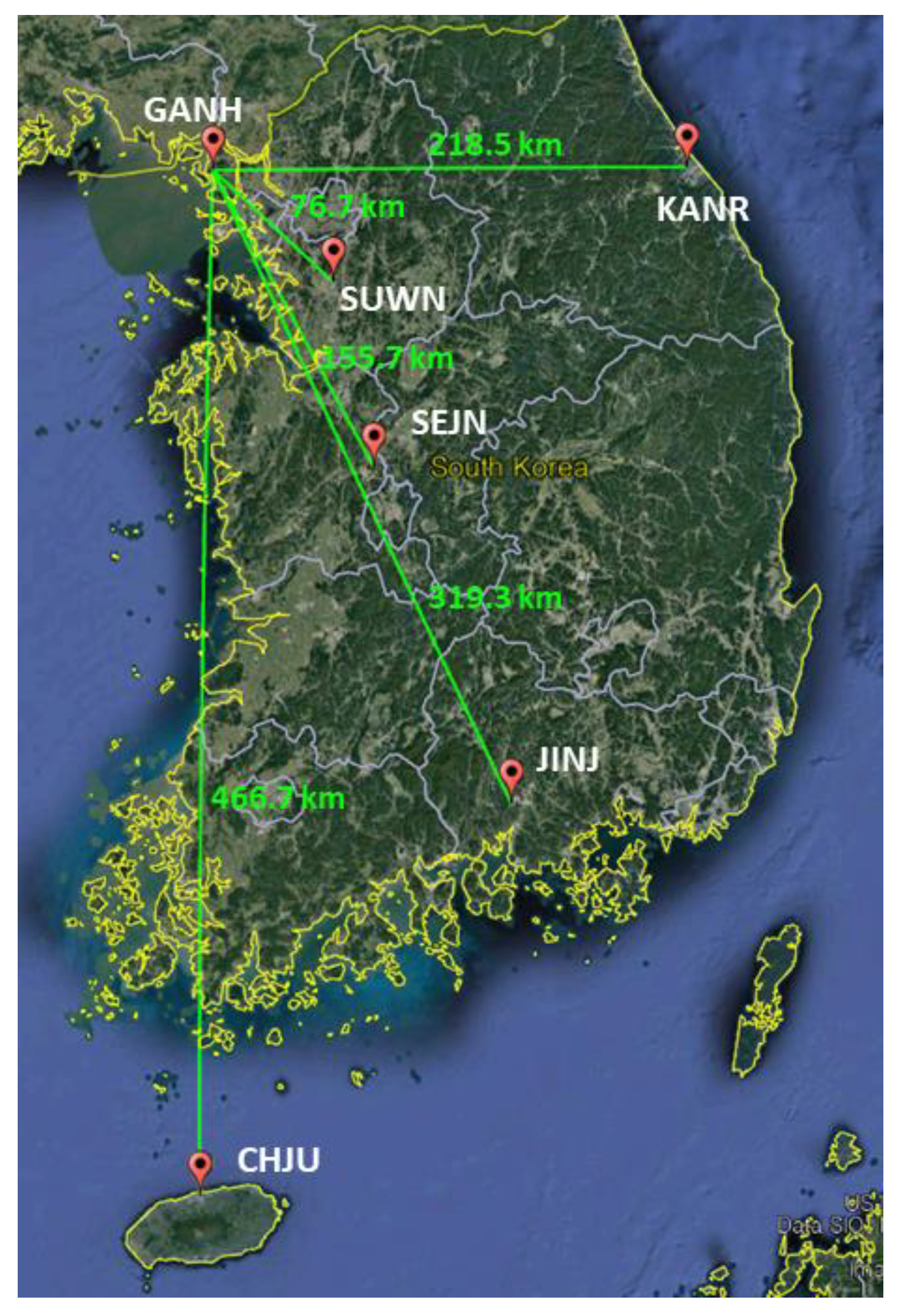
| Baseline | GANH–CHJU (467 km) |
| Receiver | Trimble NetR9 |
| Antenna | Trimble Zephyr (TRM59800) |
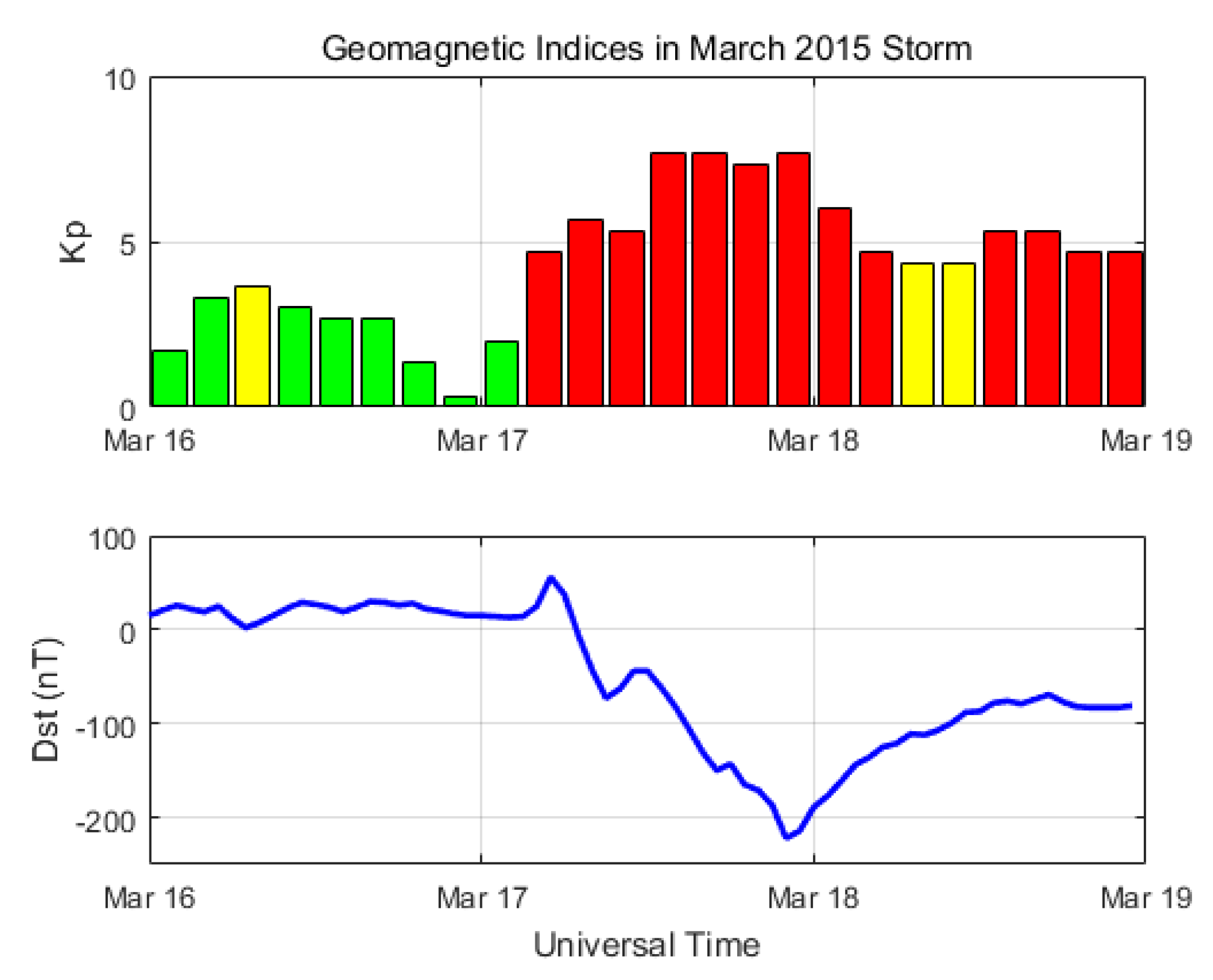
| Kp index | 8—(Daily maximum) |
| PRN | Epoch | El (°) | Inserted Cycle Slip (Cycle) | Monitoring Value (Meter) | Estimated CS (Cycle) | Validated Cycle Slip (cycle) | ||
|---|---|---|---|---|---|---|---|---|
| MV− | MV+ | L1 CS | L2 CS | |||||
| G14 | 10200 | 14.81 | (10, 8) | −0.083 | 1.553 | 10.029 | 8.029 | (10, 8) |
| 10300 | 14.09 | (5, 4) | −0.043 | 0.768 | 4.996 | 4.006 | (5, 4) | |
| 10400 | 13.37 | (−3, 4) | −2.403 | 0.024 | −2.943 | 4.062 | (−3, 4) | |
| 10500 | 12.65 | (−2, 2) | −1.341 | −0.039 | −1.998 | 2.011 | (−2, 2) | |
| 10600 | 11.94 | (0, 1) | −0.386 | 0.083 | 0.030 | 1.037 | (0, 1) | |
| 10700 | 11.22 | (1, 0) | 0.289 | 0.101 | 1.017 | 0.020 | (1, 0) | |
| 10800 | 10.52 | (1, 1) | −0.084 | 0.171 | 1.013 | 1.015 | (1, 1) | |
| G19 | 11600 | 5.99 | (1, 1) | −0.088 | 0.183 | 1.057 | 1.072 | (1, 1) |
| 11700 | 6.67 | (1, 0) | 0.291 | 0.103 | 1.017 | 0.012 | (1, 0) | |
| 11800 | 7.36 | (0, 1) | −0.385 | 0.070 | −0.051 | 0.979 | (0, 1) | |
| 11900 | 8.05 | (−1, 1) | −0.669 | −0.041 | −1.089 | 0.935 | (−1, 1) | |
| 12000 | 8.74 | (−2, 3) | −1.722 | 0.027 | −2.046 | 2.942 | (−2, 3) | |
| 12100 | 9.44 | (−4, 5) | −3.074 | −0.011 | −4.020 | 5.015 | (−4, 5) | |
| 12200 | 10.14 | (8, 6) | 0.091 | 1.193 | 7.956 | 5.952 | (8, 6) | |
| G27 | 7900 | 7.83 | (1, 1) | −0.090 | 0.166 | 0.941 | 0.948 | (1, 1) |
| 8000 | 8.52 | (1, 0) | 0.296 | 0.100 | 1.003 | −0.014 | (1, 0) | |
| 8100 | 9.20 | (0, 1) | −0.378 | 0.078 | 0.007 | 1.003 | (0, 1) | |
| 8200 | 9.90 | (−1, 2) | −1.047 | 0.059 | −0.980 | 2.010 | (−1, 2) | |
| 8300 | 10.59 | (−3, 3) | −2.020 | −0.063 | −3.011 | 2.981 | (−3, 3) | |
| 8400 | 11.29 | (4, 3) | 0.051 | 0.610 | 4.019 | 3.002 | (4, 3) | |
| 8500 | 11.99 | (9, 7) | 0.000 | 1.383 | 9.015 | 7.014 | (9, 7) | |
© 2018 by the authors. Licensee MDPI, Basel, Switzerland. This article is an open access article distributed under the terms and conditions of the Creative Commons Attribution (CC BY) license (http://creativecommons.org/licenses/by/4.0/).
Share and Cite
Kim, D.; Song, J.; Yu, S.; Kee, C.; Heo, M. A New Algorithm for High-Integrity Detection and Compensation of Dual-Frequency Cycle Slip under Severe Ionospheric Storm Conditions. Sensors 2018, 18, 3654. https://doi.org/10.3390/s18113654
Kim D, Song J, Yu S, Kee C, Heo M. A New Algorithm for High-Integrity Detection and Compensation of Dual-Frequency Cycle Slip under Severe Ionospheric Storm Conditions. Sensors. 2018; 18(11):3654. https://doi.org/10.3390/s18113654
Chicago/Turabian StyleKim, Donguk, Junesol Song, Sunkyoung Yu, Changdon Kee, and Moonbeom Heo. 2018. "A New Algorithm for High-Integrity Detection and Compensation of Dual-Frequency Cycle Slip under Severe Ionospheric Storm Conditions" Sensors 18, no. 11: 3654. https://doi.org/10.3390/s18113654
APA StyleKim, D., Song, J., Yu, S., Kee, C., & Heo, M. (2018). A New Algorithm for High-Integrity Detection and Compensation of Dual-Frequency Cycle Slip under Severe Ionospheric Storm Conditions. Sensors, 18(11), 3654. https://doi.org/10.3390/s18113654