Visual Object Tracking Using Structured Sparse PCA-Based Appearance Representation and Online Learning


Abstract
1. Introduction
- An appearance model that captures the visual characteristics of the target object and evaluates the similarity between observed samples and the model.
- A motion model that locates the target between successive frames utilizing certain motion hypotheses.
- An optimization strategy that associates the appearance model with the motion model and finds the most likely location in the current frame.
- Structured sparse PCA-based appearance representation and learning for efficient description of the target object with few dictionary entries, to reduce the high-dimensional descriptor and to retain the structure.
- Local structure enforced similarity measures to avoid problems from partial occlusion, illumination and background clutter.
- Training image selection for robust online dictionary learning and updating by considering the probability that the training image contains the target, as opposed to the existing methods that choose the most recent training images.
2. Review of Previous Related Work
2.1. Visual Object Tracking System
2.2. Sparse Representation-Based Learning
3. Structured Sparse PCA-Based Tracking and Online Dictionary Learning
3.1. Notations and Symbols
3.2. Bayesian Framework-Based Visual Object Tracking
- (i)
- State is independent of the past given the present ,
- (ii)
- Observations are conditionally independent given ,
- structured sparse PCA-based observation and appearance representation using deterministic target object separation from background patch images,
- motion tracking and
- online update.
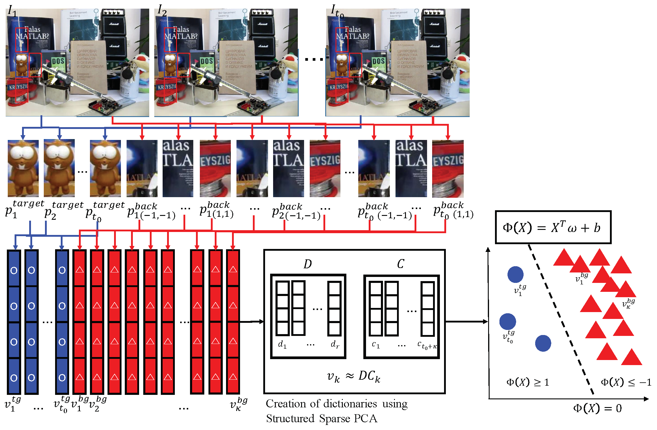
3.3. Deterministic Modeling Using Structured Sparse PCA-Based Appearance Representation
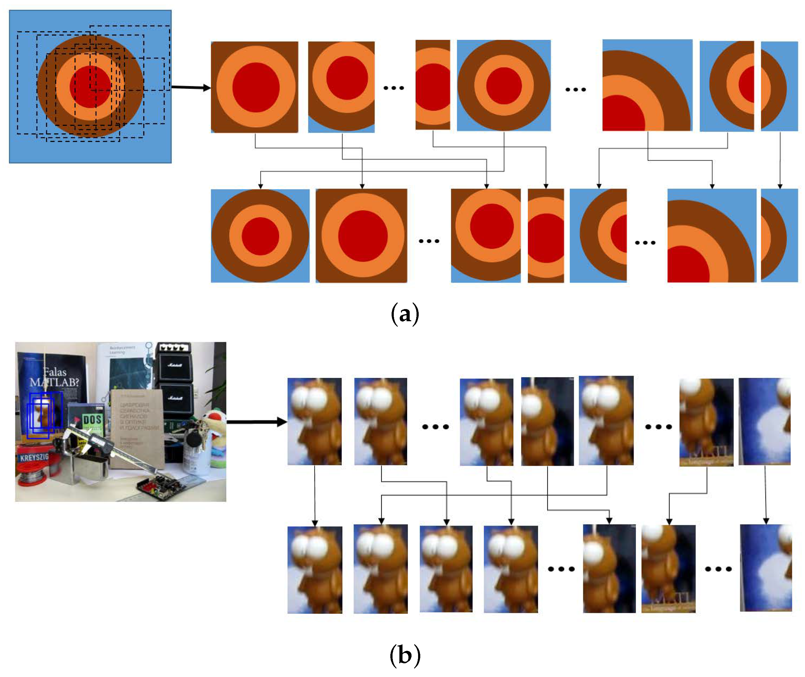
- We take the same sized image patches centered at from frames respectively.Recall that states consist of the center location of the target and its window size in the x and y directions, respectively. From each patch we construct the descriptor of the target object by sequentially accumulating gradient histograms from equally-divided subregions of .To enhance tracking performance, we also create background feature descriptors from the four background patch images around the target patch as follows.
- For each , patches are subimages of centered at with the same size as .
- When the domain of does not entirely belong to that of , we regard it as an empty set.
- Let with be background appearance descriptors obtained from background patches in the same manner used to create the target descriptors.
- After creating the appearance feature descriptors and , we apply the constrained structured sparse PCA dictionary learning algorithm to the target and background descriptors to find dictionaries ,where the objective function is given by:and is the matrix with and column vectors; is the dictionary matrix; and is the coefficient matrix, such that for , is (approximately or exactly) expressed by a linear combination of with coefficients ,for
- Let be the Frobenius matrix norm, , for ; the Euclidean norm; and a quasi-norm that controls the sparsity and structure of the support of In this work, the quasi-norm is defined as follows. Let be four mutually disjoint subsets of Then, every vector is decomposed into four subvectors such that for andThen, is defined as:We refer to [49] and the references therein for details on the quasi-norm. The decomposition of V into enables us to reduce the dimensionality of the descriptors using Equation (6).Although there is clearly a limitation in representing high dimensional descriptors using a smaller number of vectors than the dimension, the proposed structured sparse PCA is more effective to represent nonlinear and high dimensional descriptors by reducing the dimension while retaining the target object structure. For more details of structured sparse PCA algorithms, refer to the original paper [49].
- Finally, we find a linear support vector machine (SVM) , such that for the target feature-related column vectors of and for the background appearance feature related column vectors of , where denotes the i-th column vector of , i.e., Using the classifier , we estimate observation as:where we recall that is the target feature descriptor obtained from state . Note that when the target object is occluded or not observed, the value of the observation becomes negative.
| Algorithm 1: Discriminative classification of target objects. |
Input: frame images , states , integers
|
| Output: target appearance descriptors and classifier |
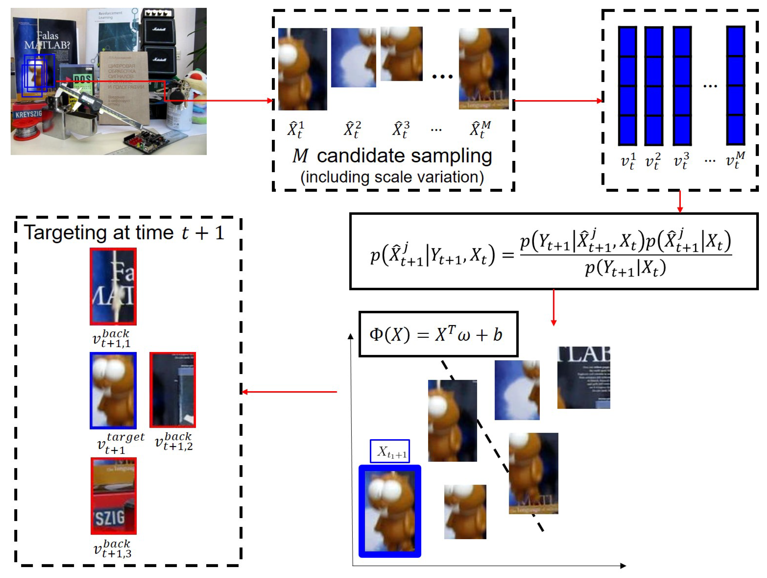
3.4. Motion Tracking Model and Online Update
| Algorithm 2: Motion tracking model. |
for to the end of the frame sequence
|
| end |
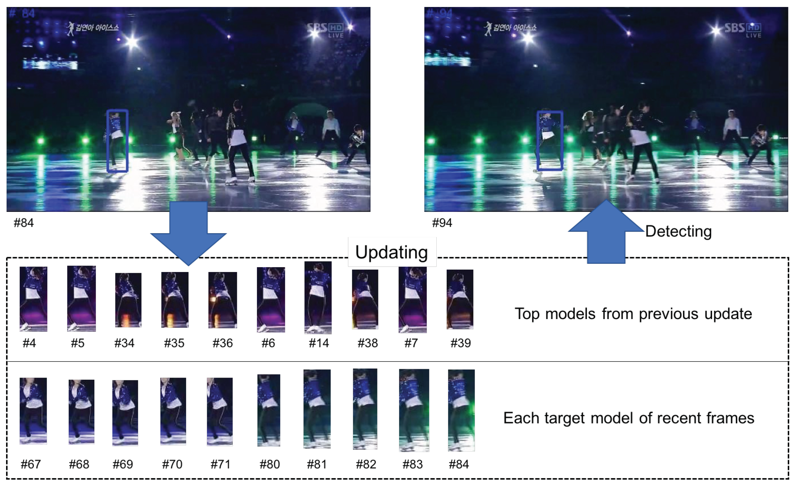
- We save the target descriptors into a set at time .
- At every , if , we add the target descriptor and background descriptors to F. Otherwise, .
- After every k frames, we create the dictionary matrix and coefficient matrix using the vectors in F by applying the structured sparse PCA.
- Similar to the initiation algorithm, we update using the new and .
- We check for all target descriptors and sort the descriptors according to their values, while keeping the largest target descriptors in F and deleting the remaining target descriptors and all the background descriptors from F.
| Algorithm 3: Dictionary update. |
| for to the end of the frame sequence |
| 1. if |
| 1-1. add the target descriptor |
| and background descriptors to F |
| 1. else |
| 1-2. |
| for every k frames |
| 2. build the new metrics and using the vectors in F |
| by structured sparse PCA |
| 3. update classifier using and |
| 4. compute for |
| 5. keep the largest target descriptors in F, |
| and delete the rest descriptor from F |
| 6. |
| end |
4. Experimental Validation
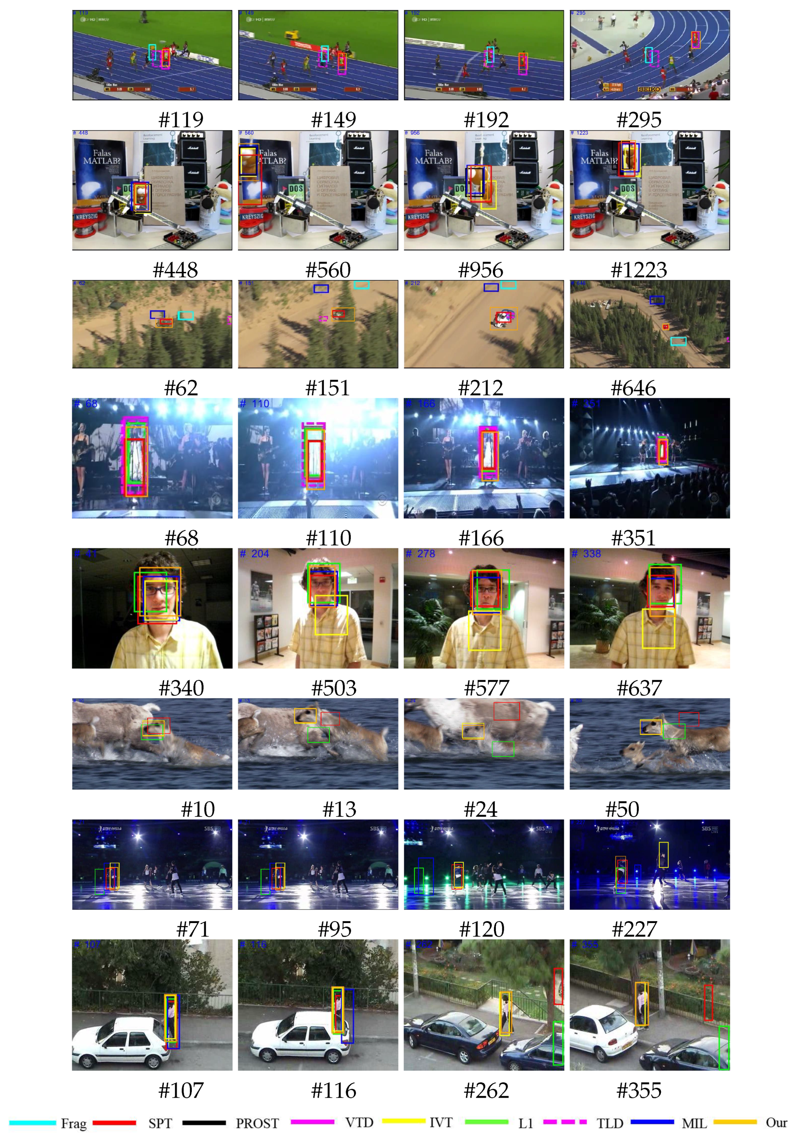
4.1. Qualitative Analysis
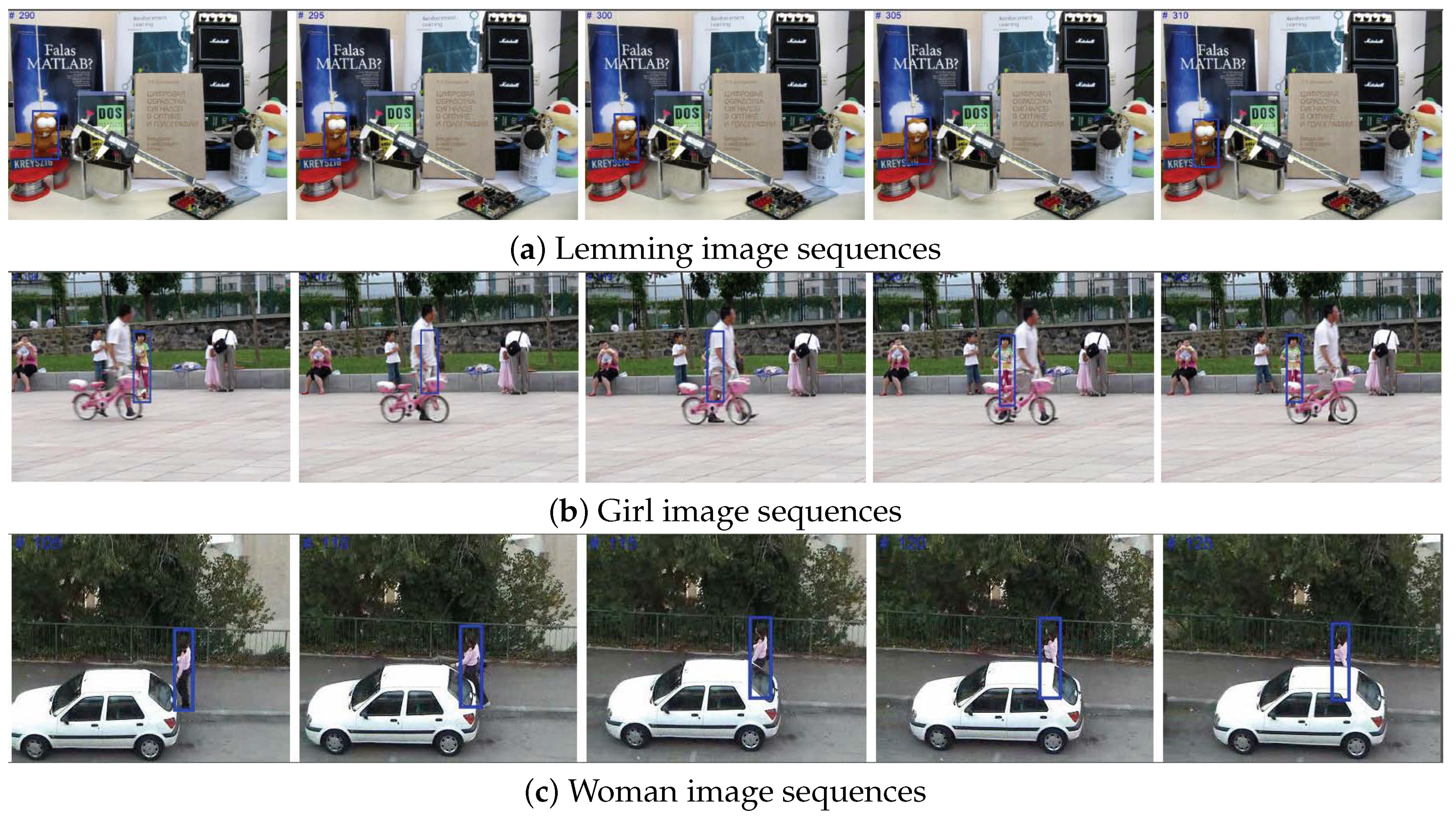
4.1.1. Significant Occlusion
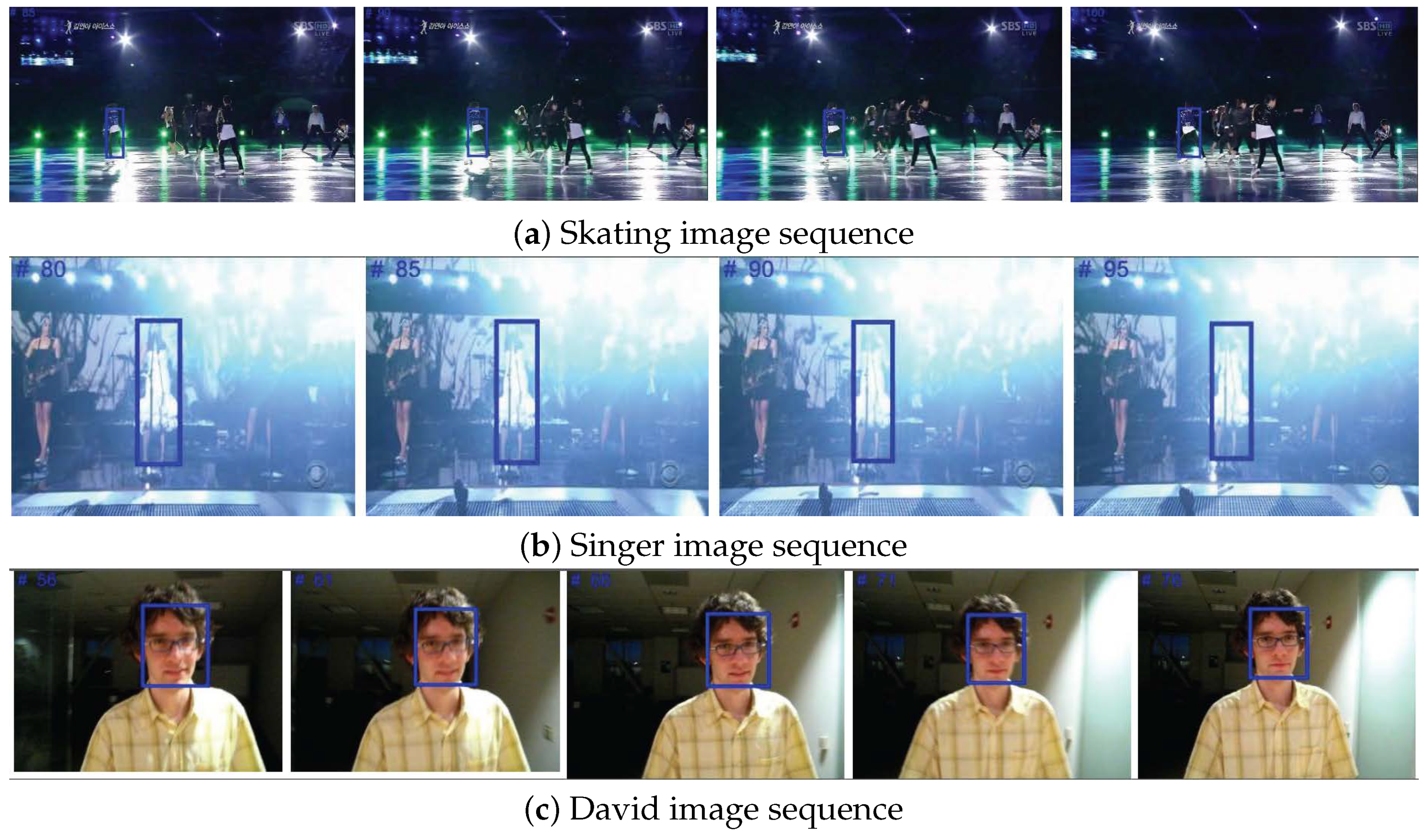
4.1.2. Illumination Change
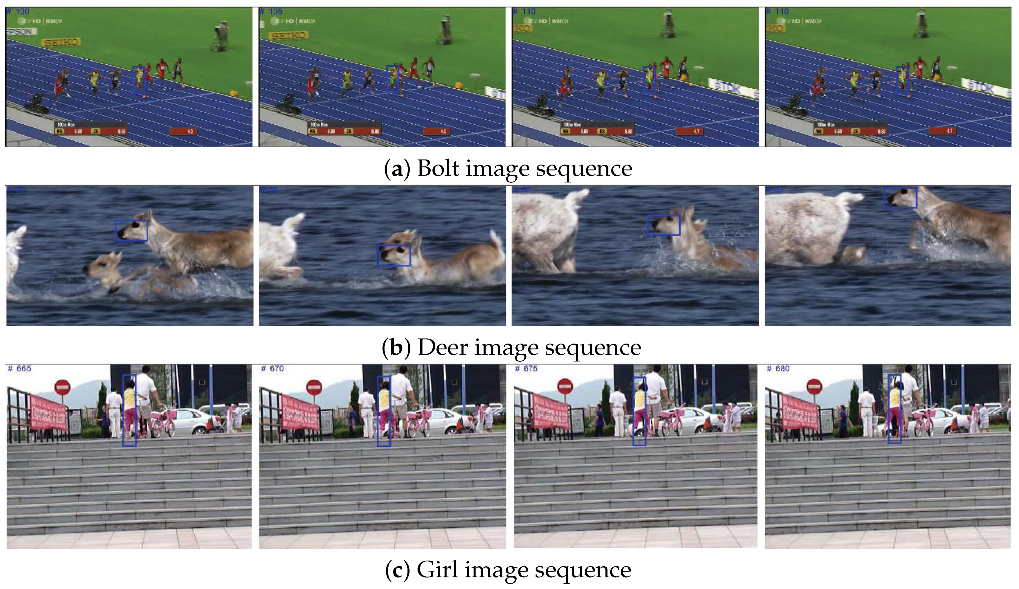
4.1.3. Background Clutter
4.2. Quantitative Analysis
5. Conclusions
Author Contributions
Funding
Conflicts of Interest
References
- Trucco, E.; Plakas, K. Video tracking: A concise survey. IEEE J. Ocean. Eng. 2006, 31, 520–529. [Google Scholar] [CrossRef]
- Yilmaz, A.; Javed, O.; Shah, M. Object tracking. ACM Comput. Surv. 2006, 38, 1–45. [Google Scholar] [CrossRef]
- Jalal, A.S.; Singh, V. The State-of-the-Art in Visual Object Tracking. Informatica 2012, 36, 227–248. [Google Scholar]
- Smeulders, A.W.M.; Chu, D.M.; Cucchiara, R.; Calderara, S.; Dehghan, A.; Shah, M. Visual tracking: An experimental survey. IEEE Trans. Pattern Anal. Mach. Intell. 2014, 36, 1442–1468. [Google Scholar] [PubMed]
- Wu, Y.; Lim, J.; Yang, M.H. Online object tracking: A benchmark. In Proceedings of the IEEE Computer Society Conference on Computer Vision and Pattern Recognition, Portland, OR, USA, 23–28 June 2013; pp. 2411–2418. [Google Scholar]
- Wu, Y.; Lim, J.; Yang, M.H. Object tracking benchmark. IEEE Trans. Pattern Anal. Mach. Intell. 2015, 37, 1834–1848. [Google Scholar] [CrossRef] [PubMed]
- Beymer, D.; McLauchlan, P.; Coifman, B.; Malik, J. A real-time computer vision system for measuring traffic parameters. In Proceedings of the IEEE Computer Society Conference on Computer Vision and Pattern Recognition, San Juan, Puerto Rico, 17–19 June 1997; pp. 495–501. [Google Scholar]
- Li, X.; Hu, W.; Shen, C.; Zhang, Z.; Dick, A.; van den Hengel, A. A Survey of Appearance Models in Visual Object Tracking. ACM Trans. Intell. Syst. Technol. 2013, 4, 1–42. [Google Scholar] [CrossRef]
- Chen, F.; Wang, Q.; Wang, S.; Zhang, W.; Xu, W. Object tracking via appearance modeling and sparse representation. Image Vis. Comput. 2011, 29, 787–796. [Google Scholar] [CrossRef]
- Bai, T.; Li, Y.F. Robust visual tracking with structured sparse representation appearance model. Pattern Recognit. 2012, 45, 2390–2404. [Google Scholar] [CrossRef]
- Jia, X.; Lu, H.; Yang, M.H. Visual tracking via adaptive structural local sparse appearance model. In Proceedings of the IEEE Computer Society Conference on Computer Vision and Pattern Recognition, Providence, RI, USA, 16–21 June 2012; pp. 1822–1829. [Google Scholar]
- Rubinstein, R.; Bruckstein, A.M.; Elad, M. Dictionaries for sparse representation modeling. Proc. IEEE 2010, 98, 1045–1057. [Google Scholar] [CrossRef]
- Sadeghi, M.; Babaie-Zadeh, M.; Jutten, C. Dictionary learning for sparse decomposition: A novel approach. IEEE Signal Process. Lett. 2013, 20, 1195–1198. [Google Scholar] [CrossRef]
- Huang, T. Linear spatial pyramid matching using sparse coding for image classification. In Proceedings of the 2009 IEEE Conference on Computer Vision and Pattern Recognition, Miami, FL, USA, 20–25 June 2009; pp. 1794–1801. [Google Scholar]
- Henrigues, J.F.; Caseiro, R.; Martins, P.; Batista, J. High-Speed Tracking with Kernelized Correlation Filters. IEEE Trans. Pattern Anal. Mach. Intell. 2015, 37, 583–596. [Google Scholar] [CrossRef] [PubMed]
- Birchfield, S.T. KLT: An Implementation of the Kanade-Lucas-Tomasi Feature Tracker. Available online: https://cecas.clemson.edu/~stb/klt/ (accessed on 17 October 2018).
- Kalman, R.E. A new approach to linear filtering and prediction problems. J. Basic Eng. 1960, 82, 35–45. [Google Scholar] [CrossRef]
- Ramos, J.A. A kalman-tracking filter approach to nonlinear programming. Comput. Math. Appl. 1990, 19, 63–74. [Google Scholar] [CrossRef]
- Comaniciu, D.; Ramesh, V.; Meer, P. Real-time tracking of non-rigid objects using mean shift. In Proceedings of the IEEE Conference on Computer Vision and Pattern Recognition, Hilton Head, SC, USA, 13–15 June 2000; Volume 2, pp. 142–149. [Google Scholar]
- Allen, J.G.; Xu, R.Y.D.; Jin, J.S. Object Tracking Using CamShift Algorithm and Multiple Quantized Feature Spaces. Reproduction 2006, 36, 3–7. [Google Scholar]
- Khan, Z.; Balch, T.; Dellaert, F. An MCMC-Based Particle Filter for Tracking Multiple Interacting Targets. In European Conference on Computer Vision; Springer: Berlin/Heidelberg, Germany, 2004; pp. 279–290. [Google Scholar]
- Babenko, B.; Yang, M.H.; Belongie, S.J. Visual tracking with online multiple instance learning. In Proceedings of the IEEE Conference on Computer Vision and Pattern Recognition, Miami, FL, USA, 20–25 June 2009; pp. 983–990. [Google Scholar]
- Maraghi, T.F.E.; Fleet, D.J.; Jepson, A.D. Robust online appearance models for visual tracking. In Proceedings of the the IEEE Conference on Computer Vision and Pattern Recognition, Kauai, HI, USA, 8–14 December 2001; pp. 415–422. [Google Scholar]
- Ross, D.A.; Lim, J.W.; Lin, R.S.; Yang, M.H. Incremental learning for robust visual tracking. Int. J. Comput. Vis. 2008, 77, 125–141. [Google Scholar] [CrossRef]
- Srikrishnan, V.; Nagaraj, T.; Chaudhuri, S. Fragment based tracking for scale and orientation adaptation. In Proceedings of the Indian Conference on Computer Vision, Graphics and Image Processing, Bhubaneswar, India, 16–19 December 2008; pp. 328–335. [Google Scholar]
- Kalal, Z.; Matas, J.; Mikolajczyk, K. P-N learning: Bootstrapping. In Proceedings of the IEEE Computer Society Conference on Computer Vision and Pattern Recognition, San Francisco, CA, USA, 13–18 June 2010; pp. 49–56. [Google Scholar]
- Kalal, Z.; Mikolajczyk, K.; Matas, J. Tracking-learning-detection. IEEE Trans. Pattern Anal. Mach. Intell. 2012, 34, 1409–1422. [Google Scholar] [CrossRef] [PubMed]
- Hare, S.; Saffari, A.; Torr, P.H.S. Struck: Structured output tracking with kernels. In Proceedings of the International Conference on Computer Vision, Barcelona, Spain, 6–13 November 2011; pp. 263–270. [Google Scholar]
- Zhong, W.; Lu, H.; Yang, M.H. Robust object tracking via sparse collaborative appearance model. IEEE Trans. Image Process. 2014, 23, 2356–2368. [Google Scholar] [CrossRef] [PubMed]
- Kwon, J.; Lee, K.M. Visual tracking decomposition. In Proceedings of the IEEE Computer Society Conference on Computer Vision and Pattern Recognition, San Francisco, CA, USA, 13–18 June 2010; pp. 1269–1276. [Google Scholar]
- Bao, C.; Wu, Y.; Ling, H.; Ji, H. Real time robust L1 tracker using accelerated proximal gradient approach. In Proceedings of the IEEE Computer Society Conference on Computer Vision and Pattern Recognition, Providence, RI, USA, 16–21 June 2012; pp. 1830–1837. [Google Scholar]
- Zhang, T.; Liu, S.; Xu, C.; Yan, S.; Ghanem, B.; Ahuja, N.; Yang, M.-H. Structural Sparse Tracking. In Proceedings of the 2015 IEEE Conference on Computer Vision and Pattern Recognition (CVPR), Boston, MA, USA, 7–12 June 2015; pp. 150–158. [Google Scholar]
- Zhang, T.; Ghanem, B.; Liu, S.; Ahuja, N. Robust Visual Tracking via Structured Multi-Task Sparse Learning. Int. J. Comput. Vis. 2017, 101, 367–383. [Google Scholar] [CrossRef]
- Chen, Z.; You, X.; Zhong, B.; Li, J. Dynamically Modulated Mask Sparse Tracking. IEEE Trans. Cybern. 2017, 47, 3706–3718. [Google Scholar] [CrossRef] [PubMed]
- Wang, N.; Yeung, D.-Y. Learning a deep compact image representation for visual tracking. In Proceedings of the Neural Information Processing Systems, Lake Tahoe, NV, USA, 5–10 December 2013; pp. 809–817. [Google Scholar]
- Hong, S.; You, T.; Kwak, S.; Han, B. Online tracking by learning discriminative saliency map with convolutional neural network. In Proceedings of the International Conference on Machine Learning, Lille, France, 6–11 July 2015. [Google Scholar]
- Zhang, D.; Maei, H.; Wang, X.; Fang, Y. Deep Reinforcement Learning for Visual Object Tracking. arXiv, 2017; arXiv:1701.08936. [Google Scholar]
- Nam, H.; Han, B. Learning Multi-Domain Convolutional Neural Networks for Visual Tracking. In Proceedings of the IEEE Conference on Computer Vision and Pattern Recognition (CVPR), Honolulu, HI, USA, 21–26 July 2017. [Google Scholar]
- Wang, L.; Ouyang, W.; Wang, X.; Lu, H. STCT: Sequentially Training Convolutional Networks for Visual Tracking. In Proceedings of the 2016 IEEE Conference on Computer Vision and Pattern Recognition (CVPR), Las Vegas, NV, USA, 27–30 June 2016. [Google Scholar]
- Yang, F.; Lu, H.; Yang, M.-H. Robust superpixel tracking. IEEE Trans. Image Process. 2014, 23, 1639–1651. [Google Scholar] [CrossRef] [PubMed]
- Donoho, D.L. Compressed sensing. IEEE Trans. Inf. Theory 2006, 52, 1289–1306. [Google Scholar] [CrossRef]
- Candes, E.; Wakin, M. An introduction to compressive sensing. IEEE Signal Process. Mag. 2008, 25, 21–30. [Google Scholar] [CrossRef]
- Cheng, H. Sparse Representation, Modeling and Learning in Visual Recognition—Theory, Algorithms and Applications; Series Advances in Computer Vision and Pattern Recognition; Springer: New York, NY, USA, 2015. [Google Scholar]
- Kreutz-Delgado, K.; Murray, J.F.; Rao, B.D.; Engan, K.; Lee, T.-W.; Sejnowski, T.J. Dictionary learning algorithms for sparse representation. Neural Comput. 2003, 15, 349–396. [Google Scholar] [CrossRef] [PubMed]
- Wright, J.; Ma, Y.; Mairal, J.; Sapiro, G.; Huang, T.S.; Yan, S. Sparse representation for computer vision and pattern recognition. Proc. IEEE 2010, 98, 1031–1044. [Google Scholar] [CrossRef]
- Elhamifar, E.; Vidal, R. Robust classification using structured sparse representation. In Proceedings of the IEEE Conference on Computer Vision and Pattern Recognition (CVPR), Colorado Springs, CO, USA, 20–25 June 2011; pp. 1873–1879. [Google Scholar]
- Bronstein, A.M.; Sprechmann, P.; Sapiro, G. Learning efficient structured sparse models. arXiv, 2012; arXiv:1206.4649. [Google Scholar]
- Varshney, K.R.; Çetin, M.J.W.; Fisher, J.W., III; Willsky, A.S. Sparse representation in structured dictionaries with application to synthetic aperture radar. IEEE Trans. Signal Process. 2008, 56, 3548–3561. [Google Scholar] [CrossRef]
- Jenatton, R.; Obozinski, G.; Bach, F.R. Structured sparse principal component analysis. In Proceedings of the Thirteenth International Conference on Artificial Intelligence and Statistics (AISTATS), Sardinia, Italy, 13–15 May 2010; pp. 66–373. [Google Scholar]
- Lowe, D.G. Distinctive Image Features from Scale-Invariant Keypoints. Int. J. Comput. Vis. 2004, 60, 91–110. [Google Scholar] [CrossRef]


| Symbol | Description |
|---|---|
| Frame at time t | |
| State variable | |
| Observation variable | |
| Location vector in the state variable | |
| Target descriptor vector | |
| Background descriptor vector | |
| Patch image | |
| Column vectors of D | |
| Column vectors of C | |
| V | Feature descriptor |
| D | Feature dictionary |
| C | Feature coefficient matrices |
| Support vector machine classifier | |
| Diagonal covariance matrix | |
| Multivariate normal distribution | |
| F | Set of target descriptors |
| p | Probability function |
| s | Dimension of descriptors |
| r | Number of dictionary vectors |
| Number of background descriptors | |
| k | Number of vectors after updating |
| t | Time variable |
| Real number or 1 related to width size | |
| Real number or 1 related to height size | |
| Width (x-axis) size of patch | |
| Height (y-axis) size of patch | |
| ≈ | Approximately equal |
| ∝ | Proportional to |
| Transpose operator |
| All | BC | DEF | FM | IPR | IV | LR | MB | OCC | OPR | OV | SV | |
|---|---|---|---|---|---|---|---|---|---|---|---|---|
| Proposed | 58.50 | 60.19 | 58.78 | 56.74 | 56.22 | 52.03 | 60.86 | 58.96 | 55.00 | 57.13 | 56.51 | 52.33 |
| VTD [30] | 49.3 | 55.1 | 46.2 | 41.7 | 50.2 | 53.7 | 47.1 | 43.5 | 52.3 | 53.7 | 51.5 | 48.9 |
| MS [19] | 35.6 | 36.7 | 32.8 | 40.5 | 36.8 | 34.6 | 28.4 | 41.2 | 37.4 | 37.3 | 41.0 | 36.0 |
| MIL [22] | 45.9 | 48.6 | 45.7 | 44.1 | 45.7 | 47.1 | 43.5 | 43.7 | 47.6 | 48.9 | 52.7 | 44.5 |
| SCM [29] | 54.4 | 61.3 | 51.5 | 42.8 | 51.8 | 61.1 | 61.7 | 45.2 | 56.8 | 57.0 | 56.4 | 55.8 |
| Frag [25] | 44.2 | 46.1 | 41.8 | 44.8 | 43.3 | 42.6 | 42.6 | 46.1 | 46.6 | 46.1 | 50.1 | 44.2 |
| IVT [24] | 46.4 | 51.6 | 40.5 | 37.3 | 46.4 | 51.2 | 55.8 | 41.3 | 49.3 | 49.0 | 52.3 | 47.1 |
| TLD [27] | 46.8 | 48.3 | 37.4 | 44.6 | 48.9 | 46.7 | 53.3 | 51.0 | 45.2 | 46.0 | 50.2 | 47.1 |
| Struct [28] | 57.5 | 59.3 | 52.4 | 55.6 | 57.0 | 59.0 | 59.1 | 59.9 | 55.9 | 57.3 | 58.9 | 57.8 |
| ASLA [11] | 53.2 | 59.2 | 50.5 | 42.0 | 52.1 | 59.6 | 59.3 | 44.6 | 56.0 | 56.3 | 55.3 | 54.0 |
© 2018 by the authors. Licensee MDPI, Basel, Switzerland. This article is an open access article distributed under the terms and conditions of the Creative Commons Attribution (CC BY) license (http://creativecommons.org/licenses/by/4.0/).
Share and Cite
Yoon, G.-J.; Hwang, H.J.; Yoon, S.M. Visual Object Tracking Using Structured Sparse PCA-Based Appearance Representation and Online Learning. Sensors 2018, 18, 3513. https://doi.org/10.3390/s18103513
Yoon G-J, Hwang HJ, Yoon SM. Visual Object Tracking Using Structured Sparse PCA-Based Appearance Representation and Online Learning. Sensors. 2018; 18(10):3513. https://doi.org/10.3390/s18103513
Chicago/Turabian StyleYoon, Gang-Joon, Hyeong Jae Hwang, and Sang Min Yoon. 2018. "Visual Object Tracking Using Structured Sparse PCA-Based Appearance Representation and Online Learning" Sensors 18, no. 10: 3513. https://doi.org/10.3390/s18103513
APA StyleYoon, G.-J., Hwang, H. J., & Yoon, S. M. (2018). Visual Object Tracking Using Structured Sparse PCA-Based Appearance Representation and Online Learning. Sensors, 18(10), 3513. https://doi.org/10.3390/s18103513