Value of Information Based Data Retrieval in UWSNs

 , and
, and 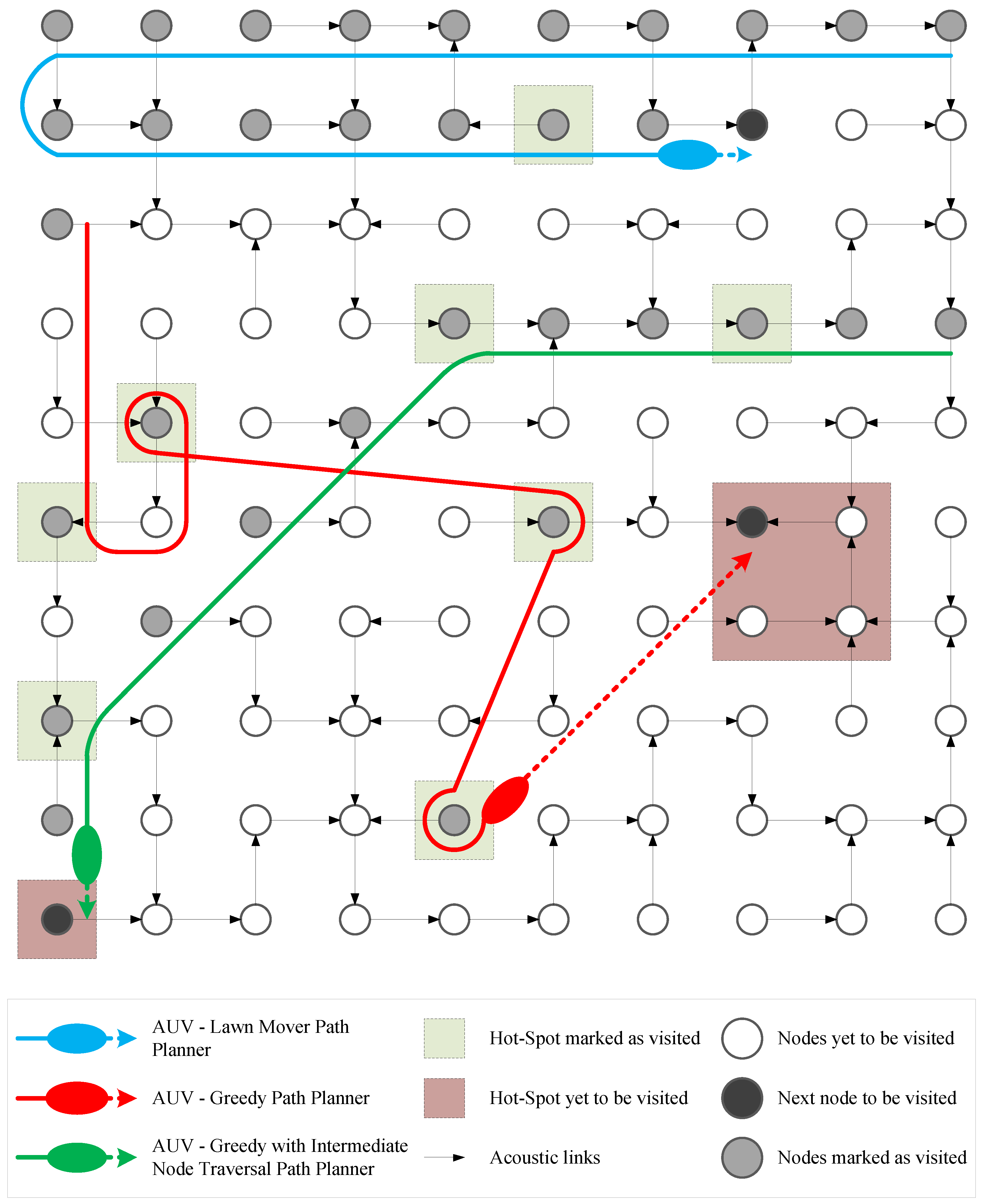
Abstract
1. Introduction
2. Related Work
2.1. Relationship between QoS, QoI, VoI and Routing
2.2. Some Applications of IQ and VoI in Sensor Networks
2.3. Using Mobile Sinks in Underwater Sensor Networks
2.4. AUV Path Planning
3. Value of Information in Underwater Sensor Networks
3.1. Value of Information
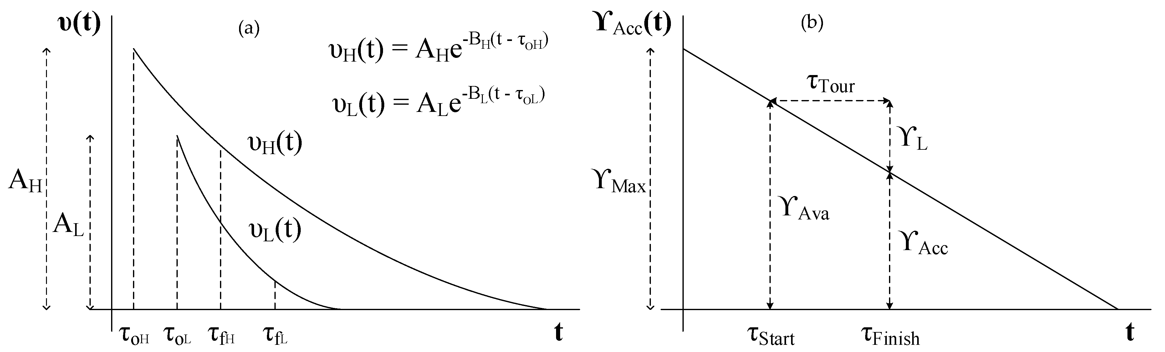
3.2. Temporality of VoI; Infotentials
3.3. UWSN Deployment Scenario
3.4. Problem Definition
3.4.1. VoI Maximization
3.4.2. Role of in Infotentials
3.4.3. The Path Planning Problem
- is the node visitation sequence determined by ,
- is a path planning algorithm that generates path such that is accumulated,
- S is the set of all sensor nodes,
- D is the set of all data reports,
- is the cumulative VoI function.
4. Path Planning Algorithms
4.1. Lawn-Mower Path Planner–LPP
| Algorithm 1 Shortest Path Lawn-Mower Path Planner–LPP. | |
| 1: procedure LPP(S) | |
| 2: | ▹ Set of sensor nodes |
| 3: | ▹ Visitation sequence |
| 4: | ▹ Direction priority list |
| 5: | ▹ Tour starting node |
| 6: while do | |
| 7: neighborhood() | |
| 8: from N in the direction given by | |
| 9: tourEculidean() | |
| 10: | |
| 11: | |
| 12: | |
| 13: end while | |
| 14: return V | |
| 15: end procedure | |
4.2. Greedy Path Planner–GPP
| Algorithm 2 Greedy Path Planner–GPP. | |
| 1: procedure GPP(S, ) | |
| 2: | ▹ Set of sensor nodes |
| 3: | ▹ Visitation sequence |
| 4: | ▹ Tour starting node |
| 5: while do | |
| 6: getNodeThatHasMaxVoI(S) | |
| 7: tourEculidean() | |
| 8: | |
| 9: | |
| 10: end while | |
| 11: return V | |
| 12: end procedure | |
| 13: procedure getNodeThatHasMaxVoI() | |
| 14: determine using DetermineNodeVoI(, t) | |
| 15: such that is | |
| 16: return k | |
| 17: end procedure | |
| 18: procedure DetermineNodeVoI() | |
| 19: | ▹ Data reports at node |
| 20: | |
| 21: | ▹ AUV arrival time at node |
| 22: while do | |
| 23: GetNextDataReport(D) | |
| 24: Get(j) | |
| 25: Get(j) | |
| 26: Get(j) | |
| 27: | |
| 28: | |
| 29: end while | |
| 30: end procedure | |
4.3. Greedy Path Planner with Intermediate-Node-Visitation–GIPP
| Algorithm 3 Greedy Path Planner with Intermediate-Node-Visitation–GIPP. | |
| 1: procedure GIPP(S, ) | |
| 2: | ▹ Set of sensor nodes |
| 3: | ▹ Visitation sequence |
| 4: | ▹ Tour starting node |
| 5: while do | |
| 6: getNodeThatHasMaxVoI(S) | |
| 7: | |
| 8: tourIntermediate() | |
| 9: | |
| 10: | |
| 11: | |
| 12: end while | |
| 13: return V | |
| 14: end procedure | |
| 15: procedure tourIntermediate() | |
| 16: | |
| 17: | |
| 18: | ▹ Intermediate Visitation Sequence |
| 19: while do | |
| 20: getNeighborhood() | |
| 21: such that eculideanDistance() is minimized | |
| 22: tourEculidean() | |
| 23: | |
| 24: | |
| 25: end while | |
| 26: return | |
| 27: end procedure | |
4.4. Hybrid Path Planner–HPP
| Algorithm 4 Hybrid Path planner–HPP. | |
| 1: procedure HPP(S, ) | |
| 2: | ▹ Set of sensor nodes |
| 3: | ▹ Visitation sequence |
| 4: is high-priority} | ▹ Set of high-priority sensor nodes |
| 5: | ▹ Set of low-priority sensor nodes |
| 6: GPP(, ) | |
| 7: LPP() | |
| 8: return V | |
| 9: end procedure | |
4.5. Hybrid Path Planner with Intermediate-Node-Visitation–HIPP
| Algorithm 5 Hybrid Path Planner with Intermediate-Node-Visitation–HIPP. | |
| 1: procedure HIPP(S, ) | |
| 2: | ▹ Set of sensor nodes |
| 3: | ▹ Visitation sequence |
| 4: is high-priority } | ▹ Set of high-priority sensor nodes |
| 5: | ▹ Sensor node to start tour from |
| 6: while do | |
| 7: getNodeMaxVoI() | |
| 8: | |
| 9: tourIntermediate() | |
| 10: | |
| 11: | |
| 12: | |
| 13: end while | |
| 14: | ▹ Set low-priority sensor nodes |
| 15: V + LPP() | |
| 16: return V | |
| 17: end procedure | |
4.6. Random Path Planner–RPP
5. Performance Measures, Simulation Setup and Results
5.1. Performance Measures and Experiments
5.2. Simulation Setup
5.3. Results
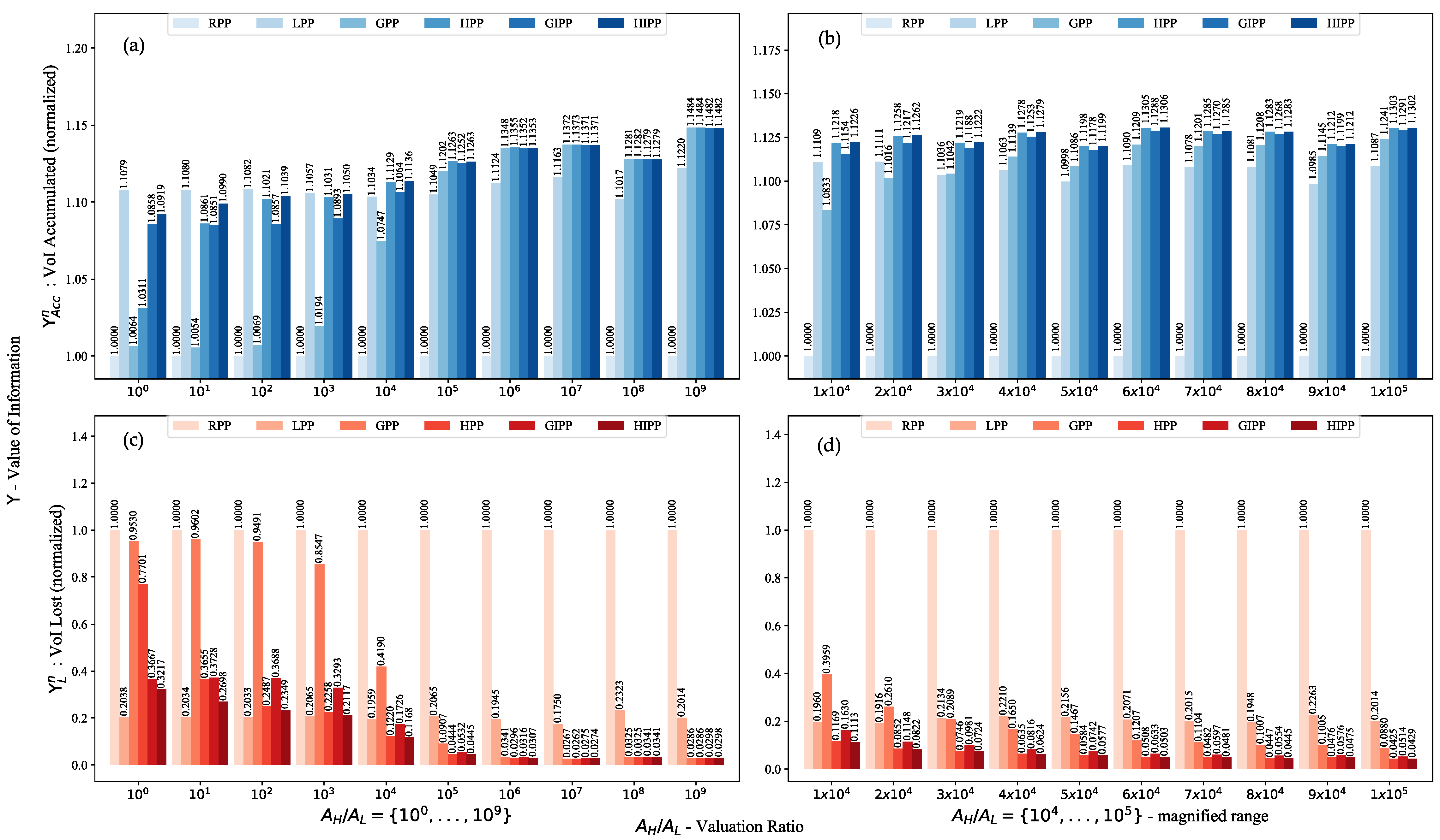
5.3.1. Valuation Ratio
5.3.2. Justification of Heuristics
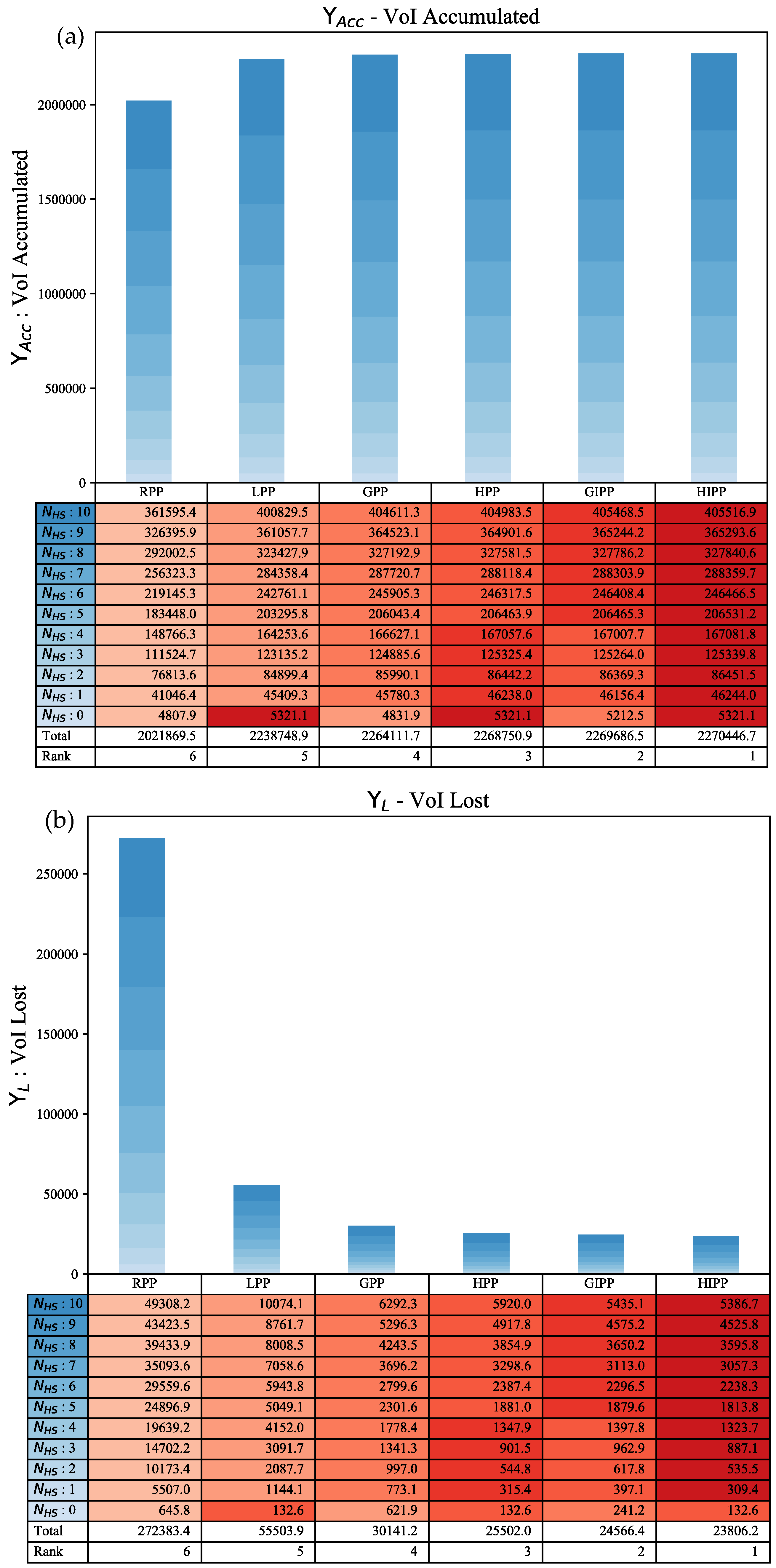
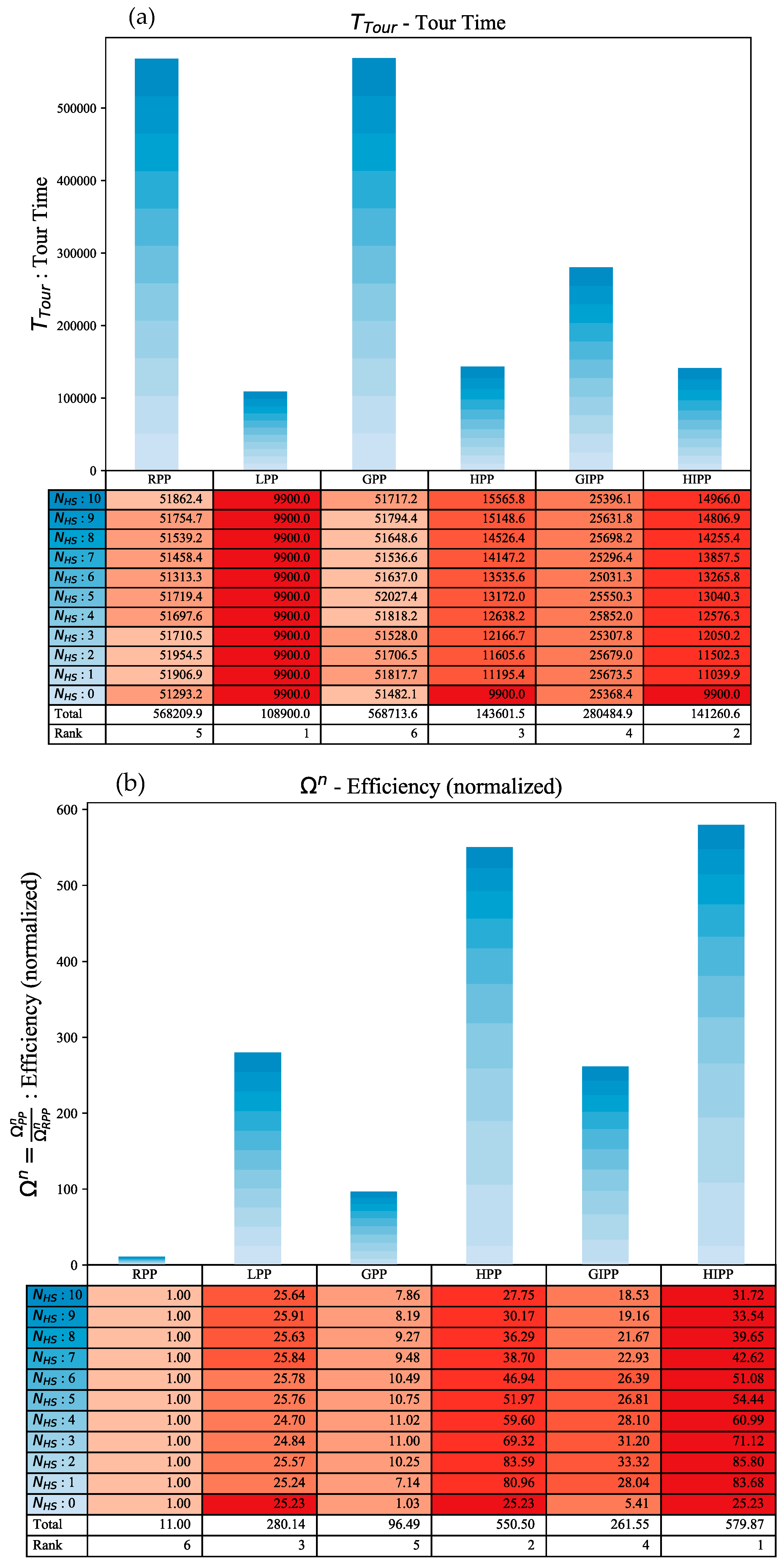
5.3.3. Comparative Analysis
VoI Accumulated and VoI Lost
Tour Time
Efficiency
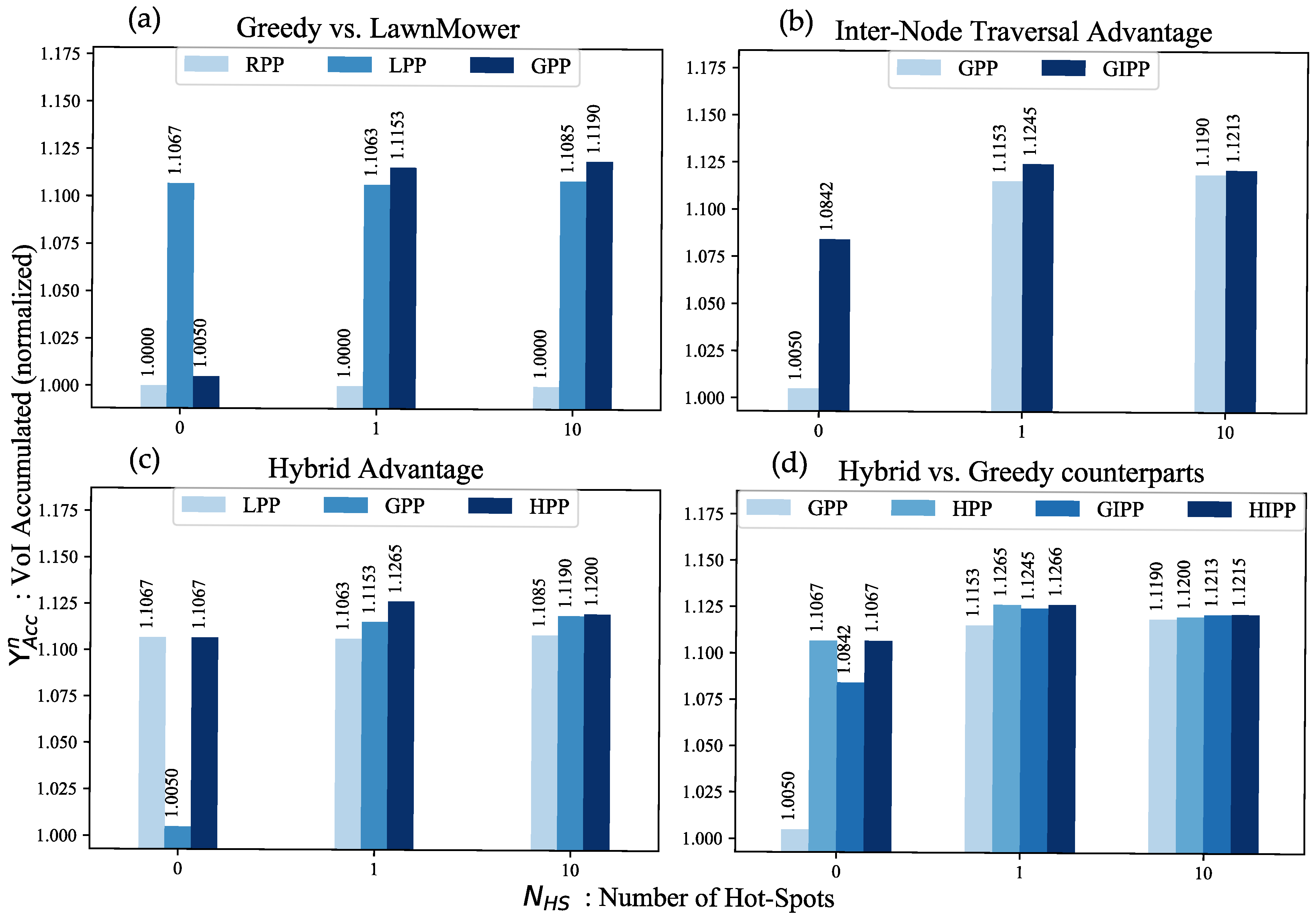
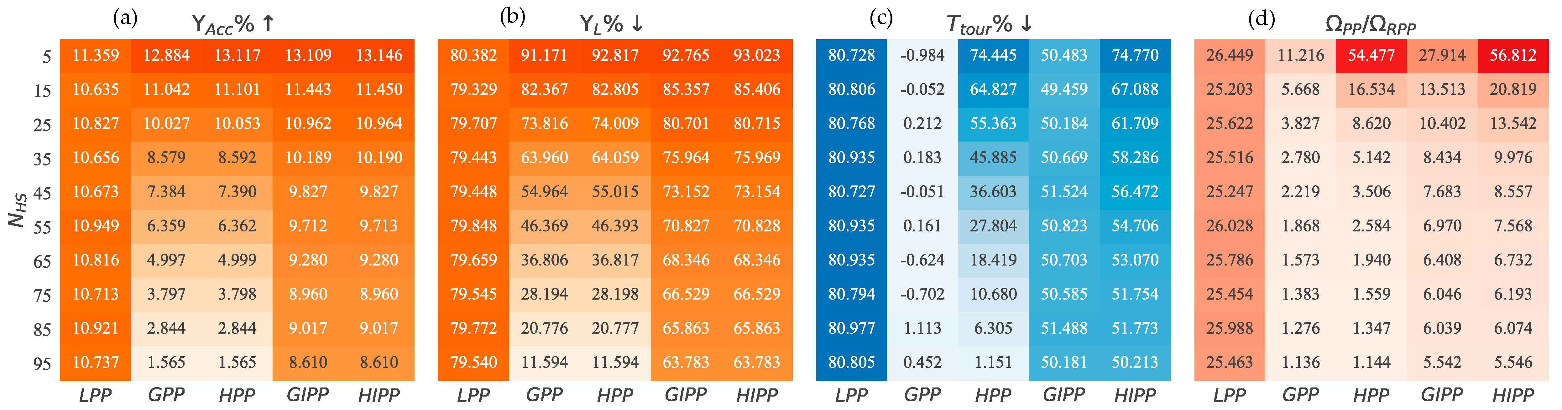
5.3.4. Scalability with an Increase in Hot-Spots
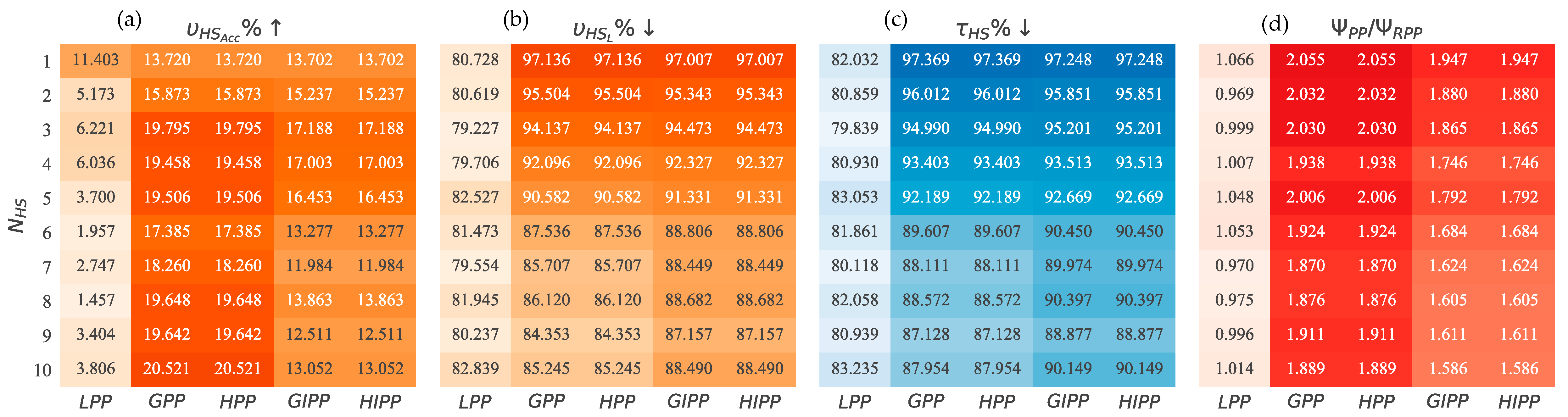
5.3.5. Response to Emergency
6. Conclusions
Author Contributions
Funding
Conflicts of Interest
References
- Akyildiz, I.F.; Pompili, D.; Melodia, T. Underwater acoustic sensor networks: Research challenges. Ad Hoc Netw. 2005, 3, 257–279. [Google Scholar] [CrossRef]
- Heidemann, J.; Stojanovic, M.; Zorzi, M. Underwater sensor networks: Applications, advances and challenges. Philos. Trans. R. Soc. A 2012, 370, 158–175. [Google Scholar] [CrossRef] [PubMed]
- Lv, C.; Wang, Q.; Yan, W.; Shen, Y. Energy-balanced compressive data gathering in Wireless Sensor Networks. J. Netw. Comput. Appl. 2016, 61, 102–114. [Google Scholar] [CrossRef]
- Ayaz, M.; Baig, I.; Abdullah, A.; Faye, I. A survey on routing techniques in underwater wireless sensor networks. J. Netw. Comput. Appl. 2011, 34, 1908–1927. [Google Scholar] [CrossRef]
- Esch, R.R.; Protti, F.; Barbosa, V.C. Adaptive event sensing in networks of autonomous mobile agents. J. Netw. Comput. Appl. 2016, 71, 118–129. [Google Scholar] [CrossRef]
- Vasilescu, I.; Kotay, K.; Rus, D.; Dunbabin, M.; Corke, P. Data collection, storage, and retrieval with an underwater sensor network. In Proceedings of the 3rd International Conference on Embedded Networked Sensor Systems, San Diego, CA, USA, 2–4 November 2005; pp. 154–165. [Google Scholar]
- Forero, P.A.; Lapic, S.K.; Wakayama, C.; Zorzi, M. Rollout algorithms for data storage-and energy-aware data retrieval using autonomous underwater vehicles. In Proceedings of the International Conference on Underwater Networks & Systems, Rome, Italy, 12–14 November 2014; p. 22. [Google Scholar]
- Khan, J.U.; Cho, H.S. A distributed data-gathering protocol using AUV in underwater sensor networks. Sensors 2015, 15, 19331–19350. [Google Scholar] [CrossRef] [PubMed]
- Akbar, M.; Javaid, N.; Khan, A.H.; Imran, M.; Shoaib, M.; Vasilakos, A. Efficient data gathering in 3D linear underwater wireless sensor networks using sink mobility. Sensors 2016, 16, 404. [Google Scholar] [CrossRef] [PubMed]
- Hollinger, G.A.; Choudhary, S.; Qarabaqi, P.; Murphy, C.; Mitra, U.; Sukhatme, G.S.; Stojanovic, M.; Singh, H.; Hover, F. Underwater Data Collection Using Robotic Sensor Networks. IEEE J. Sel. Areas Commun. 2012, 30, 899–911. [Google Scholar] [CrossRef]
- Farr, N.; Bowen, A.; Ware, J.; Pontbriand, C.; Tivey, M. An integrated, underwater optical/acoustic communications system. In Proceedings of the OCEANS 2010 IEEE-Sydney, Sydney, Australia, 24–27 May 2010; pp. 1–6. [Google Scholar]
- Khan, F.A.; Khan, S.A.; Turgut, D.; Bölöni, L. Greedy path planning for maximizing value of information in underwater sensor networks. In Proceedings of the IEEE 39th Conference on Local Computer Networks Workshops (LCN Workshops), Edmonton, AB, Canada, 8–11 September 2014; pp. 610–615. [Google Scholar]
- Bisdikian, C.; Kaplan, L.M.; Srivastava, M.B.; Thornley, D.J.; Verma, D.; Young, R.I. Building principles for a quality of information specification for sensor information. In Proceedings of the 12th International Conference on Information Fusion, Seattle, WA, USA, 6–9 July 2009; pp. 1370–1377. [Google Scholar]
- Bisdikian, C.; Branch, J.; Leung, K.K.; Young, R.I. A letter soup for the quality of information in sensor networks. In Proceedings of the 2009 IEEE International Conference on Pervasive Computing and Communications, Galveston, TX, USA, 9–13 March 2009; pp. 1–6. [Google Scholar]
- Bisdikian, C.; Kaplan, L.M.; Srivastava, M.B. On the quality and value of information in sensor networks. ACM Trans. Sens. Netw. 2013, 9, 48. [Google Scholar] [CrossRef]
- Chen, D.; Varshney, P.K. QoS Support in Wireless Sensor Networks: A Survey. In Proceedings of the International Conference on Wireless Networks, Las Vegas, NV, USA, 21–24 June 2004; Volume 233, pp. 1–7. [Google Scholar]
- Singh, G.T.; Al-Turjman, F.M. A data delivery framework for cognitive information-centric sensor networks in smart outdoor monitoring. Comput. Commun. 2016, 74, 38–51. [Google Scholar] [CrossRef]
- Aurrecoechea, C.; Campbell, A.T.; Hauw, L. A survey of QoS architectures. Multimed. Syst. 1998, 6, 138–151. [Google Scholar] [CrossRef]
- Al-Karaki, J.N.; Kamal, A.E. Routing techniques in wireless sensor networks: A survey. IEEE Wirel. Commun. 2004, 11, 6–28. [Google Scholar] [CrossRef]
- Akkaya, K.; Younis, M. A survey on routing protocols for wireless sensor networks. Ad Hoc Netw. 2005, 3, 325–349. [Google Scholar] [CrossRef]
- Ehsan, S.; Hamdaoui, B. A survey on energy-efficient routing techniques with QoS assurances for wireless multimedia sensor networks. IEEE Commun. Surv. Tutor. 2012, 14, 265–278. [Google Scholar] [CrossRef]
- Hasan, M.Z.; Al-Rizzo, H.; Al-Turjman, F. A survey on multipath routing protocols for QoS assurances in real-time wireless multimedia sensor networks. IEEE Commun. Surv. Tutor. 2017, 19, 1424–1456. [Google Scholar] [CrossRef]
- Hanzo, L.; Tafazolli, R. A survey of QoS routing solutions for mobile ad hoc networks. IEEE Commun. Surv. Tutor. 2007, 9, 50–70. [Google Scholar] [CrossRef]
- Chen, L.; Heinzelman, W.B. A survey of routing protocols that support QoS in mobile ad hoc networks. IEEE Netw. 2007, 21. [Google Scholar] [CrossRef]
- Gubbi, J.; Buyya, R.; Marusic, S.; Palaniswami, M. Internet of Things (IoT): A vision, architectural elements, and future directions. Future Gener. Comput. Syst. 2013, 29, 1645–1660. [Google Scholar] [CrossRef]
- Bonomi, F.; Milito, R.; Zhu, J.; Addepalli, S. Fog computing and its role in the internet of things. In Proceedings of the First Edition of the MCC workshop on Mobile cloud computing, Helsinki, Finland, 17 August 2012; pp. 13–16. [Google Scholar]
- Rosário, D.; Zhao, Z.; Santos, A.; Braun, T.; Cerqueira, E. A beaconless opportunistic routing based on a cross-layer approach for efficient video dissemination in mobile multimedia IoT applications. Comput. Commun. 2014, 45, 21–31. [Google Scholar] [CrossRef]
- Airehrour, D.; Gutierrez, J.; Ray, S.K. Secure routing for internet of things: A survey. J. Netw. Comput. Appl. 2016, 66, 198–213. [Google Scholar] [CrossRef]
- Chu, M.; Haussecker, H.; Zhao, F. Scalable information-driven sensor querying and routing for ad hoc heterogeneous sensor networks. Int. J. High Perform. Comput. Appl. 2002, 16, 293–313. [Google Scholar] [CrossRef]
- Zhao, F.; Shin, J.; Reich, J. Information-driven dynamic sensor collaboration. IEEE Signal Process. Mag. 2002, 19, 61–72. [Google Scholar] [CrossRef]
- Shen, H.; Bai, G. Routing in wireless multimedia sensor networks: A survey and challenges ahead. J. Netw. Comput. Appl. 2016, 71, 30–49. [Google Scholar] [CrossRef]
- Tan, H.X.; Chan, M.C.; Xiao, W.; Kong, P.Y.; Tham, C.K. Information quality aware routing in event-driven sensor networks. In Proceedings of the 2010 Proceedings IEEE INFOCOM, San Diego, CA, USA, 14–19 March 2010; pp. 1–9. [Google Scholar]
- Turgut, D.; Bölöni, L. A pragmatic value-of-information approach for intruder tracking sensor networks. In Proceedings of the 2012 IEEE International Conference on Communications (ICC), Ottawa, ON, Canada, 10–15 June 2012; pp. 4931–4936. [Google Scholar]
- Turgut, D.; Bölöni, L. IVE: Improving the value of information in energy-constrained intruder tracking sensor networks. In Proceedings of the 2013 IEEE International Conference on Communications (ICC), Budapest, Hungary, 9–13 June 2013; pp. 6360–6364. [Google Scholar]
- Pryyma, V.; Turgut, D.; Bölöni, L. Active time scheduling for rechargeable sensor networks. Comput. Netw. 2010, 54, 631–640. [Google Scholar] [CrossRef]
- Nasser, N.; Karim, L.; Taleb, T. Dynamic multilevel priority packet scheduling scheme for wireless sensor network. IEEE Trans. Wirel. Commun. 2013, 12, 1448–1459. [Google Scholar] [CrossRef]
- Huang, L.; Neely, M.J. Utility optimal scheduling in energy-harvesting networks. IEEE/ACM Trans. Netw. 2013, 21, 1117–1130. [Google Scholar] [CrossRef]
- Yu, X.; Xiaosong, X.; Wenyong, W. Priority-based low-power task scheduling for wireless sensor network. In Proceedings of the 2009 International Symposium on Autonomous Decentralized Systems, Athens, Greece, 23–25 March 2009; pp. 1–5. [Google Scholar]
- Hao, H.; Wang, K.; Ji, H.; Li, X.; Zhang, H. Utility-based scheduling algorithm for wireless multi-media sensor networks. In Proceedings of the 2015 IEEE 26th Annual International Symposium on Personal, Indoor, and Mobile Radio Communications (PIMRC), Hong Kong, China, 30 August–2 September 2015; pp. 1052–1056. [Google Scholar]
- Yigitel, M.A.; Incel, O.D.; Ersoy, C. QoS-aware MAC protocols for wireless sensor networks: A survey. Comput. Netw. 2011, 55, 1982–2004. [Google Scholar] [CrossRef]
- Kim, H.; Min, S.G. Priority-based QoS MAC protocol for wireless sensor networks. In Proceedings of the 2009 IEEE International Symposium on Parallel & Distributed Processing, Rome, Italy, 23–29 May 2009; pp. 1–8. [Google Scholar]
- He, L.; Pan, J.; Xu, J. A progressive approach to reducing data collection latency in wireless sensor networks with mobile elements. IEEE Trans. Mob. Comput. 2013, 12, 1308–1320. [Google Scholar] [CrossRef]
- Gu, Y.; Ren, F.; Ji, Y.; Li, J. The evolution of sink mobility management in wireless sensor networks: A survey. IEEE Commun. Surv. Tutor. 2016, 18, 507–524. [Google Scholar] [CrossRef]
- Sugihara, R.; Gupta, R.K. Speed control and scheduling of data mules in sensor networks. ACM Trans. Sens. Netw. 2010, 7, 4. [Google Scholar] [CrossRef]
- Sugihara, R.; Gupta, R.K. Path planning of data mules in sensor networks. ACM Trans. Sens. Netw. 2011, 8, 1. [Google Scholar] [CrossRef]
- Magistretti, E.; Kong, J.; Lee, U.; Gerla, M.; Bellavista, P.; Corradi, A. A mobile delay-tolerant approach to long-term energy-efficient underwater sensor networking. In Proceedings of the 2007 IEEE Wireless Communications and Networking Conference, Kowloon, China, 11–15 March 2007; pp. 2866–2871. [Google Scholar]
- Bölöni, L.; Turgut, D.; Basagni, S.; Petrioli, C. Scheduling data transmissions of underwater sensor nodes for maximizing value of information. In Proceedings of the 2013 IEEE Global Communications Conference (GLOBECOM), Atlanta, GA, USA, 9–13 December 2013; pp. 438–443. [Google Scholar]
- Gjanci, P.; Petrioli, C.; Basagni, S.; Phillips, C.A.; Bölöni, L.; Turgut, D. Path finding for maximum value of information in multi-modal underwater wireless sensor networks. IEEE Trans. Mob. Comput. 2018, 17, 404–418. [Google Scholar] [CrossRef]
- Khan, F.A.; Khan, S.A.; Turgut, D.; Bölöni, L. Scheduling multiple mobile sinks in Underwater Sensor Networks. In Proceedings of the IEEE 40th Conference on Local Computer Networks (LCN), Clearwater Beach, FL, USA, 26–29 October 2015; pp. 149–156. [Google Scholar]
- Khan, F.A.; Khan, S.A.; Turgut, D.; Bölöni, L. Optimizing resurfacing schedules to maximize value of information in UWSNs. In Proceedings of the 2016 IEEE Global Communications Conference (GLOBECOM), Washington, DC, USA, 4–8 December 2016; pp. 1–5. [Google Scholar]
- LaValle, S.M. Planning Algorithms; Cambridge University Press: Cambridge, UK, 2006. [Google Scholar]
- Hwang, Y.K.; Ahuja, N. Gross motion planning—A survey. ACM Comput. Surv. 1992, 24, 219–291. [Google Scholar] [CrossRef]
- Vasudevan, C.; Ganesan, K. Case-based path planning for autonomous underwater vehicles. Auton. Robot. 1996, 3, 79–89. [Google Scholar] [CrossRef]
- Carroll, K.P.; McClaran, S.R.; Nelson, E.L.; Barnett, D.M.; Friesen, D.K.; William, G. AUV path planning: An A* approach to path planning with consideration of variable vehicle speeds and multiple, overlapping, time-dependent exclusion zones. In Proceedings of the IEEE Symposium on Autonomous Underwater Vehicle Technology, Washington, DC, USA, 2–3 June 1992; pp. 79–84. [Google Scholar]
- Petres, C.; Pailhas, Y.; Patron, P.; Petillot, Y.; Evans, J.; Lane, D. Path planning for autonomous underwater vehicles. IEEE Trans. Robot. 2007, 23, 331–341. [Google Scholar] [CrossRef]
- Garau, B.; Alvarez, A.; Oliver, G. Path planning of autonomous underwater vehicles in current fields with complex spatial variability: An A* approach. In Proceedings of the 2005 IEEE International Conference on Robotics and Automation, Barcelona, Spain, 18–22 April 2005; pp. 194–198. [Google Scholar]
- Fu-guang, D.; Peng, J.; Xin-qian, B.; Hong-Jian, W. AUV local path planning based on virtual potential field. In Proceedings of the IEEE International Conference of Mechatronics and Automation, Niagara Falls, ON, Canada, 29 July–1 August 2005; Volume 4, pp. 1711–1716. [Google Scholar]
- Sugihara, K.; Yuh, J. GA-based motion planning for underwater robotic vehicles. In International Symposium on Unmanned Untethered Submersible Technology; University of New Hampshire-Marine Systems: Durham, UK, 1997; pp. 406–415. [Google Scholar]
- Fox, R.; Garcia, A.; Nelson, M.A.; Nelson, M. A Three-dimensional Path Planning Algorithm for Autonomous Vehicles. In International Symposium on Unmaned Untethered Submersible Technology; University of New Hampshire-Marine Systems: Durham, UK, 1999; pp. 546–553. [Google Scholar]
- Alvarez, A.; Caiti, A.; Onken, R. Evolutionary path planning for autonomous underwater vehicles in a variable ocean. IEEE J. Ocean. Eng. 2004, 29, 418–429. [Google Scholar] [CrossRef]
- Rathbun, D.; Kragelund, S.; Pongpunwattana, A.; Capozzi, B. An evolution based path planning algorithm for autonomous motion of a UAV through uncertain environments. In Proceedings of the 21st Digital Avionics Systems Conference, Irvine, CA, USA, 27–31 October 2002; Volume 2, pp. 8D2-1–8D2-12. [Google Scholar]
- Howard, R.A. Information value theory. IEEE Trans. Syst. Sci. Cybern. 1966, 2, 22–26. [Google Scholar] [CrossRef]
- Ponssard, J.P. On the concept of the value of information in competitive situations. Manag. Sci. 1976, 22, 739–747. [Google Scholar] [CrossRef]
- Kamien, M.I.; Tauman, Y.; Zamir, S. On the value of information in a strategic conflict. Games Econ. Behav. 1990, 2, 129–153. [Google Scholar] [CrossRef]
- Kamar, E.; Horvitz, E. Light at the end of the tunnel: A Monte Carlo approach to computing value of information. In Proceedings of the 2013 International Conference on Autonomous Agents and Multi-Agent Systems, International Foundation for Autonomous Agents and Multiagent Systems, St. Paul, MN, USA, 6–10 May 2013; pp. 571–578. [Google Scholar]


© 2018 by the authors. Licensee MDPI, Basel, Switzerland. This article is an open access article distributed under the terms and conditions of the Creative Commons Attribution (CC BY) license (http://creativecommons.org/licenses/by/4.0/).
Share and Cite
Khan, F.A.; Butt, S.; Khan, S.A.; Bölöni, L.; Turgut, D. Value of Information Based Data Retrieval in UWSNs. Sensors 2018, 18, 3414. https://doi.org/10.3390/s18103414
Khan FA, Butt S, Khan SA, Bölöni L, Turgut D. Value of Information Based Data Retrieval in UWSNs. Sensors. 2018; 18(10):3414. https://doi.org/10.3390/s18103414
Chicago/Turabian StyleKhan, Fahad Ahmad, Sehar Butt, Saad Ahmad Khan, Ladislau Bölöni, and Damla Turgut. 2018. "Value of Information Based Data Retrieval in UWSNs" Sensors 18, no. 10: 3414. https://doi.org/10.3390/s18103414
APA StyleKhan, F. A., Butt, S., Khan, S. A., Bölöni, L., & Turgut, D. (2018). Value of Information Based Data Retrieval in UWSNs. Sensors, 18(10), 3414. https://doi.org/10.3390/s18103414