Abstract
In the reconstruction of sparse signals in compressed sensing, the reconstruction algorithm is required to reconstruct the sparsest form of signal. In order to minimize the objective function, minimal norm algorithm and greedy pursuit algorithm are most commonly used. The minimum L1 norm algorithm has very high reconstruction accuracy, but this convex optimization algorithm cannot get the sparsest signal like the minimum L0 norm algorithm. However, because the L0 norm method is a non-convex problem, it is difficult to get the global optimal solution and the amount of calculation required is huge. In this paper, a new algorithm is proposed to approximate the smooth L0 norm from the approximate L2 norm. First we set up an approximation function model of the sparse term, then the minimum value of the objective function is solved by the gradient projection, and the weight of the function model of the sparse term in the objective function is adjusted adaptively by the reconstruction error value to reconstruct the sparse signal more accurately. Compared with the pseudo inverse of L2 norm and the L1 norm algorithm, this new algorithm has a lower reconstruction error in one-dimensional sparse signal reconstruction. In simulation experiments of two-dimensional image signal reconstruction, the new algorithm has shorter image reconstruction time and higher image reconstruction accuracy compared with the usually used greedy algorithm and the minimum norm algorithm.
1. Introduction
Compressed sensing theory was put forward in 2006 by Donoho and Candès et al. The main concept is that the sampling and compression process of the signal are completed by one measurement process with a lesser number of measurements than Nyquist sampling, and then the original signal is recovered directly from the measured signal by a corresponding reconstruction algorithm. The transmission and storage costs of signals are saved, and the computational complexity is reduced [1]. The greatest advantage of compressed sensing is that the amount of data obtained by signal measuring is much smaller than that obtained by conventional sampling methods, which breaks through the limitation of sampling frequency in the Nyquist sampling theorem and makes it possible for one to compress and reconstruct high resolution signals. These advantages of compressed sensing enable compressed sensing to be applied in many fields, for example, medical imaging, intelligent monitoring, infrared imaging, object recognition and a lot of military technology fields related to signal sampling.
From the underdetermined sampling, compressed sensing (CS) can recover the sparse discrete signal, which enables compressed sensing to have a wide range of applications [2]. A measured signal y, , is obtained by the measurement matrix Φ [1,3,4,5], from the original signal, , . The basic model is as follows:
where is white Gaussian noise of variance .
CS mainly includes three parts: the sparsity of the signal, the design of the measurement matrix and the recovery algorithm [6]. This paper mainly discusses the recovery algorithm. Specially, for compressed sensing signal reconstruction, there are some excellent algorithms based CS mentioned in [7,8] about recovery of images and wireless image sensor networks.
The signal reconstruction algorithm of compressed sensing is equivalent to the inverse process of signal measurement, that is, the reconstruction of the original signal x through the measurement vector y. And in the process, because the number of equations is far less than the dimension of the original signal, an underdetermined equation must be solved, it is very difficult for direct solving. Therefore, the original signal must be sparse or can be expressed sparsely [4,6,9,10]. Sparse representation is usually represented by the minimum L0 norm, which is as the regular expression term in Equation (1). So new expression is obtained as follows:
where is an estimate of x.
represents the L0 norm of x, which represents the total number of non-zero elements in x. The non-convex optimization algorithm by the minimum L0 norm method can reconstruct the sparsest expression of the signal, which requires less measurement times. However, it is usually very difficult to solve the minimum L0 norm, which is a NP hard problem. For example, if there are K non-zero values in the sparse signal with a length of N, and there are forms of permutation, which makes easy for the algorithm to fall into a local optimum. To find the optimal permutation closest to the original signal, the computational complexity is very high and it is very high time-consuming. However, with the convex optimization algorithm of L1 or L2 norm is easy to get the global optimal value and can be guaranteed theoretically, but it does not ensured to be the sparsest of reconstructed signals, which is described in detail later in Figure 1. Moreover, the amount of computation is still large, which is only suitable for small scale signals. For efficient sparse signal reconstruction, the L0 norm problem is often circumvented. For example, the sub-optimal algorithm represented by the minimum L1 norm method [11,12] and the greedy algorithm represented by the orthogonal matching pursuit algorithm [13] are usually chosen to solve the problem, but the convergence and stability of the two algorithms need further theoretical guarantees.
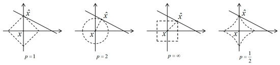
Figure 1.
Best approximation of a point in by a one-dimensional space using the LP norms for P = 1, 2, , and the LP quasinorm with .
Instead of minimizing the L0 norm in Equation (2), adopting the L1 norm and Equation (2) becomes:
The presence of the L1 term encourages small components of x to shrink to zero and promotes sparse solutions [12,14]. Theoretically, Equations (2) and (3) are approximately equivalent, but Equation (2) can obtain a sparser solution. Equation (3) is a convex optimal problem which can be solved by linear programming. Actually, there is a certain error between the reconstructed signal and the original signal. The residual value between them can be used to assess the approximation and accuracy of reconstructed signal, so Equation (3) can usually be expressed as:
and:
where and are real parameters with nonnegative values.
Equation (4) is a quadratically constrained linear program (QCLP) problem, whereas Equation (5) is a quadratic program (QP) [15]. Both Equations (4) and (5) are convex optimization problem, they easily reach the global optimal value, but they cannot guarantee the signal to be the sparsest. In addition, because L1 norm cannot be differentiated at zero, the L1 norm is non-analytic at zero and usually has a large amount of computation. For non-convex L0 norm optimization, the theoretical guarantee of the uniqueness of the global optimal solution is very weak, but the L0 norm non-convex reconstruction performs better than the L1 norm reconstruction at low sampling rates [16]. In order to utilize the advantages of the L0 norm and L1 norm reconstruction model, simultaneously reducing the number of measurements and the complexity of computation, the compromising minimum LP (0 < P < 1) norm algorithm is proposed in [17]. That is:
There are notably different properties of LP norms for different values of P. To illustrate this, in Figure 1 the unit sphere, i.e., , is induced by each of these norms in . We use a LP norm to measure the approximation error and our task is to find that minimizes [18]. As shown in Figure 1, to find the closest point in A to x by LP norm, we grow the LP sphere centered on x until it intersects with A. There will be the point that is closest to x for the corresponding LP norms. Through observation, we can know that a larger P tends to spread out the error more evenly among the two coefficients of two coordinate axes, while a smaller P leads to an error that is more unevenly distributed and tends to be sparser [18].
The above analysis is also applicable to higher dimensional situations, which plays an important role in CS theory. Reference [17] theoretically analyzes the feasibility of using LP norm instead of L0 norm. When the Restricted Isometric Property (RIP) condition [4,19] of the measurement matrix is weakened, the number of measurements needed for accurate reconstruction of the minimum LP norm method is greatly reduced compared with the minimum L1 norm method. Reference [20] further illustrates the necessary conditions of the parameter P and the constraint isometric constant (RIC) for the accurate reconstruction.
The Iterative Reweighted algorithm is proposed in [21,22] to solve the minimum LP norm problem. Some researchers use the method of dynamically shrinking parameter P (P asymptotically approximating to zero) to solve the minimum LP norm problem in the iterative process of the algorithm, which is described in detail in [23]. Other researchers fixed P to a value of 0 to 1, for example, in the L1/2 regularization algorithm [24]. Based on this idea of approximate L0 norm minimization, this paper proposes a new algorithm from L2 norm to approximate L0 norm by the method of gradient projection. The non-analytic problem of the L1 norm at zero is avoided, and the advantages of the convex optimization and non-convex optimization are also synthesized.
The remainder of this paper is organized as follows: in Section 2, we present a theoretical analysis of the new algorithm and introduce the basic algorithm framework. In Section 3, we introduce the specific algorithm process of L2 norm to approximate L0 norm using the method of gradient projection. In Section 4, simulation experiments are carried out to compare the new proposed algorithm with the traditional classic algorithms for the reconstruction of one-dimensional and two-dimensional signals. Finally, conclusions are drawn in Section 5.
2. Formulation from L2 Norm to Approximate L0 Norm
Our novel proposed algorithm approximates L0 norm from L2 norm based on our insight of the relationship between the L2 norm and L0 norm. In the algorithm, we do not set specific parameter P in LP norm. To approximate L0 norm, we first define an approximation function model. In the iterative process of new algorithm, the L0 norm is gradually approximated by changing the value of a modulation parameter in the function model. Thus, we can approximate the global optimal solution and the sparsest solution with greater probability and efficiency.
In Equation (1), x is the original signal, but generally the original signal maybe is not necessarily sparse. Therefore, the compressive sensing measurement and reconstruction of signal (Equations (1)−(6)) cannot perform well, and the original signal x must be transformed into some sparse domain i.e., , is a sparse transformation base, and is a sparse representation signal. Thus , , is called the sensing matrix.
To approximate L0 norm, an approximation function model is first defined as:
where is the ith element in the sparse signal s, and is the modulation parameter approximating the L0 norm, is the function value of the element in the sparse signal. The relation diagram of function and and is shown in Figure 2.
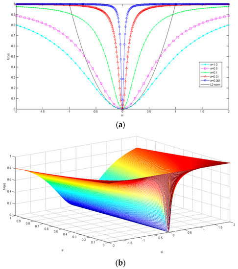
Figure 2.
(a) A 1D example of with different values. The L2 norm of the black solid line is included for comparison. (b) A 2D example surface plot of .
As shown in Figure 2, when is large, is approximately the L2 norm of signal s when is close to zero, as shown in the black solid line. When the value of decreases gradually, the gradually approaches the L0 norm of signal s, as shown in the middle curve of Figure 2a, that is:
That is, when is large, it is 1, and when is small, it is 0. For the summation of , we can get:
where n is the length of the sparse signal vector s. Obviously Equation (9) is equivalent to approximately calculating the number of non-zero items of sparse vector s, which is equivalent to get the L0 norm of sparse vector s when the sigma is very small, i.e., the optimization problem of the L0 norm can be nearly as . As shown in Figure 2, since the functional curve approximating L0 norm is smooth and derivable, it is also convenient to get the derivative of and the gradient of the objective function. Thus, minimizing the discontinuous function is transformed into minimizing the continuous function . Thus, Equation (2) is transformed into:
that is:
For the inverse problem of signal reconstruction, the prior of sparse representation is as a regularization term (the penalty function, ), so in order to obtain the optimal solution of the signal reconstruction, the constrained optimization of the approximation signal item should be considered. Based on the model Equation (10), Lagrangian method is applied to this constrained optimization problem, we add the residual of the reconstructed signal, and the compressed sensing signal reconstruction model with approximation L0 norm sparse representation is formed as:
In Equation (11) is the objective function we need to minimize. The goal of this algorithm is to seek the estimated value of sparse vector s which minimizes the objective function, where is the weight parameter used to adjust the weight of the sparse representation. Constant 1/2 of the reconstructed signal residual term is convenient to calculate the derivation of objective function. The sparse representation item in Equation (11) constrains the sparsity of signal s, and the reconstructed signal residual term is the minimal difference between the reconstructed signal measurement value and the actual measurement value, which can be considered as a global optimization for the whole signal. In order to find the minimum value of the target function , the parameter in is gradually reduced to make approximate to the L0 norm, so it is necessary to reduce the value of the parameter in the iterative process of the new proposed algorithm.
For general compress sensing signal reconstruction, the iterations of non-convex algorithm are usually prone to trapping at suboptimal local minima, for the reason that there are always combinatorial numbers of solutions for sparse signal. However, by applying in Equation (11), the problem of local minima can be implicitly avoided by solving it with a large initial beginning, such that the penalty function is initially nearly convex as (see Figure 2). As the iterations proceed and the details of the signal need to be reconstructed, the penalty function becomes less convex when has shrunk to the small, and is approximate to the L0 norm, but the risk of local minima and instability the solution falls into is ameliorated by the fact that the solution is already in the neighborhood of a desirable attraction basin of the global optimum. Thus, the implicit noise level (or modeling error between the reconstructed signal and the original signal) is now substantially less.
In this paper, the iterative gradient projection method is used to seek the minimum value of the objective function . The gradient of the objective function is obtained by deriving it with respect to s in (11):
Based on gradient projection, the basic algorithm framework of approximation minimum L0 norm algorithm is as Algorithm 1.
| Algorithm 1. Approximation Minimum L0 Norm. |
|
It is worth noting that, in the process of this algorithm, the is getting smaller and smaller with the iteration, and the decrease of makes the regular penalty term more and more close to the L0 norm. In order to reconstruct the original signal more accurately, we can make the weight of the error increase gradually, and then the regular penalty term is relatively reduced. Therefore, the value of the weight lambda can be adaptively adjusted in the iterative process according to the size of the error , which can be set into a descending sequence that is positively correlation with the value of the .
From Figure 2a,b, it is known that with the gradual decrease of , is increasingly approaching the smooth approximation of the L0 norm, which gradually constrains the sparsity of the reconstructed sparse signal and gradually approaches the global optimal solution in greater efficiency. Besides, subsequent iterations of the new algorithm begin to reflect the correct coarse shape, can be gradually reduced to allow the recovery of more detailed, fine structures. Thus the proposed algorithm reduces the complexity of the algorithm and improves the accuracy of the signal reconstruction. It is more conducive to signal reconstruction of compressed sensing. The next section will introduce the specific implementation of gradient projection in the new approximating L0 norm algorithm in detail.
3. The Gradient Projection Implementation in the Approximating L0 Norm Algorithm
In this section, we discuss GP (gradient projection) techniques for solving Equation (11). In order to minimize the objective function in Equation (11), as in [25], we split the variable into the positive and negative parts. Therefore, we introduce vector u and v to get the following substitution:
where and for all , is the length of the vector . is the positive-part operator defined as , so Equation (11) can be rewritten as the following bound-constrained quadratic program (BCQP):
where, . Further Equation (14) can be rewritten as:
where, , , , and:
In order to adjust the value of the sparsity term weight adaptively according to the error , we set to:
We can observe that the dimension of Equation (15) is twice that of the original problem (11): , while . However, this increase in dimension has only a minor impact on matrix operations, which can be performed more economically than its size suggests, by applying the particular structure (16) [15]. For a given , we have:
indicating that using only a single multiplication by can calculate the quantity. Since , in the same way that evaluation of also needs only one multiplication by .
In order to solve the objective function of Equation (15), we introduce the scalar parameter and update from iterate to iterate as follows:
For each iteration of , we search along the negative gradient direction , projecting onto the non negative orthant and conducting a backtracking line search until a sufficient decrease is attained in . (Bertsekas [26] refers to this strategy as “Armijo rule along the projection arc.”) There is an initial hypothesis that the technique would yield the exact smller value of along this direction if there are no new bounds to be encountered [15]. Specifically, the vector is defined as:
where , 2n is the number of elements in vector, and we initialize it by the following equation.
which can be computed by:
To prevent the value of from being too large or too small, we usually limit to an interval , where . That is, , the operator are defined as the middle value of three scalar arguments. When , . This method produces a more acceptable value of than the computed only by Equation (20) along the direction .
The implementation steps of the gradient projection algorithm approximating the L0 norm are shown in Algorithm 2.
| Algorithm 2. The Gradient Projection Approximating the L0 Norm. |
|
is the gradient of at for the kth iteration, and is the value of z at the kth iteration, is a constant of lower limit and the default value is 0.01. As the new proposed algorithm approximates to L0 norm minimization by the way of gradient projection, we refer to it as L0GP algorithm.
4. Experimental Analysis and Discussion
In the section, to verify the effectiveness of the proposed L0GP algorithm, simulation experiments are carried on by Matlab to reconstruct one-dimensional signal and two-dimensional image signals. For one-dimensional signal reconstruction experiments, we compare our algorithm L0GP with the classic L1-Regularized Least Squares (L1_LS) algorithm of L1 norm [11] such as Equation (3), and with the algorithm of minimum L2 norm, since the new proposed L0GP algorithm iteratively approximate L0 norm from L2 norm.
MSE, the mean square error is used to measure the reconstruction accuracy of one dimensional sparse signal. The definition is as follows:
where is the estimate of .
In the experiments, we take full account of a typical signal reconstruction of CS (similar to [11]), and our goal is to reconstruct an original sparse signal with a length of n and sparsity of k through a measured signal of a length of m, in which m < n. The signal are measured in space domain by matrix , which is a Gauss random matrix of size, and each element of the matrix is subject to a Gauss distribution with a mean value of 0 and a variance of 1/m. In this experiment, n = 4096, m = 1024, sparsity k = 220, which is the original sparse signal with a length of 4096, contains 220 non-zero values of a random distribution of +1, 0 or −1, and the observation y is generated by Equation (1). In the L0GP algorithm, the initial value of parameter is chosen as suggested in [11]
Notice that for , the unique minimum of Equation (3) is the zero vector [11,27], and parameters are set as . The values of these parameters are the relatively optimal results of a large number of experiments after we tried different parameters values. In the process of experiments adjusting parameters, we think the performance of our method is not particularly sensitive to these choices, as long as these parameters are in the certain interval. The minimum L0 norm solution is given by , that is, is the pseudo inverse solution of the undetermined system . The reconstruction results of one dimensional signal are shown in Figure 3.
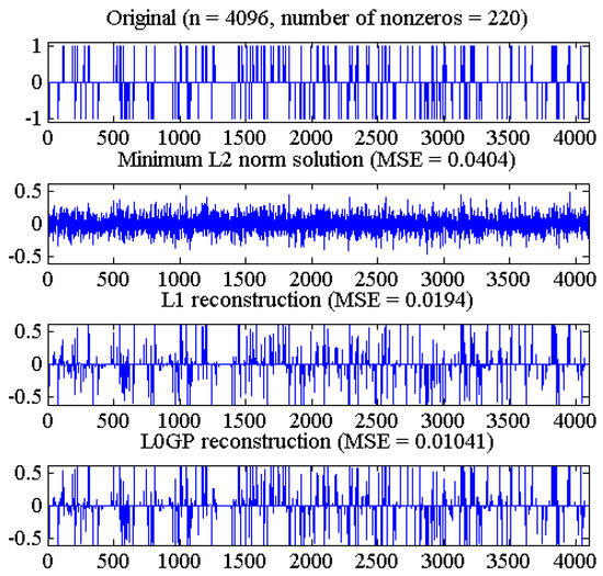
Figure 3.
From top to bottom: original signal, reconstruction obtained by the minimum L0 norm solution, L1_LS algorithm and the new proposed algorithm.
As shown in Figure 3, the L2 norm pseudo-inverse method can hardly recover the original signal, and the L1 norm algorithm is better than the pseudo-inverse method. The L0GP algorithm is superior to the L1 norm and L2 norm algorithms, and has smaller reconstruction error and higher reconstruction accuracy.
Since both the original sparse signal and the measurement matrix are randomly generated, the experiments’ results may be random. To assess these algorithms objectively, five experiments have been done for sparse signal reconstruction with the same sparsity, and then the average of their results is taken as the evaluation. This experiment takes n = 512, m = 128, and obtains the correlation between the reconstruction error of the sparse signal and the signal sparsity K among the three different methods, just as curve shown in the Figure 4.
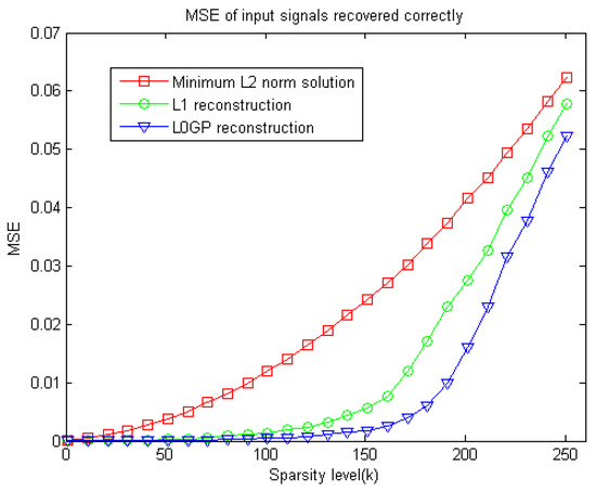
Figure 4.
MSE of sparse signal with different sparsity level recovered correctly by the three different reconstruction methods.
It is known from Figure 4, that the image reconstruction error of L0GP algorithm is less than the L1 norm algorithm and the L2 norm pseudo-inverse algorithm in the case of different sparsity. From the above two experiments, it can be seen that the new algorithm shows advantages from convex optimization to non-convex optimization and performs very well for the reconstruction of one dimensional sparse signals.
In order to further prove the good performance of L0GP algorithm, we furtherly do experiments on the reconstruction of non-sparse two-dimensional image signals. These experiments compared the new algorithm with other algorithms, such as Subspace Pursuit (SP) [28], Iterative Reweighted Least Squares (IRLS) [29], Orthogonal Matching Pursuit (OMP) [13], Regularized Orthogonal Matching Pursuit (ROMP) [30], Generalized Orthogonal Matching Pursuit (GOMP) [31], L1-Basis Pursuit (L1_BP) [12] and L1_LS [11].
The size of the experimental image is . If the two-dimensional image signal is simply arranged in a single column signal of one dimension, the length of the signal would be extremely large and also it will cost a lot of time for reconstruction. Therefore, our approach is to measure and sample the column signal () and the row signal () of the image in space domain respectively, which is equivalent to the reconstruction of the column signal or the row signal of the image, so the reconstruction time of the whole image also demonstrates the efficiency of the reconstruction algorithms. Since the two-dimensional image signal is a non-sparse signal in space domain, we need to transform it into the sparse representation domain by wavelet [17]. In this paper, we use discrete wavelet sparse transform (DWT) as the sparse basis, that is, the signal x are represented as in sparse domain, , is discrete wavelet basis.
In order to evaluate the accuracy of the reconstructed image, the peak signal to noise ratio (PSNR) and structural similarity (SSIM) are used as the evaluation index of the image, which are defined as follows:
where and are the mean values of x and respectively. , and are the variance or covariance values of x and respectively. and are the constants that maintain stability, , . L is the dynamic range of pixel values, , .
For the Mandrill image with a size of (n = ), we reconstruct the image by m times sampling of the image, m = 28900 (), and the sampling rate is about m/n = 1/9. The results of the experiment are shown in Figure 5.
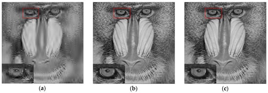
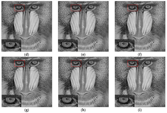
Figure 5.
Reconstruction results of different arithmetic of (a) SP, (b) IRLS, (c) OMP, (d) ROMP, (e) GOMP, (f) L1_BP, (g) L1_LS, (h) L0GP, (i) Original Mandrill image.
Then, PSNR, SSIM and the time of image reconstruction for the different algorithms are statistically obtained, and the results are shown in the following table.
From Figure 5 and Table 1, we can find that under the sampling rate of 1/9, compared with the suboptimal algorithm of the least norm and the greedy algorithm of the matching pursuit, the PSNR and SSIM of reconstructed image by the new proposed algorithm have been improved to a certain extent, and have higher image reconstruction accuracy. By zooming in the eye area of the mandrill marked by red box, it can be seen that the details of the reconstructed image become clearer and the picture quality is better, and the sharpness of image edge is well enhanced and the noise becomes less.

Table 1.
The quantitative results of different algorithms.
Because the time of the image reconstruction of the greedy algorithm of the matching pursuit class depends on the number of iterations or the terminating conditions, although the image reconstruction time of ROMP algorithm is very short, the image reconstruction accuracy of ROMP is much worse than that of L0GP. Moreover, when the number of iterations reaches a certain number, the image reconstruction accuracy of ROMP will not increase obviously with the number of iterations, instead, it will consume a lot of time and computation. Owning to fact that the L0GP can quickly approximate the global optimal solution with bigger probability, the reconstruction time is greatly reduced much more than the traditional iterative least square algorithm (IRLS) and the L1 norm algorithm. Comparing L0GP with the traditional iterative least square algorithm (IRLS) and L1 norm algorithm, the reconstruction time is greatly shortened and the image reconstruction accuracy is improved, so the advantage of this algorithm is evident.
In order to prove the validity and generality of the L0GP algorithm for various image reconstruction, we choose six representative images, including nature scenes, persons, animals, detailed and texture images, as shown in Figure 6. At the same sampling rate of 1/9, these images were reconstructed. The quantitative results of the experiment are shown in Table 2.
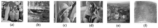
Figure 6.
Different representative images of (a) Peppers, (b) Bridge, (c) Lena, (d) Barbara, (e) Goldhill, (f) Fingerprint.
Table 2.
The quantitative results (PSNR/SSIM) of different algorithms for the different types of images.
Analyzing the data in Table 2, the proposed algorithm has a good performance in the reconstruction of various types of images, and has a good advantage over the other seven algorithms. It shows that the new algorithm has a strong generality and adaptability for all kinds of images.
For the Fingerprint image with a size of (n = ), we increase the number of sampling on the image and do the simulation experiment again. We reconstruct the image by m times sampling of image, m = 65536 (), i.e., the sampling rate is about m/n = 1/4. The results of the experiment are shown in Figure 7.
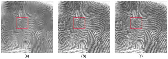
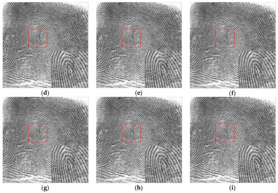
Figure 7.
Reconstruction results of different algorithms of (a) SP, (b) IRLS, (c) OMP, (d) ROMP, (e) GOMP, (f) L1_BP, (g) L1_LS, (h) L0GP, (i) Original Fingerprint image.
As shown in Figure 7 and Table 3, the texture and details of the Fingerprint image are well reconstructed. Clearly, the proposed algorithm show better performance at reconstructing fine structures. Moreover, the blur is obviously suppressed, meanwhile the new algorithm reconstructs more rich information than the others, and the reconstructed image has the highest PSNR and SSIM in the quantitative assessment indexes.
Table 3.
The quantitative results of different arithmetics.
For the large amount of data like image and the reconstruction of high sampling rate signal, the greedy algorithm of the OMP class has weak theoretical guarantee. From the data statistics above Figure 7 and Table 3, the accuracy and time of the reconstruction cannot reach the ideal at the same time, and the accurate reconstruction of the signal has some randomness. Therefore, the greedy algorithm for OMP class often considers the time cost on the basis of satisfying the reconstruction accuracy, and takes a compromise between the reconstruction time and the reconstruction accuracy. Similarly, when the sampling rate is 1/4, different types of images are reconstructed, and statistical data are obtained as shown in Table 4.
Table 4.
The quantitative results (PSNR/SSIM) of different algorithms for the different types of images.
Based on the data statistics of the above experiments, with increasing signal sampling rate, more information of the original signal is obtained from sampling, so the advantages of the new proposed algorithm have been weakened slightly. Although the performance of the new proposed L0GP algorithm is not the best in the reconstruction time, the reconstruction time is also very short and the accuracy of the reconstructed signal is the highest among the eight algorithms. The experimental simulation results also further verify the effectiveness of the algorithm theory analysis in Section 2 and Section 3.
5. Conclusions
In this paper, a gradient projection algorithm approximating the minimum L0 norm from the L2 norm is proposed to solve the optimization problem of sparse signal reconstruction. This new algorithm integrates the characteristics of both convex optimization and non-convex optimization algorithm, making the algorithm approximate the global optimal sparse solution with higher probability and higher efficiency in the iterative process. The simulations are carried out on sparse signal reconstructions of one-dimensional signal and two-dimensional no sparse signal. Compared with the convex optimization algorithm of the minimum norm and the greedy algorithm of the matching tracking, the new proposed algorithm performs better in the precision and speed of reconstructing signal. Especially under the low sampling rate of sparse signal, the performance of L0GP is much outstanding. As a result, the required number of measurements for sparse signal of compressed sensing would be less and the speed of compressed sensing can be accelerated greatly.
Author Contributions
Z.W. made significant contributions to this study regarding conception, methodology and analysis, and writing the manuscript. J.Z. contributed much to the research through his general guidance and advice, and optimized the paper. Z.X. made research plans and managed the study project. Y.H. and Y.L. gave much advices and help on experimental simulation. X.F. contributed to the revision of the manuscript.
Funding
This research received no external funding.
Acknowledgments
We would like to gratefully acknowledge Wei Yang for technical support.
Conflicts of Interest
The authors declare that there are no conflicts of interests regarding the publication of this paper.
References
- Donoho, D.L. Compressed sensing. IEEE Trans. Inf. Theory 2006, 52, 1289–1306. [Google Scholar] [CrossRef]
- Boche, H.; Calderbank, R.; Kutyniok, G.; Vybiral, J. Compressed Sensing and Its Applications; Springer: Berlin/Heidelberg, Germany, 2015. [Google Scholar]
- Candès, E.J.; Romberg, J.; Tao, T. Robust uncertainty principles: Exact signal reconstruction from highly incomplete frequency information. IEEE Trans. Inf. Theory 2006, 52, 489–509. [Google Scholar] [CrossRef]
- Candès, E.J.; Tao, T. Near-optimal signal recovery from random projections: Universal encoding strategies. IEEE Trans. Inf. Theory 2006, 52, 5406–5425. [Google Scholar] [CrossRef]
- Candès, E.J.; Romberg, J.K. Practical signal recovery from random projections. In Computational Imaging III; SPIE: Bellingham, WA, USA, 2004; p. 5674. [Google Scholar]
- Baraniuk, R.G. Compressive sensing. IEEE Signal Process. Mag. 2007, 24, 118–121. [Google Scholar] [CrossRef]
- Chen, C.; Tramel, E.W.; Fowler, J.E. Compressed-sensing recovery of images and video using multihypothesis predictions. In Proceedings of the 2011 Conference Record of the Forty Fifth Asilomar Conference on Signals, Systems and Computers (ASILOMAR), Pacific Grove, CA, USA, 6–9 November 2011. [Google Scholar]
- Zhang, J.; Yin, Y.; Yin, Y. Adaptive compressed sensing for wireless image sensor networks. Multimed. Tools Appl. 2017, 76, 1–16. [Google Scholar] [CrossRef]
- Candès, E.; Romberg, J.; Tao, T. Stable signal recovery from incomplete and inaccurate measurements. Commun. Pure Appl. Math. 2006, 59, 1207–1223. [Google Scholar] [CrossRef]
- Donoho, D.; Tsaig, Y. Extensions of compressed sensing. Signal Process. 2006, 86, 533–548. [Google Scholar]
- Kim, S.-J.; Koh, K.; Lustig, M.; Boyd, S.; Gorinevsky, D. A Interior-Point Method for Large-Scale l1-Regularized Least Square. IEEE J. Sel. Top. Signal Process. 2007, 1, 606–617. [Google Scholar] [CrossRef]
- Chen, S.S.; Donoho, D.L.; Saunders, M.A. Atomic decomposition by basis pursuit. SIAM Rev. 2001, 43, 129–159. [Google Scholar] [CrossRef]
- Tropp, J.A.; Gilbert, A.C. Signal Recovery from Random Measurements via Orthogonal Matching Pursuit. IEEE Trans. Inf. Theory 2007, 53, 4655–4666. [Google Scholar] [CrossRef]
- Tibshirani, R. Regression shrinkage and selection via the lasso. J. R. Statist. Soc. B 1996, 58, 267–288. [Google Scholar]
- Figueiredo, M.A.T.; Nowak, R.D.; Wright, S.J. Gradient Projection for Sparse Reconstruction: Application to Compressed Sensing and Other Inverse Problems. IEEE J. Sel. Top. Signal Process. 2008, 1, 586–597. [Google Scholar] [CrossRef]
- TRzasko, J.; Manduca, A. Relaxed conditions for sparse signal recovery with general concave priors. IEEE Trans. Signal Process. 2009, 57, 4347–4354. [Google Scholar] [CrossRef]
- Wang, Q.; Li, D.; Shen, Y. Intelligent nonconvex compressive sensing using prior information for image reconstruction by sparse representation. Neurocomputing 2017, 224, 71–81. [Google Scholar] [CrossRef]
- Eldar, Y.C.; Kutyniok, G. Compressed Sensing: Theory and Applications, 1st ed.; Cambridge University Press: Cambridge, UK, 2012; ISBN-10 1107005582. [Google Scholar]
- Candès, E.; Romberg, J. Sparsity and incoherence in compressive sampling. Inverse Probl. 2007, 23, 969–985. [Google Scholar] [CrossRef]
- Davies, M.E.; Gribonval, R. Restricted isometry constants where Lp sparse recovery can fail for 0 < p <= 1. IEEE Trans. Inf. Theory 2009, 55, 2203–2214. [Google Scholar] [CrossRef]
- Needell, D.; Tropp, J.A. Cosamp: Iterative signal recovery from incomplete and inaccurate samples. Commun. ACM 2010, 53, 93–100. [Google Scholar] [CrossRef]
- Daubechies, I.; DeVore, R.; Fornasier, M. Iteratively reweighted least squares minimization for sparse recovery. Commun. Pure Appl. Math. 2010, 63, 1–38. [Google Scholar] [CrossRef]
- Liu, Z.; Zhen, X. Variable-p iteratively weighted algorithm for image reconstruction. In Artificial Intelligence and Computational Intelligence; Springer: Berlin/Heidelberg, Germany, 2011; pp. 344–351. [Google Scholar]
- Xu, Z.; Chang, X.; Xu, F. L1/2 regularization: A thresholding representation theory and a fast solver. IEEE Trans. Neural Netw. Learn. Syst. 2012, 23, 1013–1027. [Google Scholar] [PubMed]
- Fuchs, J.J. Multipath time-delay detection and estimation. IEEE Trans. Signal Process. 1999, 47, 237–243. [Google Scholar] [CrossRef]
- Bertsekas, D.P. Nonlinear Programming, 2nd ed.; Athena Scientific: Boston, MA, USA, 1999. [Google Scholar]
- Fuchs, J.J. More on sparse representations in arbitrary bases. IEEE Trans. Inf. Theory 2004, 50, 1341–1344. [Google Scholar] [CrossRef]
- Dai, W.; Milenkovic, O. Subspace pursuit for compressive sensing signal reconstruction. IEEE Trans. Inf. Theory 2009, 55, 2230–2249. [Google Scholar] [CrossRef]
- Chartrand, R.; Yin, W. Iteratively Reweighted Algorithms for Compressive Sensing; CAAM Technical Reports [719]; Rice University: Houston, TA, USA, 2008. [Google Scholar]
- Needell, D.; Vershynin, R. Signal recovery from incomplete and inaccurate measurements via regularized orthogonal matching pursuit. IEEE J. Sel. Top. Signal Process. 2010, 4, 310–316. [Google Scholar] [CrossRef]
- Wang, J.; Kwon, S.; Shim, B. Generalized orthogonal matching pursuit. IEEE Trans. Signal Process. 2012, 60, 6202–6216. [Google Scholar] [CrossRef]
© 2018 by the authors. Licensee MDPI, Basel, Switzerland. This article is an open access article distributed under the terms and conditions of the Creative Commons Attribution (CC BY) license (http://creativecommons.org/licenses/by/4.0/).