A New Localization System for Indoor Service Robots in Low Luminance and Slippery Indoor Environment Using Afocal Optical Flow Sensor Based Sensor Fusion


Abstract
:1. Introduction
2. Related Works
2.1. Slippage Detection Methods
2.2. Image Enhancement under Low Luminance
2.3. Identifying Indoor Structure Using a Single Image
3. Proposed Methods
| Algorithm 1. Robot localization algorithm | |
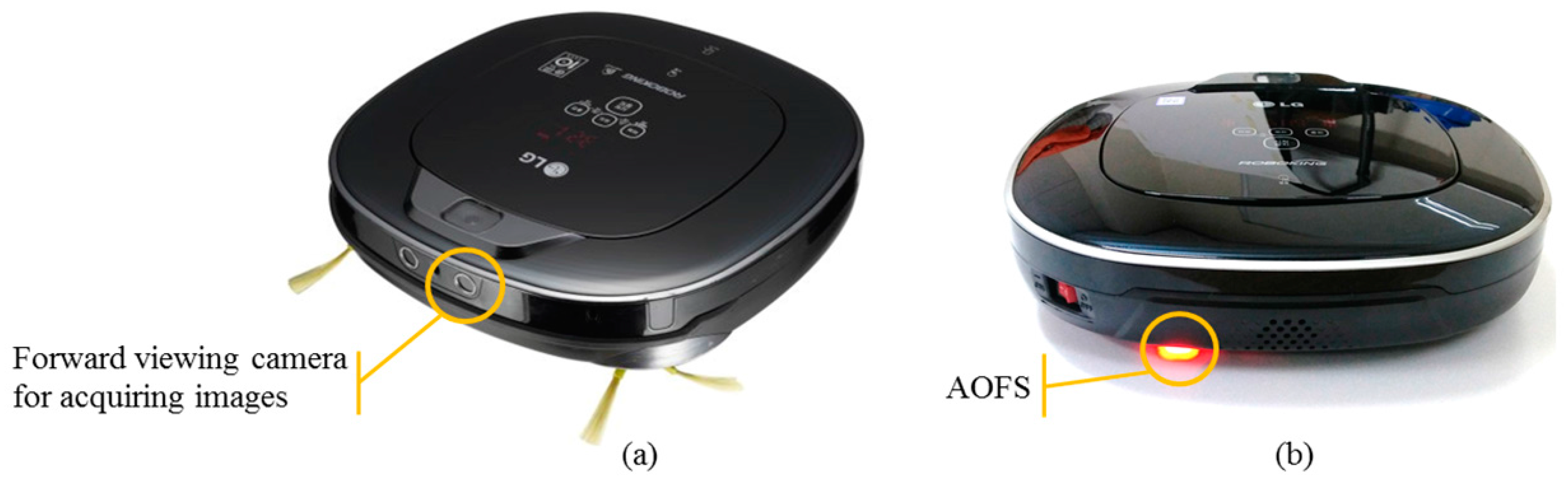
| Input: | AOFS, wheel encoders, a gyroscope, and a foward viewing image |
| Output: | Optimized robot pose trajectory |
| 1: | For every samples do |
| 2: | generate odometry data with the AOFS, wheel encoders, and the gyroscope |
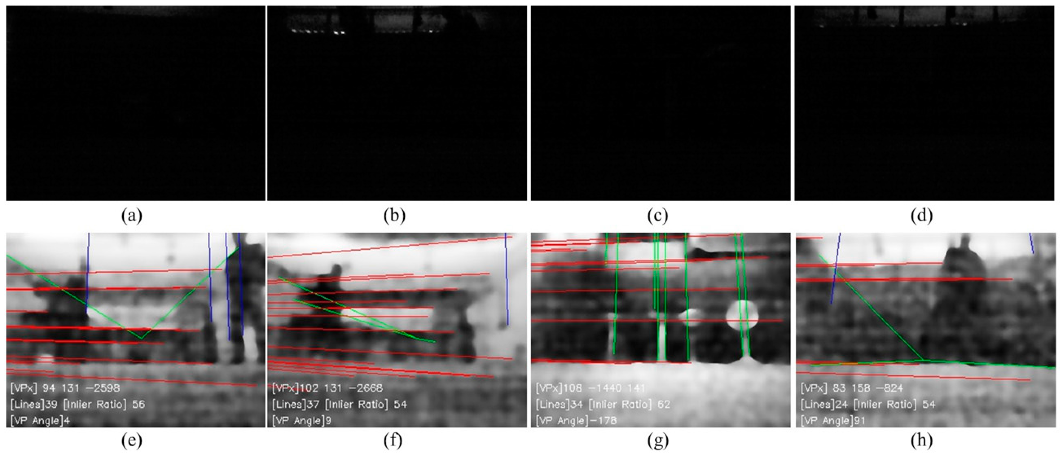
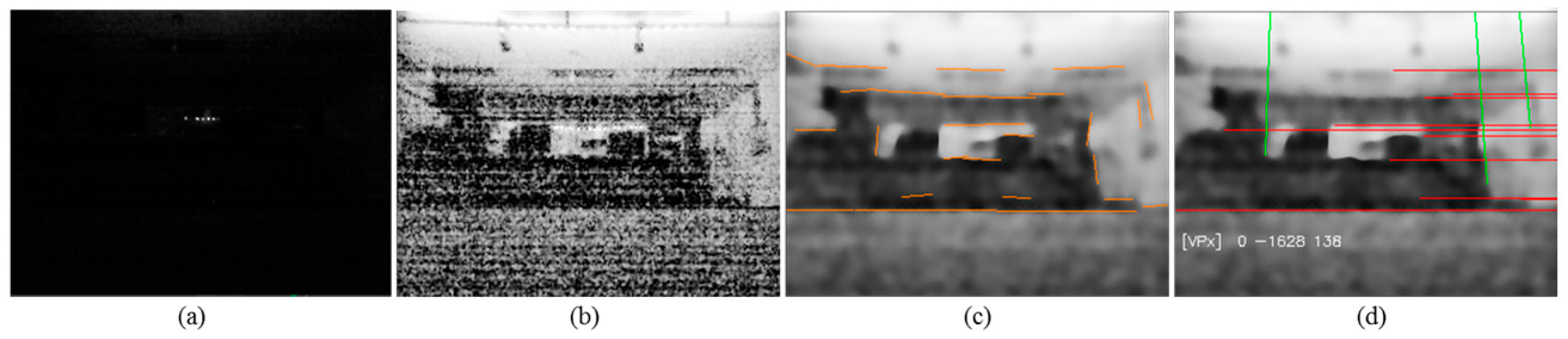
| 3: | apply rolling guidance filter after histogram equalization to the image |
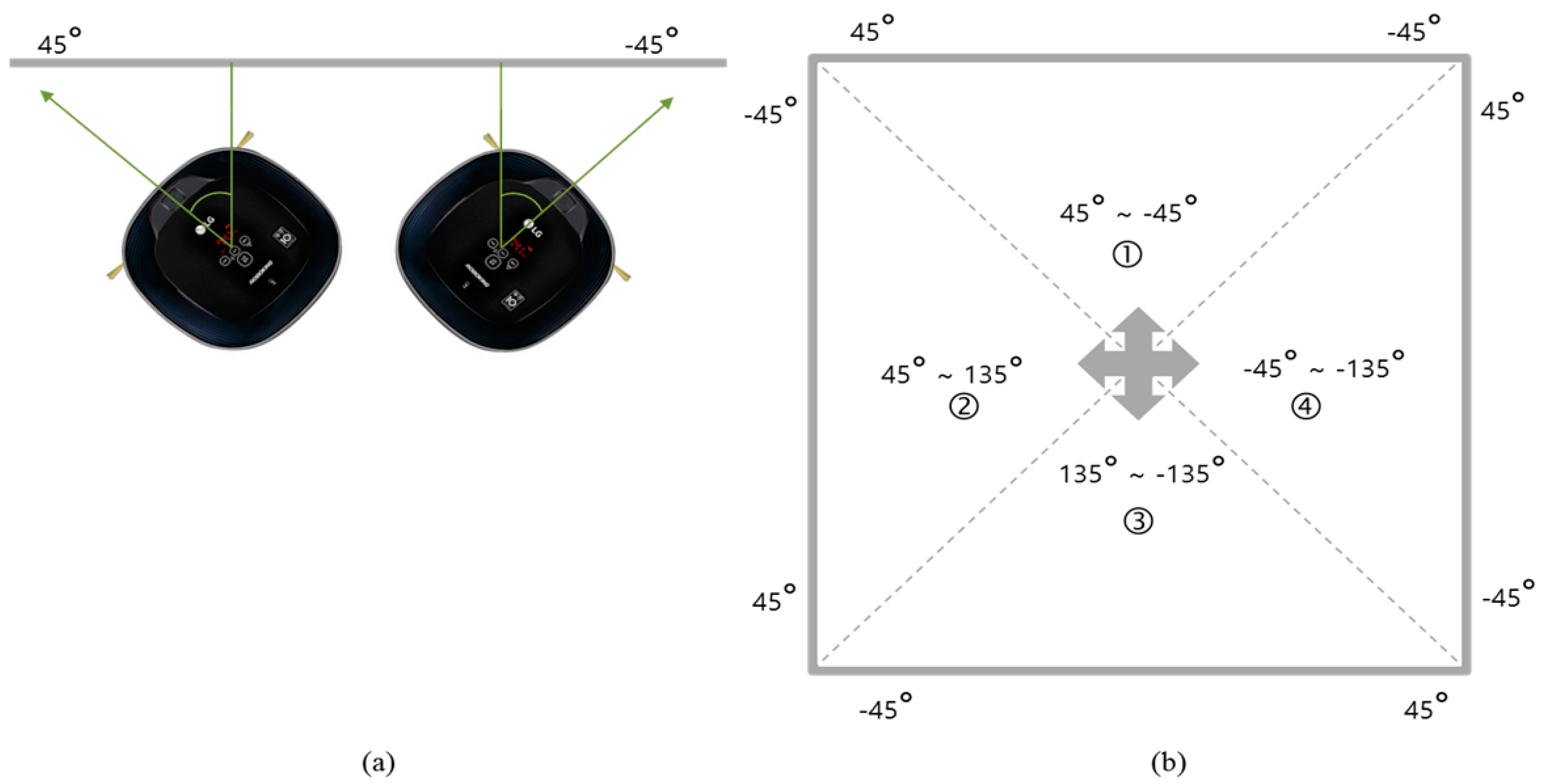
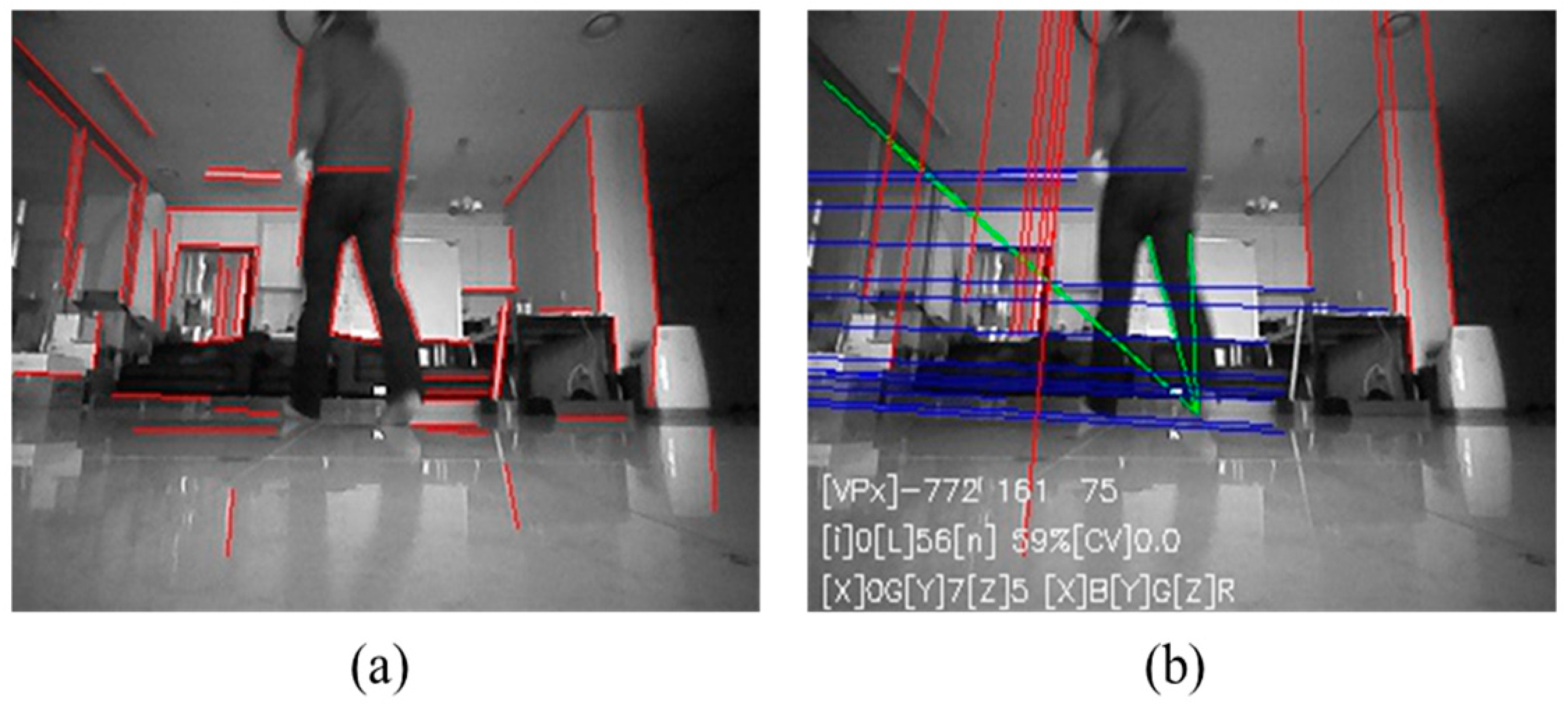
| 4: | extract vanishing points from the image |
| 5: | estimate robot azimuth from the vanishing points |
| 6: | optimization robot pose trajectory using the Lebenberg–Marquard algorithm |
| 7: | return the optimized robot pose trajectory |
| 8: | end For |
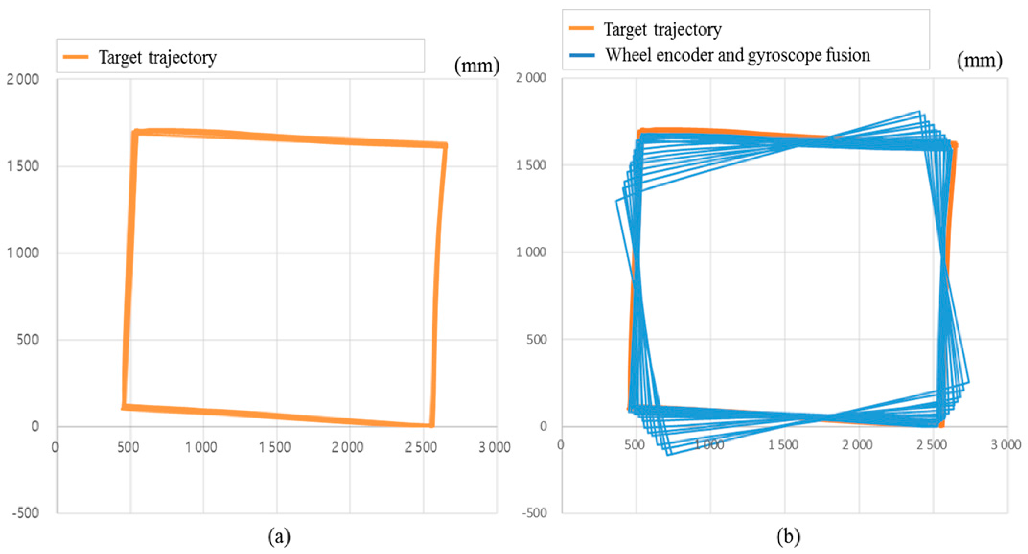
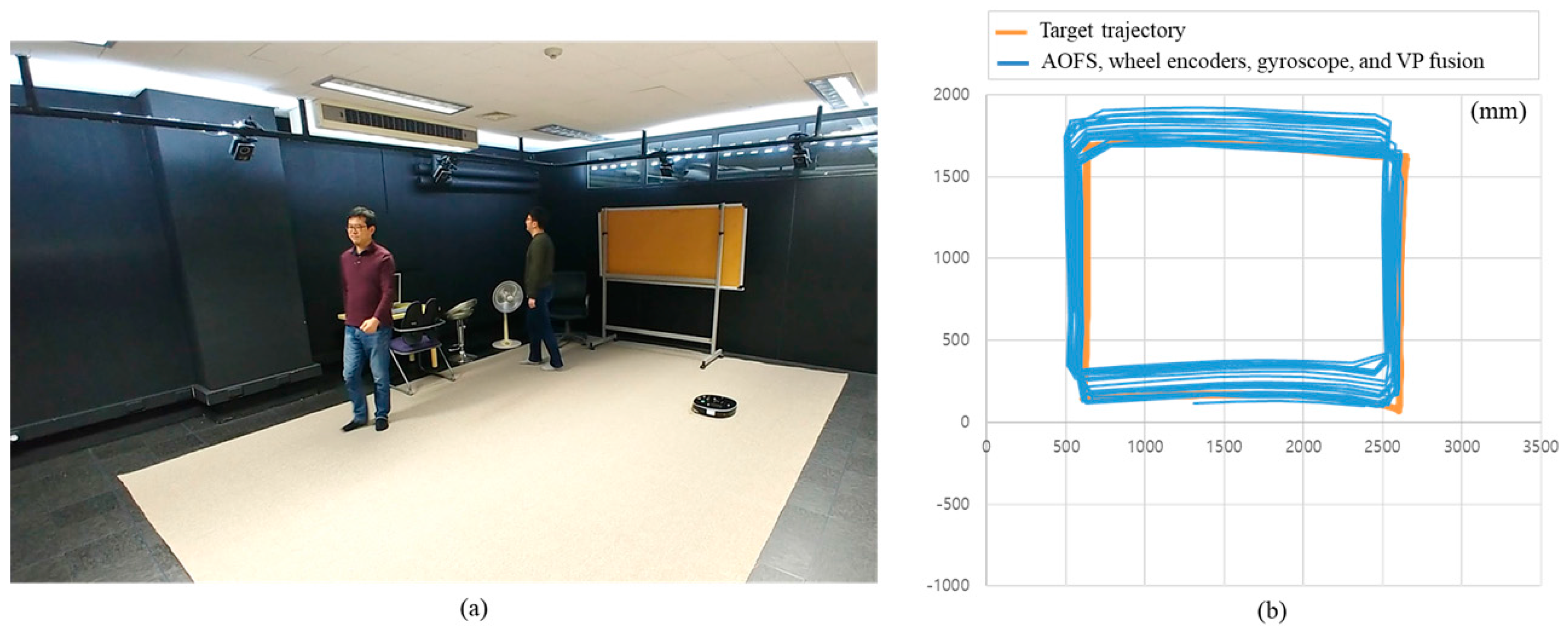
4. Experiments
5. Discussion
6. Conclusions
Acknowledgments
Author Contributions
Conflicts of Interest
References
- Passafiume, M.; Maddio, S.; Cidronali, A. An improved approach for RSSI-based only calibration-free real-time indoor localization on IEEE 802.11 and 802.15.4 wireless networks. Sensors 2017, 17. [Google Scholar] [CrossRef] [PubMed]
- Showcase, R.; Biswas, J.; Veloso, M.M.; Veloso, M. WiFi Localization and Navigation for Autonomous Indoor Mobile Robots. In Proceedings of the IEEE International Conference on Robotics and Automations, Anchorage, AK, USA, 3–8 May 2010; pp. 4379–4384. [Google Scholar]
- Alarifi, A.; Al-Salman, A.; Alsaleh, M.; Alnafessah, A.; Al-Hadhrami, S.; Al-Ammar, M.; Al-Khalifa, H. Ultra Wideband Indoor Positioning Technologies: Analysis and Recent Advances. Sensors 2016, 16, 707. [Google Scholar] [CrossRef] [PubMed]
- Park, J.; Cho, Y.K.; Martinez, D. A BIM and UWB integrated Mobile Robot Navigation System for Indoor Position Tracking Applications. J. Constr. Eng. Proj. Manag. 2016, 6, 30–39. [Google Scholar] [CrossRef]
- Shim, J.H.; Cho, Y.I. A mobile robot localization via indoor fixed remote surveillance cameras. Sensors 2016, 16, 195. [Google Scholar] [CrossRef] [PubMed]
- Haehnel, D.; Burgard, W.; Fox, D.; Fishkin, K.; Philipose, M. Mapping and Localization with RFID Technology. In Proceedings of the IEEE International Conference on Robotics and Automations, New Orleans, LA, USA, 26 April–1 May 2004; pp. 1015–1020. [Google Scholar]
- Mi, J.; Takahashi, Y. An design of HF-band RFID system with multiple readers and passive tags for indoor mobile robot self-localization. Sensors 2016, 16, 1200. [Google Scholar] [CrossRef] [PubMed]
- Royer, E.; Lhuillier, M.; Dhome, M.; Lavest, J.-M. Monocular Vision for Mobile Robot Localization and Autonomous Navigation. Int. J. Comput. Vis. 2007, 74, 237–260. [Google Scholar] [CrossRef]
- Di, K.; Zhao, Q.; Wan, W.; Wang, Y.; Gao, Y. RGB-D SLAM based on extended bundle adjustment with 2D and 3D information. Sensors 2016, 16. [Google Scholar] [CrossRef] [PubMed]
- Lingemann, K.; Nüchter, A.; Hertzberg, J.; Surmann, H. High-speed laser localization for mobile robots. Rob. Auton. Syst. 2005, 51, 275–296. [Google Scholar] [CrossRef]
- Jung, J.; Yoon, S.; Ju, S.; Heo, J. Development of kinematic 3D laser scanning system for indoor mapping and as-built BIM using constrained SLAM. Sensors 2015, 15, 26430–26456. [Google Scholar] [CrossRef] [PubMed]
- Mur-Artal, R.; Montiel, J.; Tardos, J. ORB-SLAM: A Versatile and Accurate Monocular SLAM System. IEEE Trans. Rob. 2015, 31, 1147–1163. [Google Scholar] [CrossRef]
- Engel, J.; Schöps, T.; Cremers, D.; Schöps, T.; Cremers, D. LSD-SLAM: Large-Scale Direct monocular SLAM. In Proceedings of the European Conference on Computer Vision, Zurich, Switzerland, 6–12 September 2014; pp. 834–849. [Google Scholar]
- Reina, G.; Ojeda, L.; Milella, A.; Borenstein, J.; Member, S. Wheel slippage and sinkage detection for planetary rovers. IEEE/ASME Trans. Mechatron. 2006, 11, 185–195. [Google Scholar] [CrossRef]
- Cooney, J.A.; Xu, W.L.; Bright, G. Visual dead-reckoning for motion control of a Mecanum-wheeled mobile robot. Mechatronics 2004, 14, 623–637. [Google Scholar] [CrossRef]
- Seyr, M.; Jakubek, S. Proprioceptive navigation, slip estimation and slip control for autonomous wheeled mobile robots. In Proceedings of the IEEE Conference on Robotics, Automation and Mechatronics, Bangkok, Thailand, 1–3 June 2006; pp. 1–6. [Google Scholar]
- Batista, P.; Silvestre, C.; Oliveira, P.; Cardeira, B. Accelerometer calibration and dynamic bias and gravity estimation: Analysis, design, and experimental evaluation. IEEE Trans. Control Syst. Technol. 2011, 19, 1128–1137. [Google Scholar] [CrossRef]
- Jackson, J.D.; Callahan, D.W.; Marstrander, J. A rationale for the use of optical mice chips for economic and accurate vehicle tracking. In Proceedings of the IEEE International Conference on Automation Science and Engineering, Scottsdale, AZ, USA, 22–25 September 2007; pp. 939–944. [Google Scholar]
- McCarthy, C.; Barnes, N. Performance of optical flow techniques for indoor navigation with a mobile robot. In Proceedings of the IEEE International Conference on Robotics and Automation, New Orleans, LA, USA, 26 April–1 May 2004; pp. 5093–5098. [Google Scholar]
- Palacin, J.; Valgañon, I.; Pernia, R. The optical mouse for indoor mobile robot odometry measurement. Sens. Actuators A 2006, 126, 141–147. [Google Scholar] [CrossRef]
- Lee, S.Y.; Song, J.B. Robust mobile robot localization using optical flow sensors and encoders. In Proceedings of the IEEE International Conference on Robotics and Automation, New Orleans, LA, USA, 26 April–1 May 2004; pp. 1039–1044. [Google Scholar]
- Avago. ADNS-3080 and ADNS-3088 High Performance Optical Sensor. Available online: http://www.alldatasheet.com (accessed on 28 November 2017).
- Minoni, U.; Signorini, A. Low-cost optical motion sensors: An experimental characterization. Sens. Actuators A 2006, 128, 402–408. [Google Scholar] [CrossRef]
- Kim, S.; Lee, S. Robust velocity estimation of an omnidirectional mobile robot using a polygonal array of optical mice. In Proceedings of the IEEE International Conference on Information and Automation, Changsha, China, 20–23 June 2008; pp. 713–721. [Google Scholar]
- Dahmen, H.; Mallot, H.A. Odometry for ground moving agents by optic flow recorded with optical mouse chips. Sensors 2014, 14, 21045–21064. [Google Scholar] [CrossRef] [PubMed]
- Ross, R.; Devlin, J.; Wang, S. Toward refocused optical mouse sensors for outdoor optical flow odometry. IEEE Sens. J. 2012, 12, 1925–1932. [Google Scholar] [CrossRef]
- Dille, M.; Grocholsky, B.; Singh, S. Outdoor Downward-facing Optical Flow Odometry with Commodity Sensors. Field Serv. Robot. 2009, 1–10. [Google Scholar] [CrossRef]
- Hyun, D.J.; Yang, H.S.; Park, H.R.; Park, H.S. Differential optical navigation sensor for mobile robots. Sens. Actuators A 2009, 156, 296–301. [Google Scholar] [CrossRef]
- Yi, D.H.; Lee, T.J.; Cho, D.I. Afocal optical flow sensor for reducing vertical height sensitivity in indoor robot localization and navigation. Sensors 2015, 15, 11208–11221. [Google Scholar] [CrossRef] [PubMed]
- Pizer, S.M.; Amburn, E.P.; Austin, J.D.; Cromartie, R.; Geselowitz, A.; Greer, T.; Ter Haar Romeny, B.; Zimmerman, J.B.; Zuiderveld, K. Adaptive Histogram Equalization and Its Variations. Comput. Vis. Graph. Image Process. 1987, 39, 355–368. [Google Scholar] [CrossRef]
- Maddern, W.; Stewart, A.D.; McManus, C.; Upcroft, B.; Churchill, W.; Newman, P. Illumination Invariant Imaging: Applications in Robust Vision-based Localisation, Mapping and Classification for Autonomous Vehicles. In Proceedings of the IEEE International Conference on Robotics and Automation, Hong Kong, China, 31 May–7 June 2014; p. 3. [Google Scholar]
- Park, C.; Song, J.B. Illumination Change Compensation and Extraction of Corner Feature Orientation for Upward-Looking Camera-Based SLAM. In Proceedings of the 12th International Conference on Ubiquitous Robots and Ambient Intelligence, Goyang, Korea, 28–30 October 2015; pp. 224–227. [Google Scholar]
- Zuiderveld, K. Graphics Gems IV. In Contrast Limited Adaptive Histogram Equalization; Heckbert, P.S., Ed.; Academic Press: Cambridge, MA, USA, 1994; Chapter VIII.5; pp. 474–485. ISBN 0-12-336155-9. [Google Scholar]
- Land, E.H.; McCann, J.J. Lightness and Retinex Theory. J. Opt. Soc. Am. 1971, 61, 1–11. [Google Scholar] [CrossRef] [PubMed]
- Rahman, Z.; Jobson, D.J.; Woodell, G.A. Retinex processing for automatic image enhancement. J. Electron. Imag. 2004, 13. [Google Scholar] [CrossRef]
- Chang, H.C.; Huang, S.H.; Lai, S.H. Using line consistency to estimate 3D indoor Manhattan scene layout from a single image. In Proceedings of the IEEE International Conference on Image Processing, Quebec City, QC, Canada, 27–30 September 2015; pp. 4723–4727. [Google Scholar]
- Zhang, L.; Lu, H.; Hu, X.; Koch, R. Vanishing Point Estimation and Line Classification in a Manhattan World. Int. J. Comput. Vis. 2016, 117, 111–130. [Google Scholar] [CrossRef]
- Flint, A.; Murray, D.; Reid, I. Manhattan scene understanding using monocular, stereo, and 3D features. In Proceedings of the IEEE International Conference on Computer Vision, Barcelona, Spain, 6–13 November 2011; pp. 2228–2235. [Google Scholar]
- Jia, H.; Li, S. Estimating the structure of rooms from a single fisheye image. In Proceedings of the 2nd IAPR Asian Conference on Pattern Recognition, Naha, Japan, 5–8 November 2013; pp. 818–822. [Google Scholar]
- Schwing, A.G.; Fidler, S.; Pollefeys, M.; Urtasun, R. Box in the box: Joint 3D layout and object reasoning from single images. In Proceedings of the IEEE International Conference on Computer Vision, Sydney, NSW, Australia, 1–8 December 2013; pp. 353–360. [Google Scholar]
- Zhang, Q.; Shen, X.; Xu, L.; Jia, J. Rolling guidance filter. In Proceedings of the 13th European Conference, Zurich, Switzerland, 6–12 September 2014; pp. 815–830. [Google Scholar] [CrossRef]


© 2018 by the authors. Licensee MDPI, Basel, Switzerland. This article is an open access article distributed under the terms and conditions of the Creative Commons Attribution (CC BY) license (http://creativecommons.org/licenses/by/4.0/).
Share and Cite
Yi, D.-H.; Lee, T.-J.; Cho, D.-I.“. A New Localization System for Indoor Service Robots in Low Luminance and Slippery Indoor Environment Using Afocal Optical Flow Sensor Based Sensor Fusion. Sensors 2018, 18, 171. https://doi.org/10.3390/s18010171
Yi D-H, Lee T-J, Cho D-I“. A New Localization System for Indoor Service Robots in Low Luminance and Slippery Indoor Environment Using Afocal Optical Flow Sensor Based Sensor Fusion. Sensors. 2018; 18(1):171. https://doi.org/10.3390/s18010171
Chicago/Turabian StyleYi, Dong-Hoon, Tae-Jae Lee, and Dong-Il “Dan” Cho. 2018. "A New Localization System for Indoor Service Robots in Low Luminance and Slippery Indoor Environment Using Afocal Optical Flow Sensor Based Sensor Fusion" Sensors 18, no. 1: 171. https://doi.org/10.3390/s18010171
APA StyleYi, D.-H., Lee, T.-J., & Cho, D.-I. “. (2018). A New Localization System for Indoor Service Robots in Low Luminance and Slippery Indoor Environment Using Afocal Optical Flow Sensor Based Sensor Fusion. Sensors, 18(1), 171. https://doi.org/10.3390/s18010171