Multi-Frame Super-Resolution of Gaofen-4 Remote Sensing Images


Abstract
1. Introduction
2. Materials and Methods
2.1. Observation Model
2.2. Image Registration
| Algorithm 1. Image registration algorithm. | |
| 1 | Input: LR images . |
| 2 | Output: Geometric and photometric parameters. |
| 3 | Select one image as the reference image, and detect its SURF features. |
| 4 | for , do |
| 5 | Detect SURF features of the LR image . |
| 6 | Match features of and , then estimate geometric parameters based on RANSAC. |
| 7 | do |
| 8 | Estimate photometric parameters using conjugate gradient method for fixed geometric parameters . |
| 9 | Estimate geometric parameters using the Marquardt-Levenberg method for fixed photometric parameters . |
| 10 | until and do not change anymore. |
| 11 | endfor |
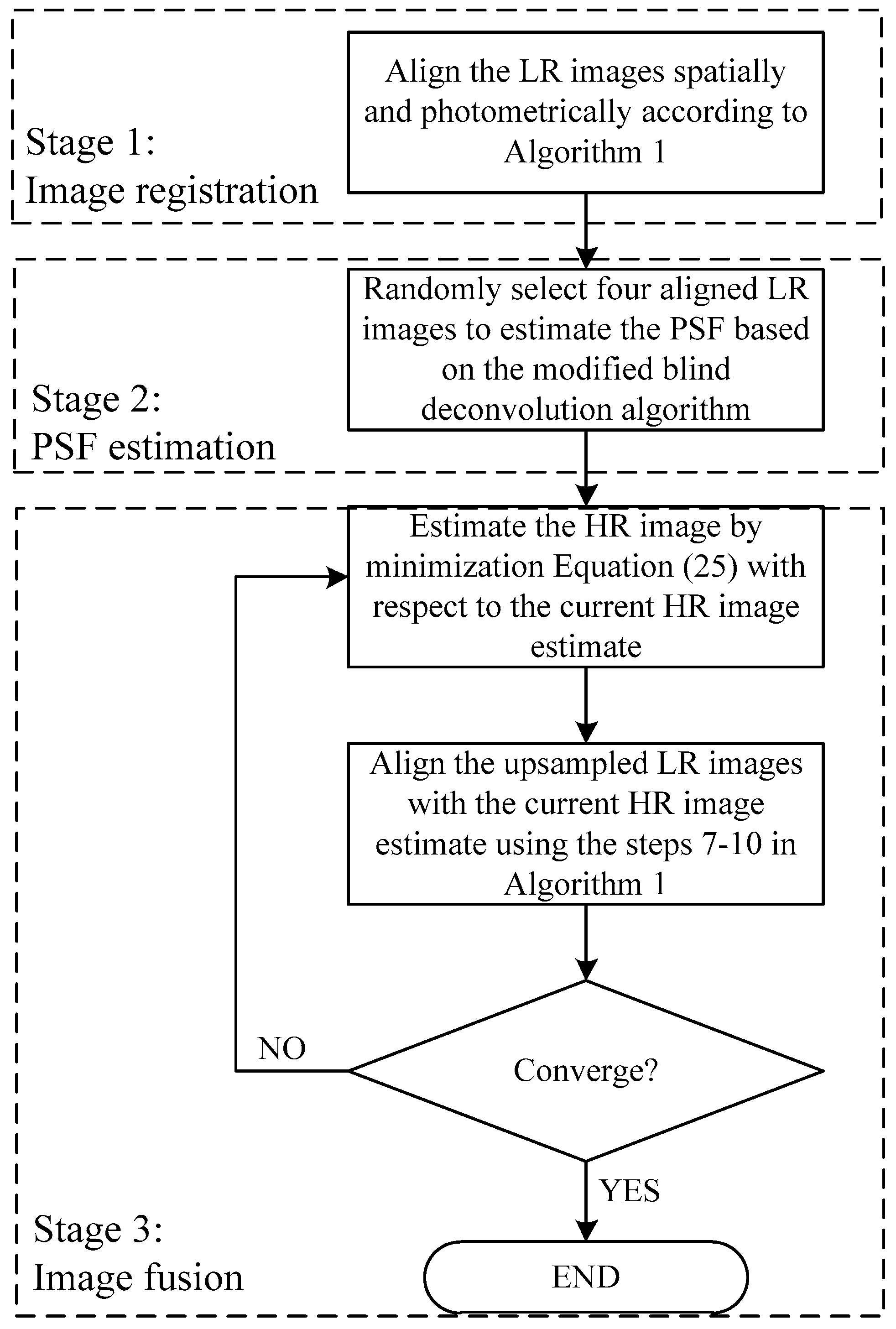
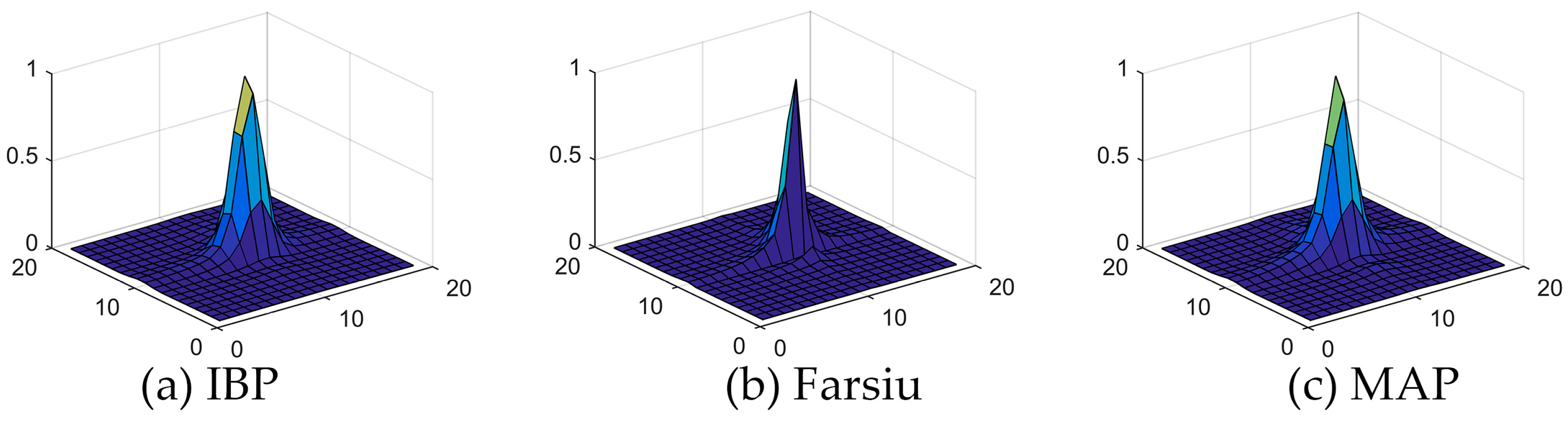
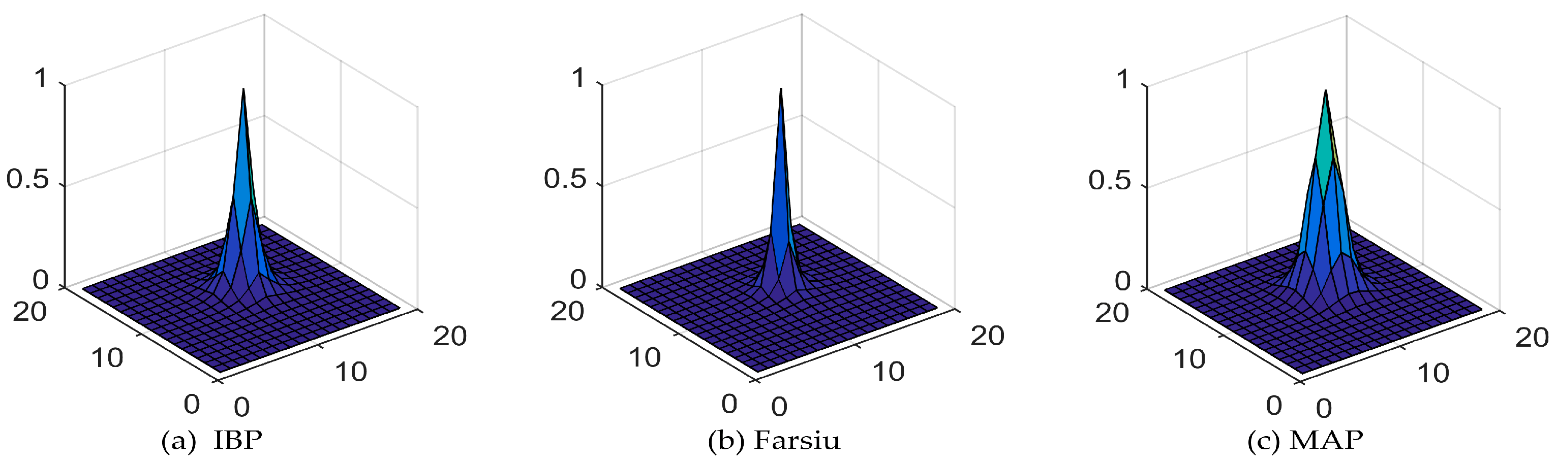
2.3. PSF Estimation
2.4. Image Fusion
3. Results and Discussion
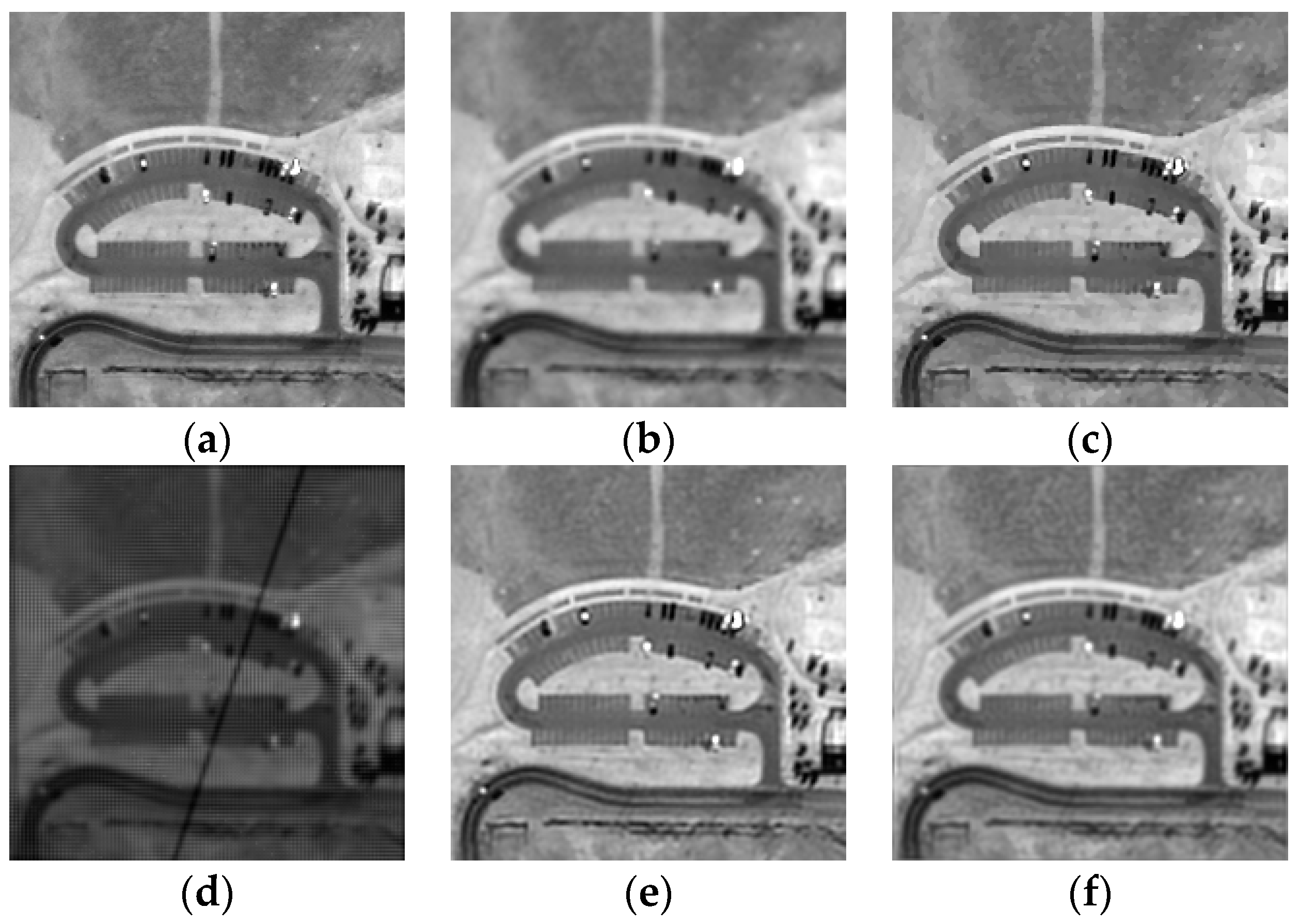
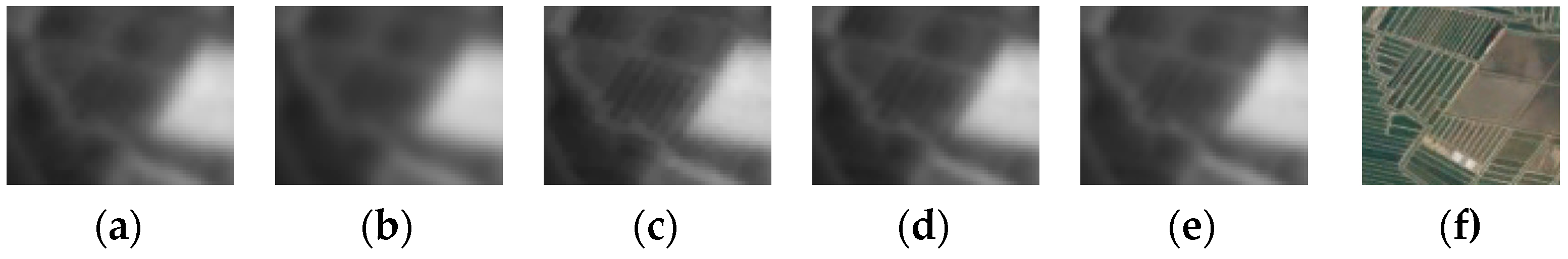
3.1. Simulation Images
- (i)
- Apply random affine transformations generated by their SVD decomposition with translations added, where and are rotation matrices with and uniformly distributed in the range of ; is a diagonal matrix with diagonal elements uniformly distributed in the range of (0.95, 1.05); and the additive horizontal and vertical displacements are uniformly distributed in the range of (–5, 5) pixels.
- (ii)
- Blur the images with a Gaussian point spread function (PSF) with the standard deviation equal to 1.
- (iii)
- Clip images to 0.8 times of the size both horizontally and vertically, so that only overlapped regions are left.
- (iv)
- Downsample the images by a factor of .
- (v)
- Apply photometric parameters with uniformly-distributing contrast gain in the range of (0.9, 1.1) and bias in the range of .
- (vi)
- Make the SNR of the images become 30 dB by adding white Gaussian noise with zero mean.
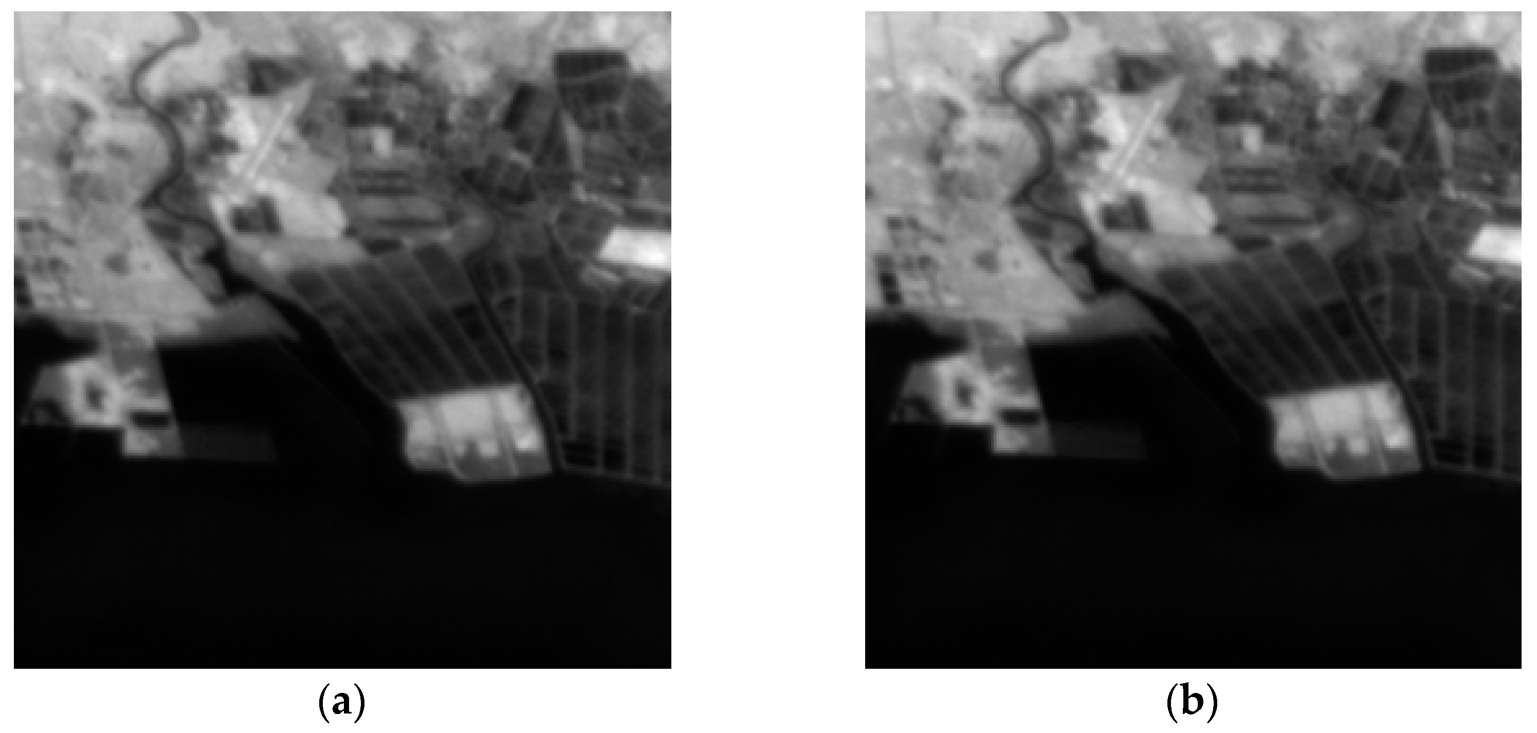
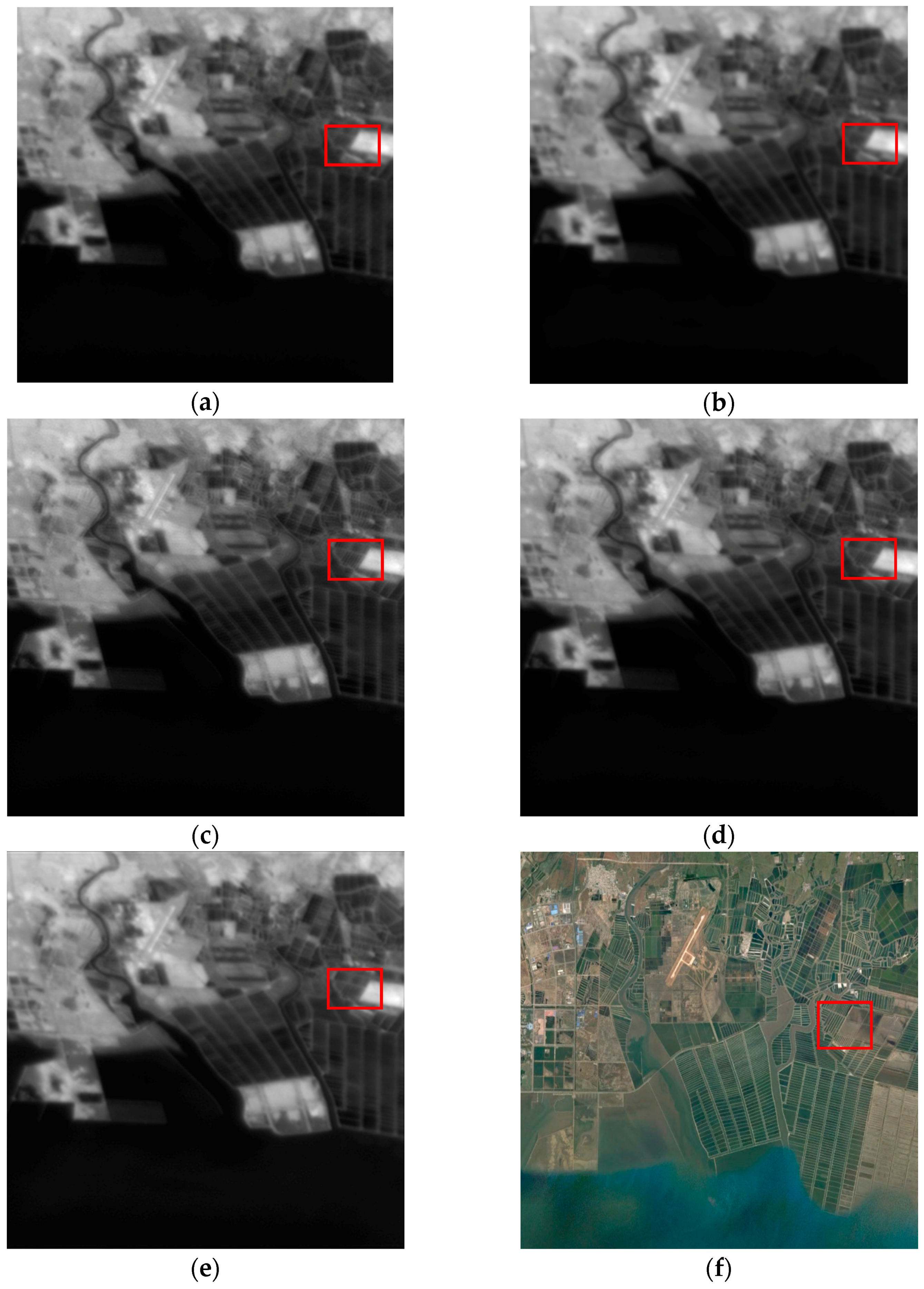
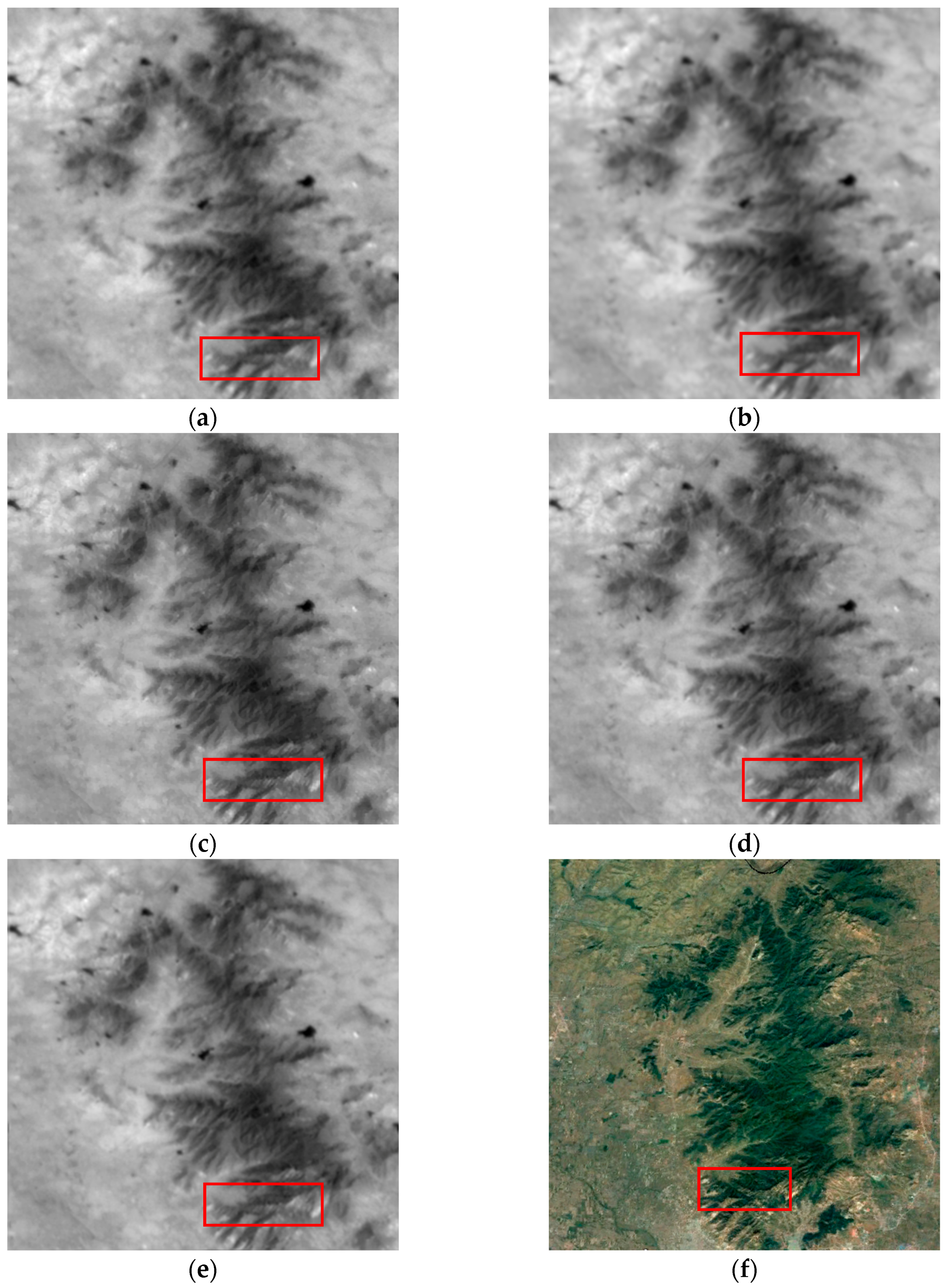
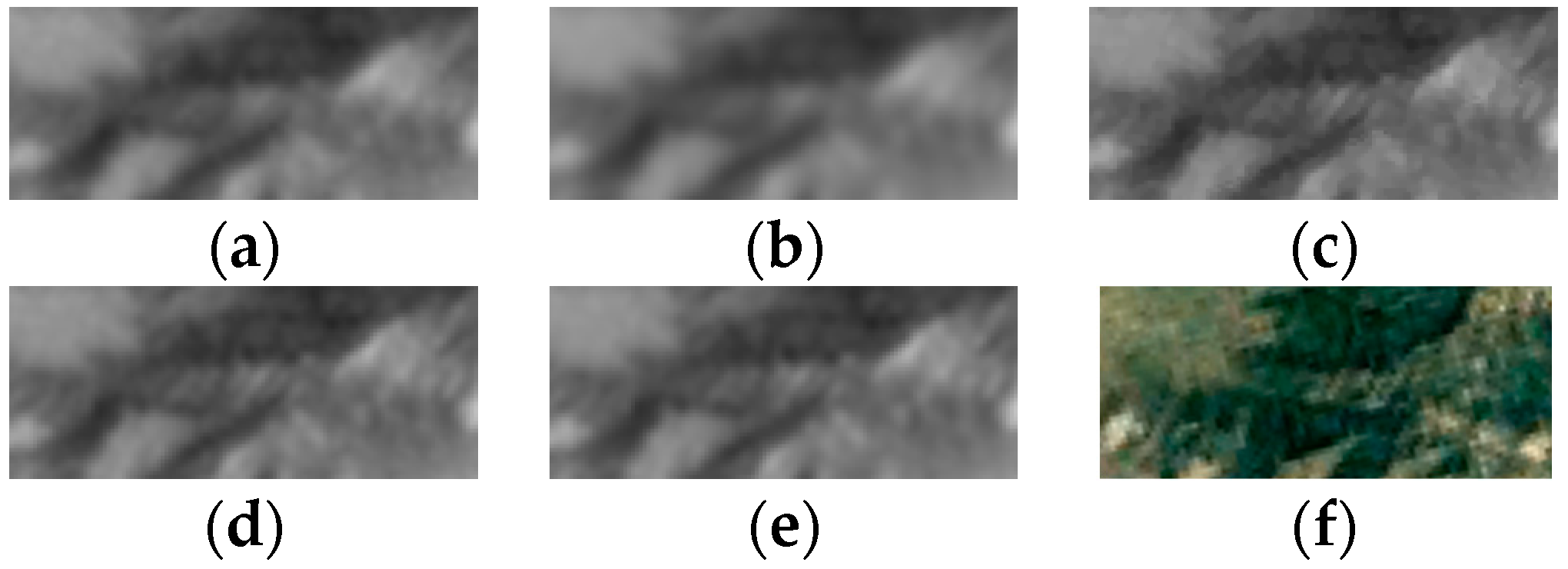
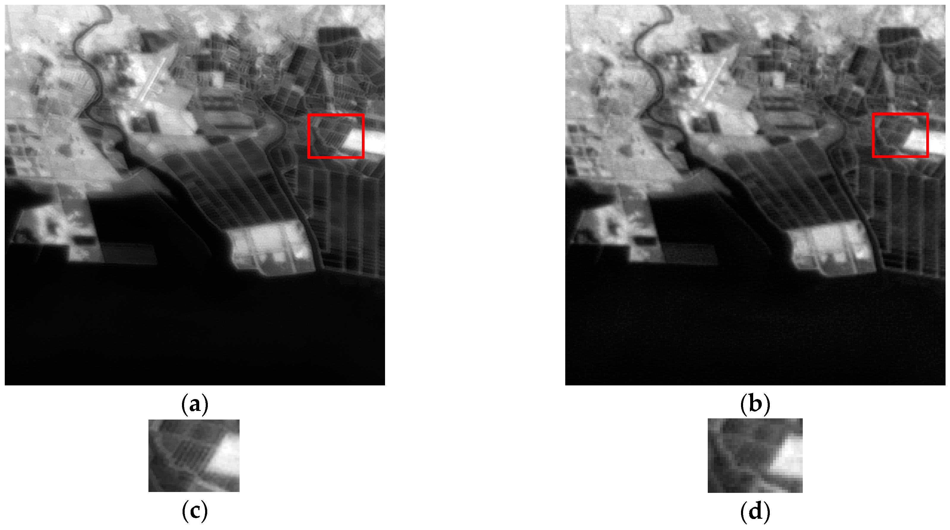
3.2. Real Gaofen-4 Images
3.3. Further Discussion
4. Conclusions
Author Contributions
Conflicts of Interest
References
- Park, S.C.; Park, M.K.; Kang, M.G. Super-resolution image reconstruction: a technical overview. IEEE Signal Process. Mag. 2003, 20, 21–36. [Google Scholar] [CrossRef]
- Alam, M.S.; Bognar, J.G.; Hardie, R.C.; Yasuda, B.J. High resolution infrared image reconstruction using multiple, randomly shifted, low resolution, aliased frames. Proc. SPIE 1997, 3063, 102–112. [Google Scholar]
- Alam, M.S.; Bognar, J.G.; Hardie, R.C.; Yasuda, B.J. Infrared image registration and high-resolution reconstruction using multiple translationally shifted aliased video frames. IEEE Trans. Instrum. Meas. 2000, 49, 915–923. [Google Scholar] [CrossRef]
- Tsai, R.Y. Multiframe image restoration and registration. Adv. Comput. Vis. Image Process. 1984, 1, 317–339. [Google Scholar]
- Yang, J.; Huang, T. Image super-resolution: Historical overview and future challenges. In Super-Resolution Imaging; Milanfar, P., Ed.; CRC Press: Boca Raton, FL, USA, 2010; pp. 1–33. ISBN 978-1-4398-1931-9. [Google Scholar]
- Ur, H.; Gross, D. Improved resolution from subpixel shifted pictures. CVGIP Graph. Models Image Process. 1992, 54, 181–186. [Google Scholar] [CrossRef]
- Stark, H.; Oskoui, P. High-resolution image recovery from image-plane arrays, using convex projections. JOSA A 1989, 6, 1715–1726. [Google Scholar] [CrossRef]
- Patti, A.J.; Sezan, M.I.; Tekalp, A.M. Superresolution video reconstruction with arbitrary sampling lattices and nonzero aperture time. IEEE Trans. Image Process. 1997, 6, 1064–1076. [Google Scholar] [CrossRef] [PubMed]
- Irani, M.; Peleg, S. Improving resolution by image registration. CVGIP Graph. Models Image Process. 1991, 53, 231–239. [Google Scholar] [CrossRef]
- Schultz, R.R.; Stevenson, R.L. Extraction of high-resolution frames from video sequences. IEEE Trans. Image Process. 1996, 5, 996–1011. [Google Scholar] [CrossRef] [PubMed]
- Hardie, R.C.; Barnard, K.J.; Armstrong, E.E. Joint MAP registration and high-resolution image estimation using a sequence of undersampled images. IEEE Trans. Image Process. 1997, 6, 1621–1633. [Google Scholar] [CrossRef] [PubMed]
- Zomet, A.; Rav-Acha, A.; Peleg, S. Robust Super-Resolution. In Proceedings of the IEEE Computer Society Conference on Computer Vision and Pattern Recognition, Kauai, HI, USA, 8–14 December 2001. [Google Scholar]
- Farsiu, S.; Robinson, M.D.; Elad, M.; Milanfar, P. Fast and robust multiframe super resolution. IEEE Trans. Image Process. 2004, 13, 1327–1344. [Google Scholar] [CrossRef] [PubMed]
- Yang, S.; Sun, F.; Wang, M.; Liu, Z.; Jiao, L. Novel Super Resolution Restoration of Remote Sensing Images Based on Compressive Sensing and Example Patches-aided Dictionary Learning. In Proceedings of the International Workshop on Multi-Platform/Multi-Sensor Remote Sensing and Mapping (M2RSM), Xiamen, China, 10–12 January 2011. [Google Scholar]
- Sreeja, S.J.; Wilscy, M. Single Image Super-Resolution Based on Compressive Sensing and TV Minimization Sparse Recovery for Remote Sensing Images. In Proceedings of the IEEE Recent Advances in Intelligent Computational Systems (RAICS), Trivandrum, India, 19–21 December 2013. [Google Scholar]
- Yang, Q.; Wang, H.; Luo, X. Study on the super-resolution reconstruction algorithm for remote sensing image based on compressed sensing. Int. J. Signal Process. Image Process. Pattern Recognit. 2015, 8, 1–8. [Google Scholar] [CrossRef]
- Pan, Z.; Yu, J.; Huang, H.; Hu, S.; Zhang, A.; Ma, H.; Sun, W. Super-resolution based on compressive sensing and structural self-similarity for remote sensing images. IEEE Trans. Geosci. Remote Sens. 2013, 51, 4864–4876. [Google Scholar] [CrossRef]
- Merino, M.T.; Nunez, J. Super-resolution of remotely sensed images with variable-pixel linear reconstruction. IEEE Trans. Geosci. Remote Sens. 2007, 45, 1446–1457. [Google Scholar] [CrossRef]
- Fruchter, A.S.; Hook, R.N. Drizzle: A method for the linear reconstruction of undersampled images. Publ. Astron. Soc. Pac. 2002, 114, 144. [Google Scholar] [CrossRef]
- Shen, H.; Ng, M.K.; Li, P.; Zhang, L. Super-resolution reconstruction algorithm to MODIS remote sensing images. Comput. J. 2007, 52, 90–100. [Google Scholar] [CrossRef]
- Li, F.; Jia, X.; Fraser, D.; Lambert, A. Super resolution for remote sensing images based on a universal hidden Markov tree model. IEEE Trans. Geosci. Remote Sens. 2010, 48, 1270–1278. [Google Scholar]
- Fan, C.; Wu, C.; Li, G.; Ma, J. Projections onto convex sets super-resolution reconstruction based on point spread function estimation of low-resolution remote sensing images. Sensors 2017, 17, 362. [Google Scholar] [CrossRef] [PubMed]
- Jalobeanu, A.; Zerubia, J.; Blanc-Féraud, L. Bayesian estimation of blur and noise in remote sensing imaging. In Blind Image Deconvolution: Theory and Applications; Campisi, P., Egiazarian, K., Eds.; CRC Press: Boca Raton, FL, USA, 2007; pp. 239–275. [Google Scholar]
- Bay, H.; Tuytelaars, T.; Van Gool, L. Surf: Speeded Up Robust Features. In Proceedings of the European Conference on Computer Vision 2006 (ECCV 2006), Graz, Austria, 12–18 October 2006; pp. 404–417. [Google Scholar]
- Thévenaz, P.; Ruttimann, U.E.; Unser, M. A pyramid approach to subpixel registration based on intensity. IEEE Trans. Image Process. 1998, 7, 27–41. [Google Scholar] [CrossRef] [PubMed]
- Fischler, M.A.; Bolles, R.C. Random sample consensus: A paradigm for model fitting with applications to image analysis and automated cartography. Comm. ACM 1981, 24, 381–395. [Google Scholar] [CrossRef]
- Matson, C.L.; Borelli, K.; Jefferies, S.; Beckner, C.C., Jr.; Hege, E.K.; Lloyd-Hart, M. Fast and optimal multiframe blind deconvolution algorithm for high-resolution ground-based imaging of space objects. Appl. Opt. 2009, 48, A75–A92. [Google Scholar] [CrossRef] [PubMed]
- Wang, Z.; Bovik, A.C.; Sheikh, H.R.; Simoncelli, E.P. Image quality assessment: From error visibility to structural similarity. IEEE Trans. Image Process. 2009, 13, 600–612. [Google Scholar] [CrossRef]


| Methods | Bicubic | Our Method | IBP | Farsiu |
|---|---|---|---|---|
| RMSE | 16.44 | 13.36 | 13.94 | 15.90 |
| SSIM | 0.917 | 0.941 | 0.940 | 0.928 |
| Image Number | 2 | 3 | 4 | 5 | 6 | 7 | 8 | 9 | 10 |
|---|---|---|---|---|---|---|---|---|---|
| SNR 1 | 40.5 | 39.7 | 41.0 | 40.3 | 40.6 | 40.1 | 39.7 | 38.5 | 39.1 |
| SNR 2 | 39.9 | 38.1 | 38.0 | 36.4 | 35.5 | 34.4 | 33.4 | 32.2 | 31.7 |
© 2017 by the authors. Licensee MDPI, Basel, Switzerland. This article is an open access article distributed under the terms and conditions of the Creative Commons Attribution (CC BY) license (http://creativecommons.org/licenses/by/4.0/).
Share and Cite
Xu, J.; Liang, Y.; Liu, J.; Huang, Z. Multi-Frame Super-Resolution of Gaofen-4 Remote Sensing Images. Sensors 2017, 17, 2142. https://doi.org/10.3390/s17092142
Xu J, Liang Y, Liu J, Huang Z. Multi-Frame Super-Resolution of Gaofen-4 Remote Sensing Images. Sensors. 2017; 17(9):2142. https://doi.org/10.3390/s17092142
Chicago/Turabian StyleXu, Jieping, Yonghui Liang, Jin Liu, and Zongfu Huang. 2017. "Multi-Frame Super-Resolution of Gaofen-4 Remote Sensing Images" Sensors 17, no. 9: 2142. https://doi.org/10.3390/s17092142
APA StyleXu, J., Liang, Y., Liu, J., & Huang, Z. (2017). Multi-Frame Super-Resolution of Gaofen-4 Remote Sensing Images. Sensors, 17(9), 2142. https://doi.org/10.3390/s17092142