Curve Set Feature-Based Robust and Fast Pose Estimation Algorithm


Abstract
:1. Introduction
2. Curve Set Feature and Rotation Match Feature
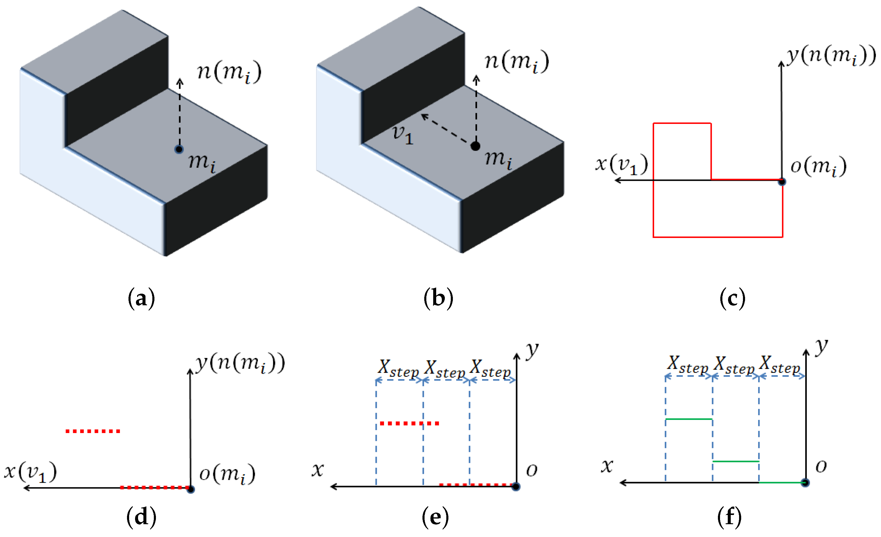
2.1. Curve Set Feature
- Choose a vector starting from and perpendicular to . Build a 2D local coordinate system whose origin is ; the y axis is , and the x axis is .
- All of the points within the local coordinate system whose x value is between zero and are denoted as . Starting from , divide the local coordinate system into small intervals with length (in our experiment, we set as the integer not smaller than the downsampling size) in the x direction. In every small interval, reserve the point with the largest y value, and delete others from to choose visible points.
- Divide the local coordinate system in the x direction again with a larger length . For the points of within the n-th interval, compute the average y value . If there is no point in this interval, set .
- The curve feature of point in the direction of is , . We further define .
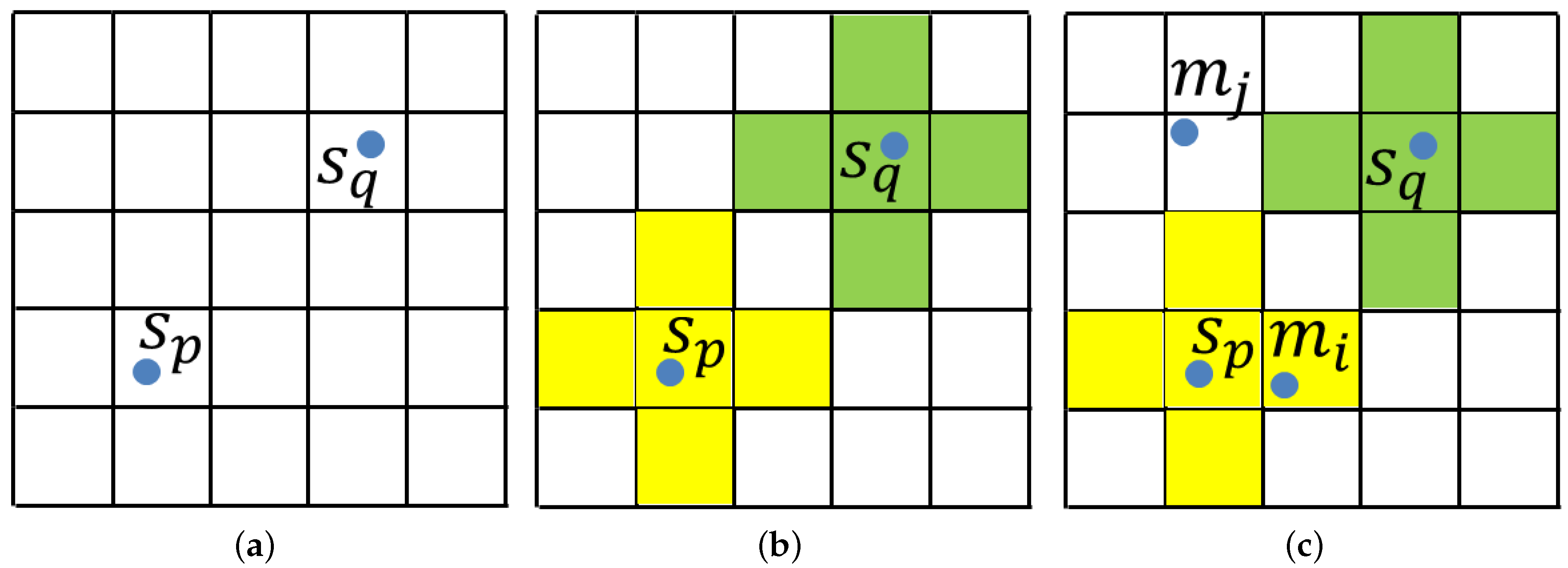
2.2. Compare Curve Set Features
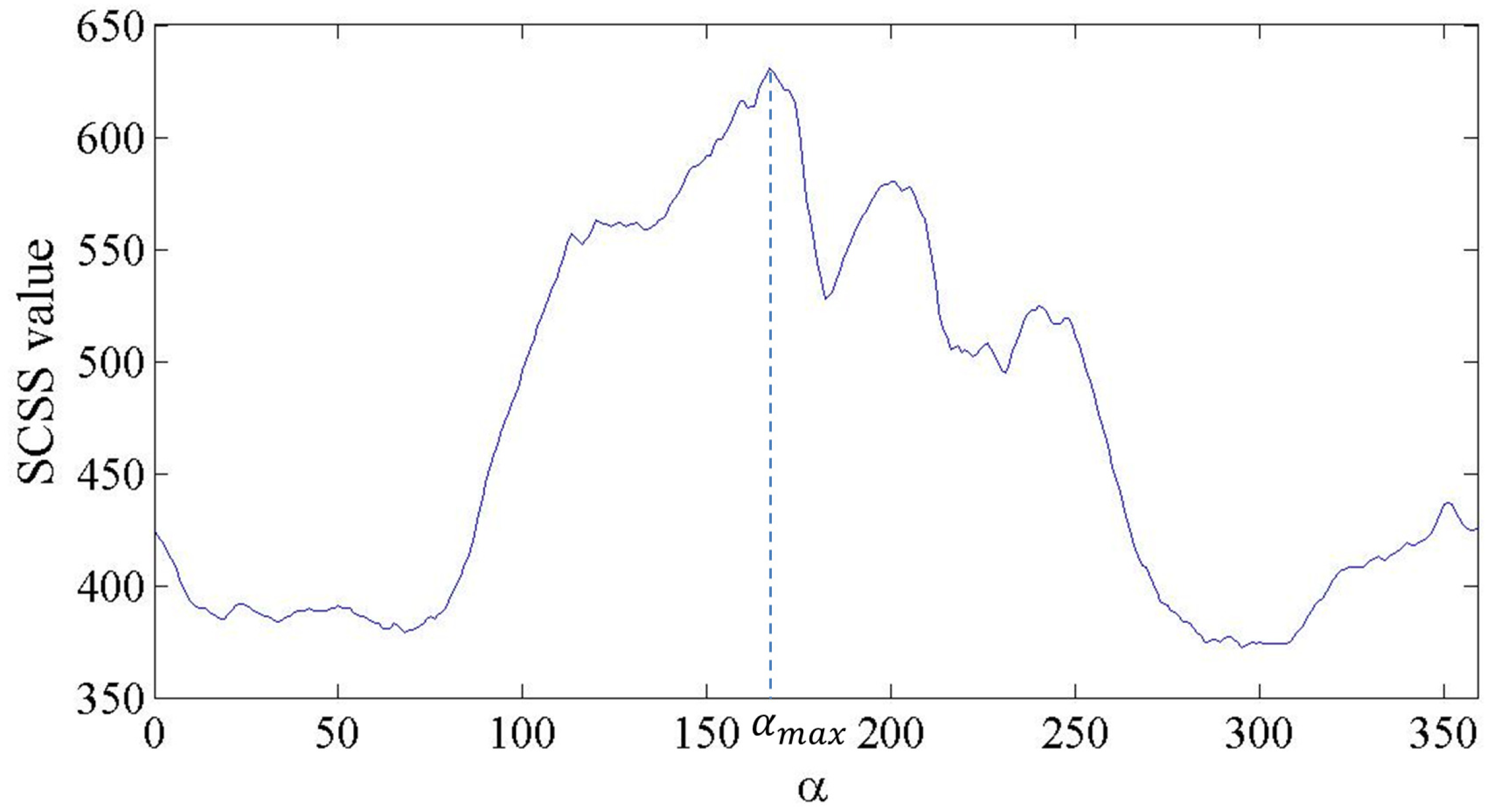
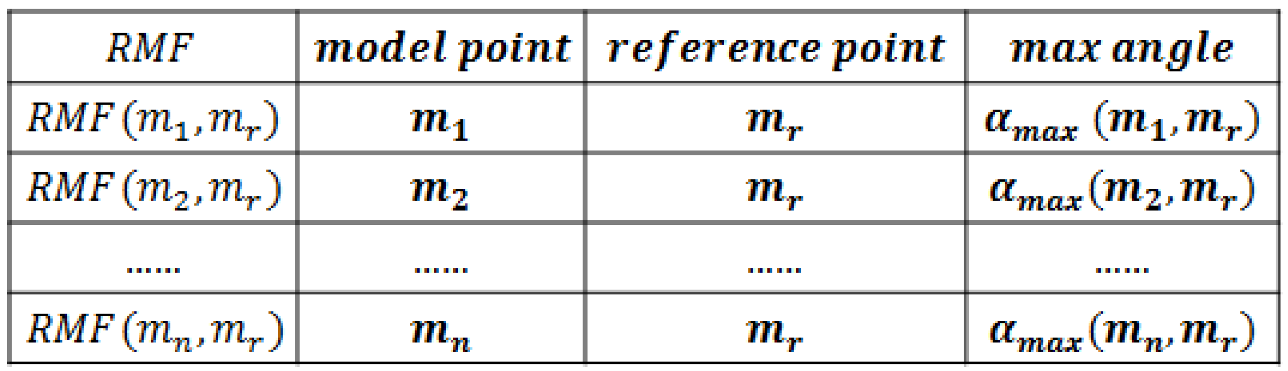
2.3. Rotation Match Feature
- Randomly choose a model point as the reference point.
- From , compute every one degree. Then, save the as when reaches its maximum value.
- The RMF of is the CSS when .
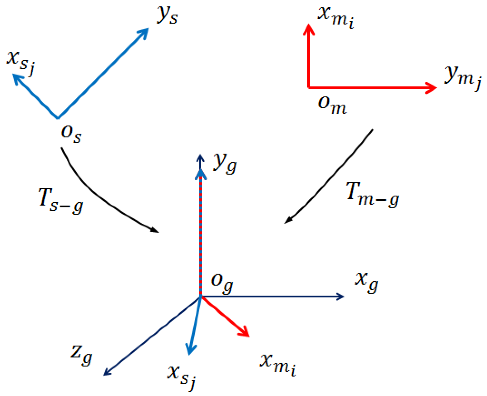
3. Matching Process
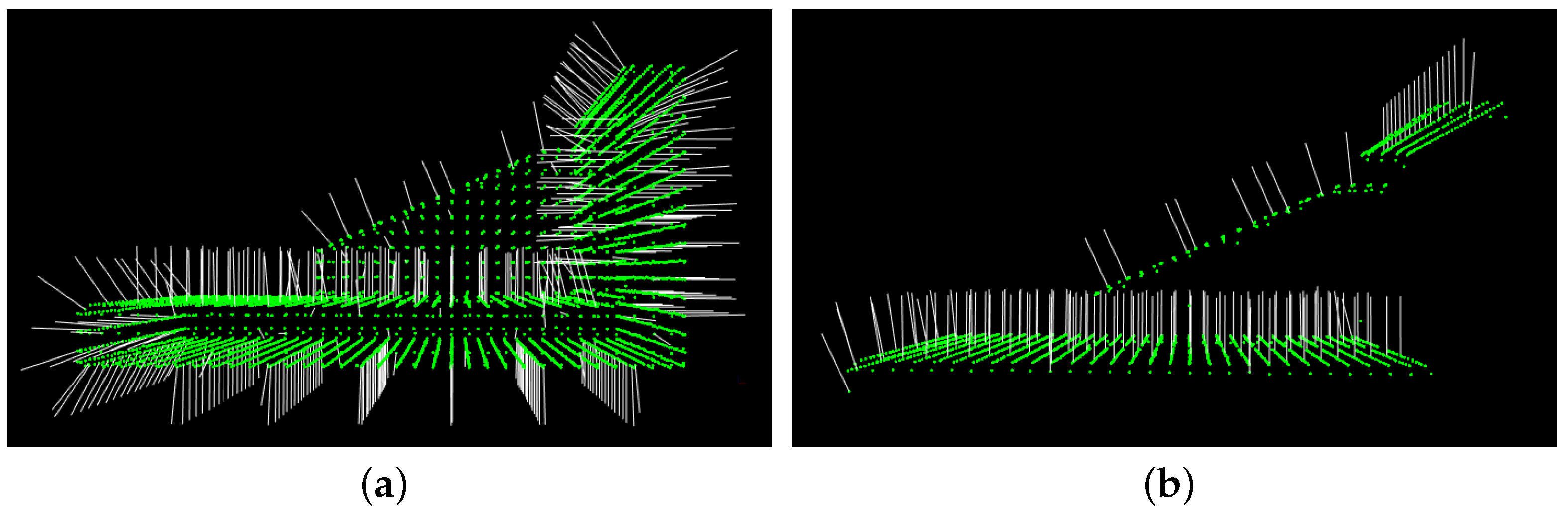
3.1. Normal Estimation and Modification
3.2. Build Model Feature Library
3.3. Scene Cloud Preprocess
3.4. Scene Feature Computation and Nearest Neighbor Search
| Algorithm 1: Compute scene feature and match |
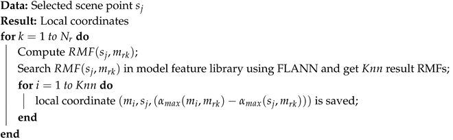 |
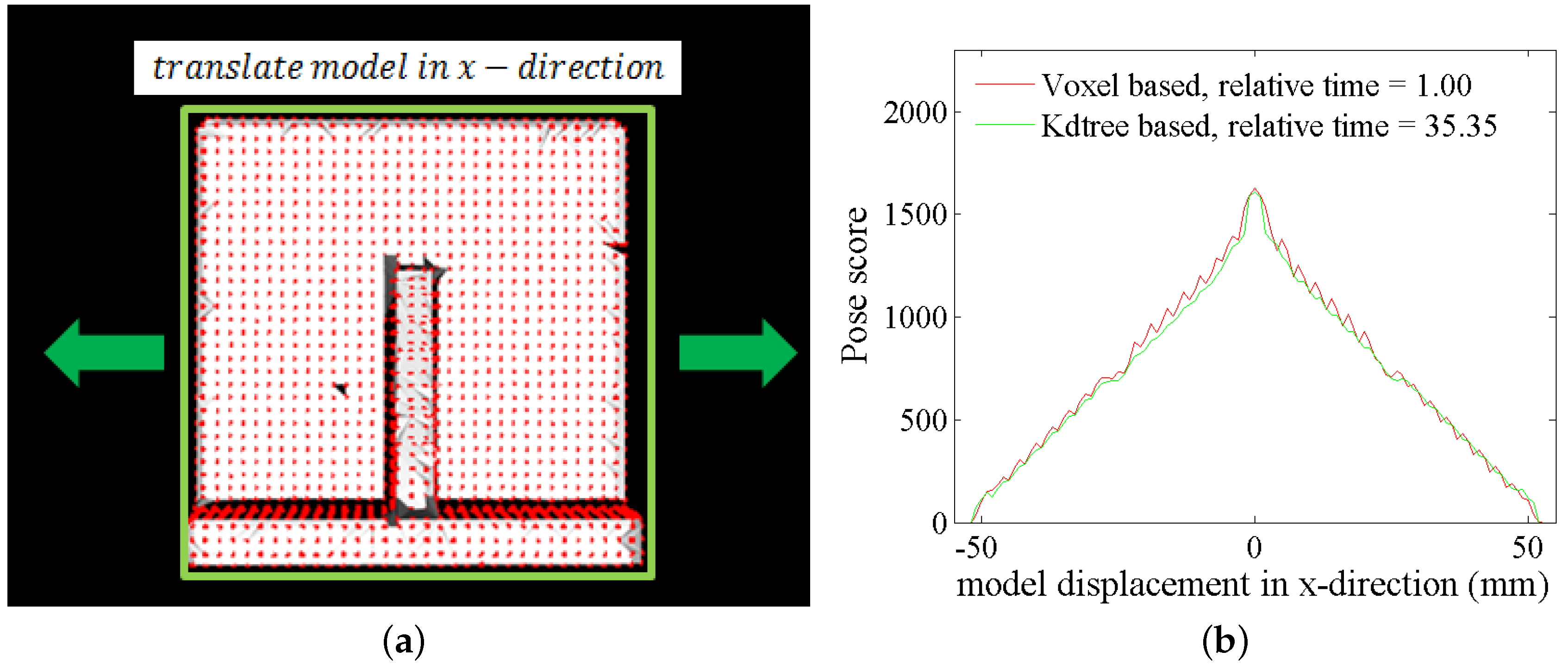
3.5. Pose Verification
| Algorithm 2: Pose verification |
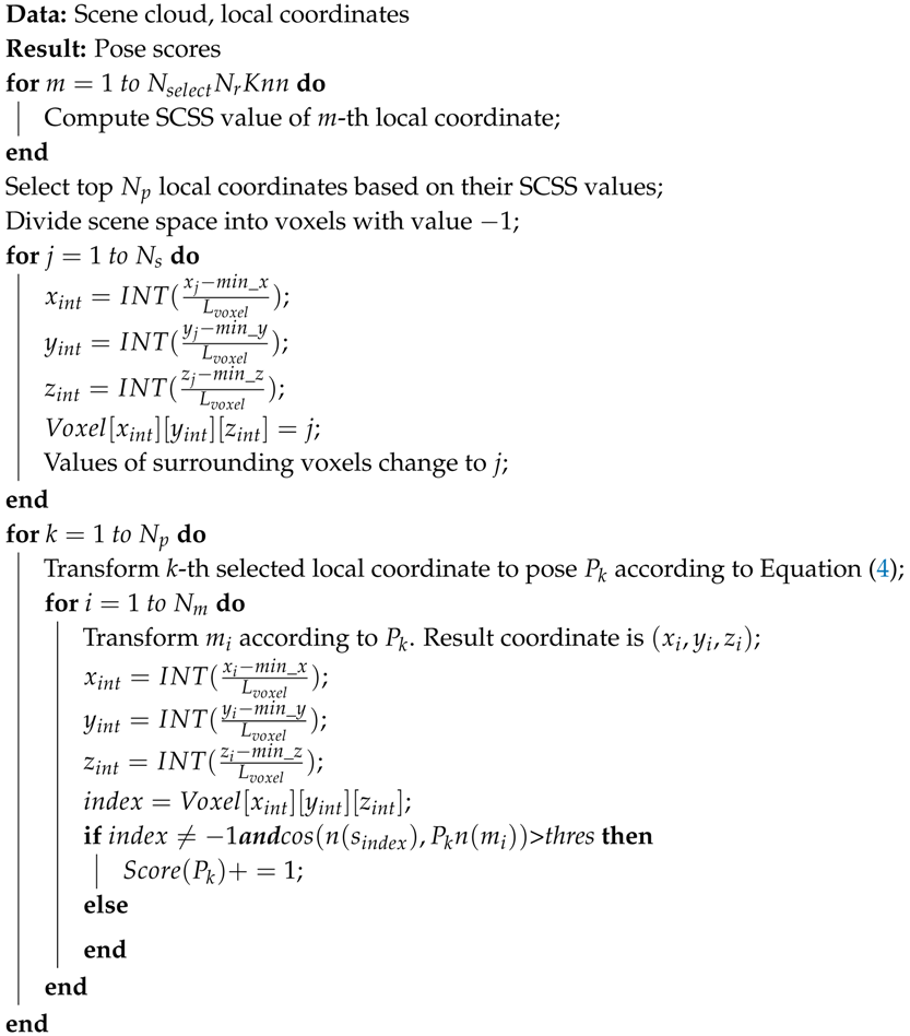 |
3.6. Multiple Pose Detection
- Rank all of the poses with their scores.
- Suppose is the first selected pose. Transform the model cloud into scene space according to .
- For every transformed model point, check whether the value of the voxel it is in is . If not, change the value of all of the voxels sharing the same value with this voxel to .
- Verify the poses with a high grade in Step 1, and choose the pose with the highest grade. is the new pose.
4. Experiment
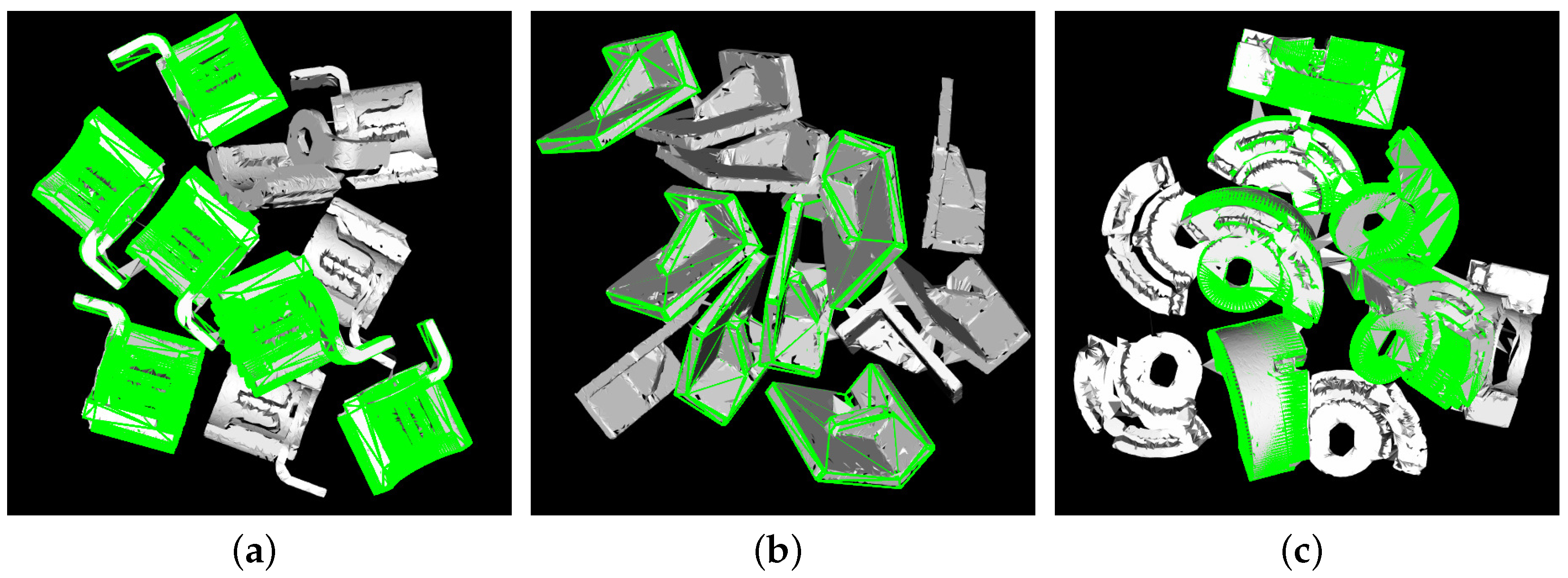
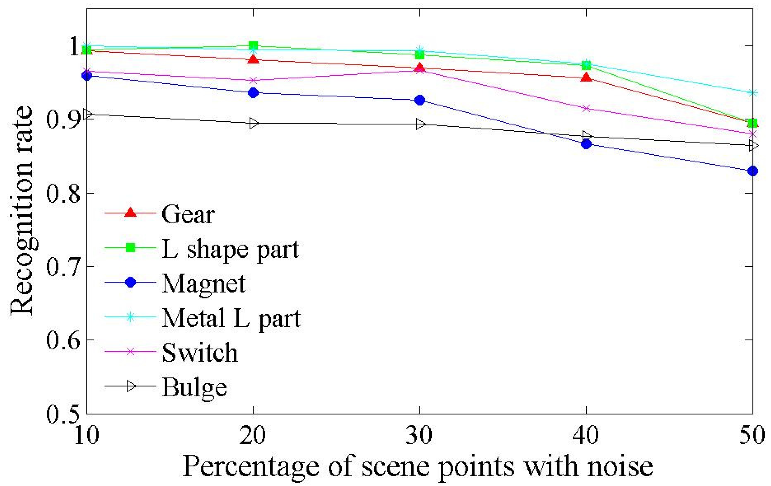
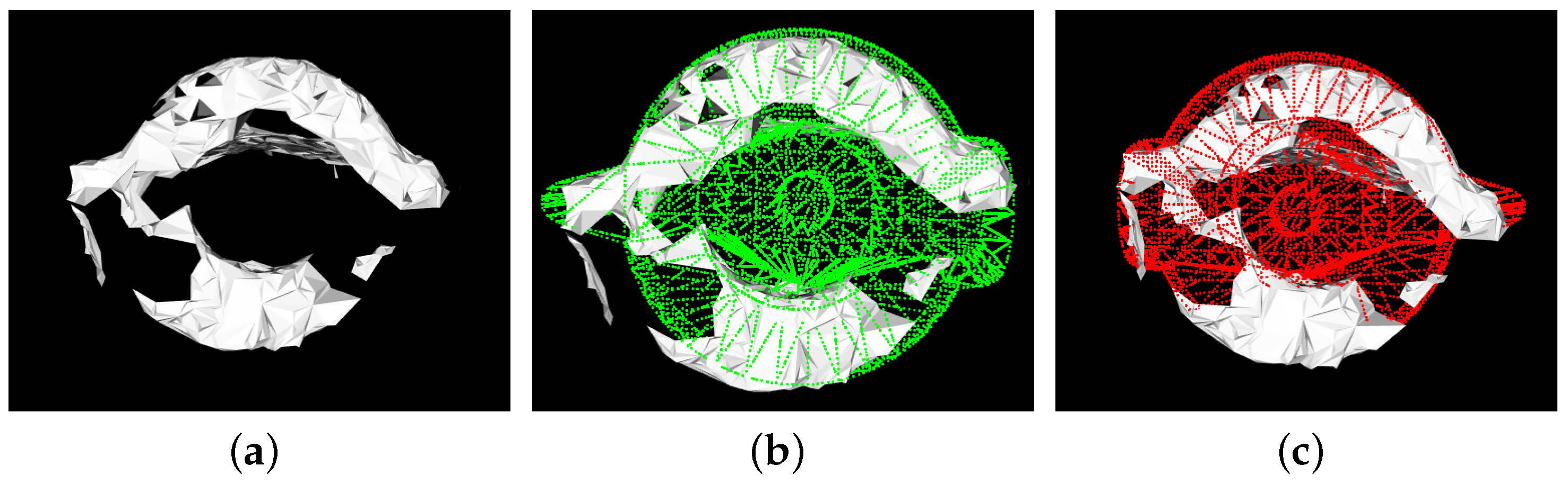
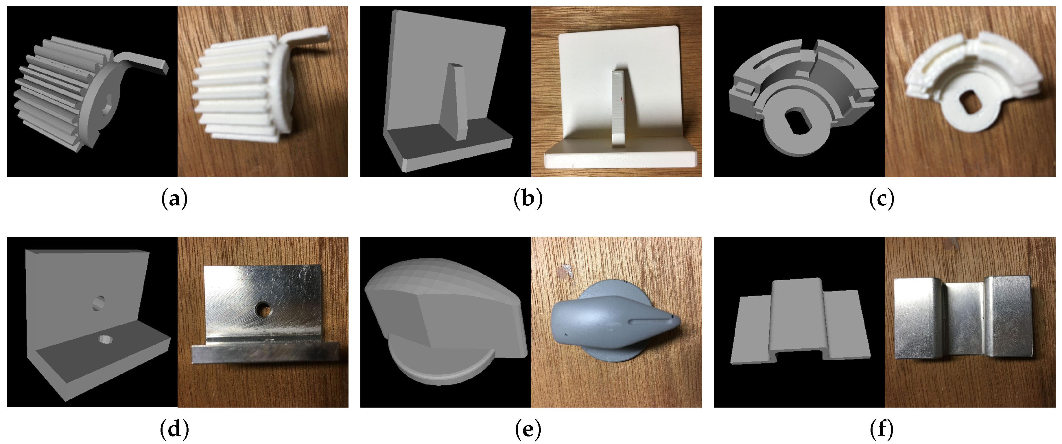
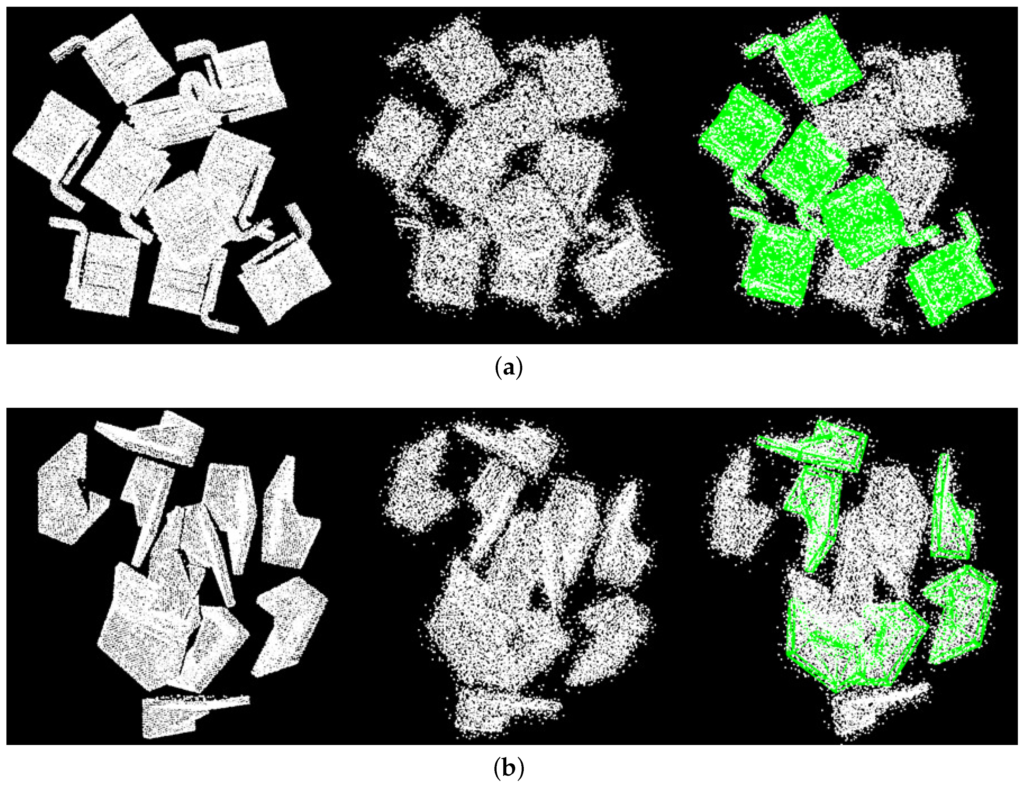
4.1. Synthetic Scenes
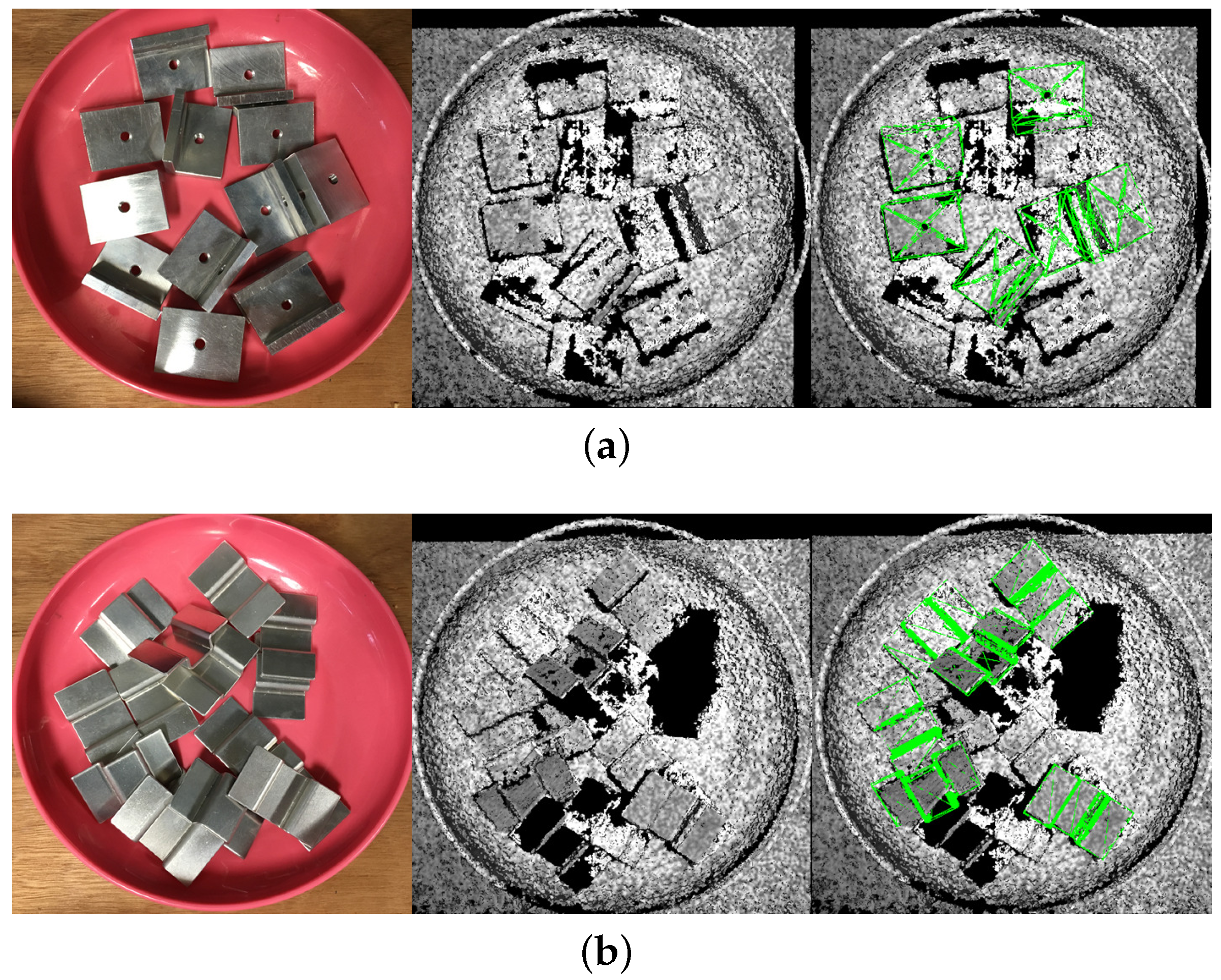
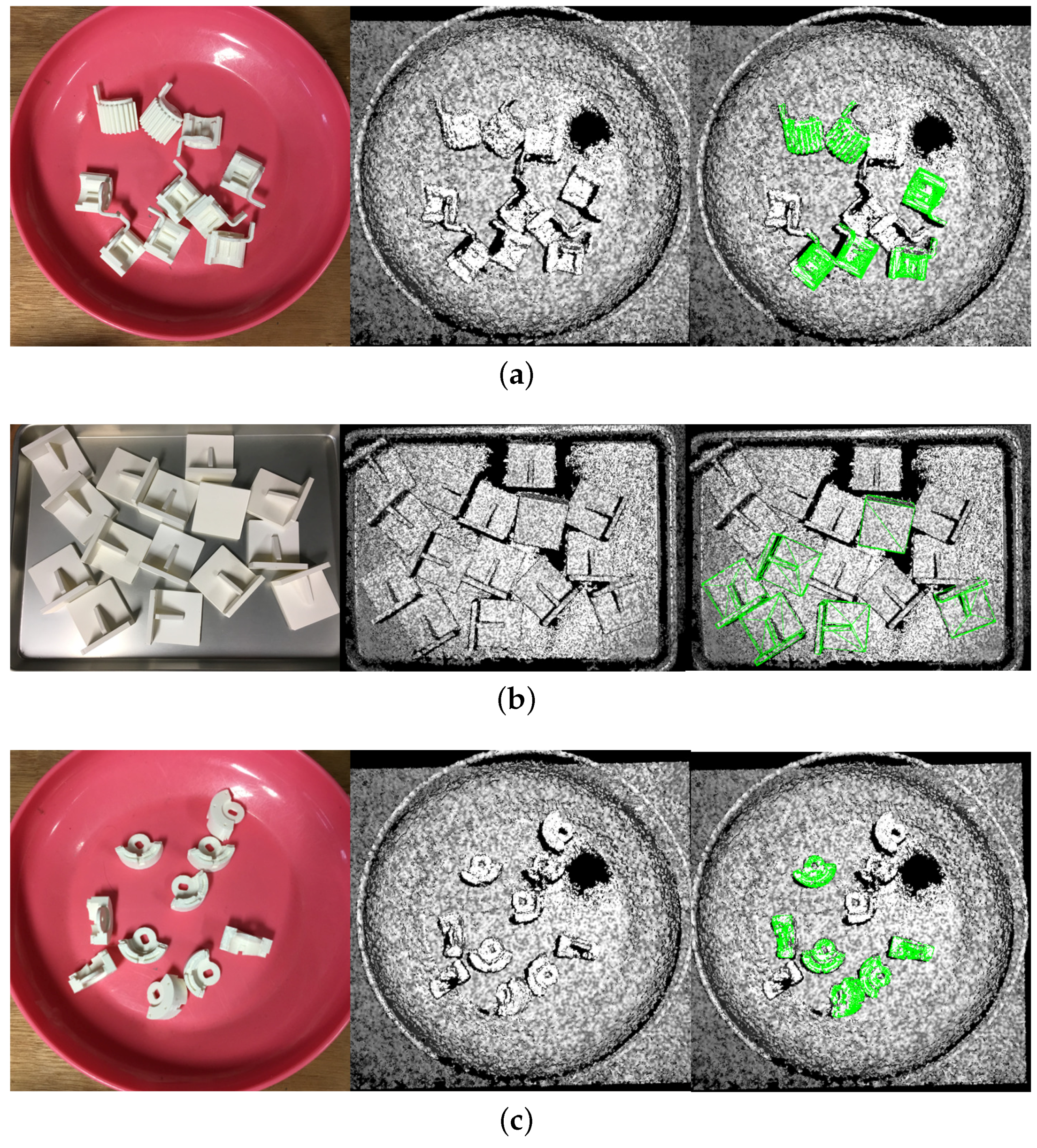
4.2. Real Scenes
5. Conclusions
Acknowledgments
Author Contributions
Conflicts of Interest
References
- Holz, D.; Nieuwenhuisen, M.; Droeschel, D.; Stückler, J.; Berner, A.; Li, J.; Klein, R.; Behnke, S. Active Recognition and Manipulation for Mobile Robot Bin Picking. In The Gearing Up and Accelerating Cross-Fertilization between Academic and Industrial Robotics Research in Europe; Röhrbein, F., Veiga, G., Natale, C., Eds.; Springer: Cham, Switzerland, 2014; pp. 133–153. [Google Scholar]
- Liu, M.Y.; Tuzel, O.; Veeraraghavan, A.; Taguchi, Y.; Marks, T.K.; Chellappa, R. Fast Object Localization and Pose Estimation in Heavy Clutter for Robotic Bin Picking. Int. J. Robot. Res. 2012, 31, 951–973. [Google Scholar] [CrossRef]
- Nieuwenhuisen, M.; Droeschel, D.; Holz, D.; Stückler, J.; Berner, A.; Li, J.; Klein, R.; Behnke, S. Mobile Bin Picking with an Anthropomorphic Service Robot. In Proceedings of the 2013 IEEE International Conference on Robotics and Automation (ICRA), Karlsruhe, Germany, 6–10 May 2013; pp. 2327–2334. [Google Scholar]
- Schnabel, R.; Wessel, R.; Wahl, R.; Klein, R. Shape Recognition in 3D Point-Clouds. In Proceedings of the 16th International Conference in Central Europe on Computer Graphics, Visualization and Computer Vision’ 2008 (WSCG’ 2008), Plzen-Bory, Czech Republic, 4–7 February 2008; pp. 65–72. [Google Scholar]
- Rios-Cabrera, R.; Tuytelaars, T. Discriminatively Trained Templates for 3D Object Detection: A Real Time Scalable Approach. In Proceedings of the 2013 IEEE International Conference on Computer Vision (ICCV), Sydney, Australia, 1–8 December 2013; pp. 2048–2055. [Google Scholar]
- Brachmann, E.; Krull, A.; Michel, F.; Gumhold, S.; Shotton, J.; Rother, C. Learning 6D Object Pose Estimation using 3D Object Coordinates. In Proceedings of the European Conference on Computer Vision (ECCV 2014), Zurich, Switzerland, 6–12 September 2014; pp. 536–551. [Google Scholar]
- Hinterstoisser, S.; Holzer, S.; Cagniart, C.; Ilic, S.; Konolige, K.; Navab, N.; Lepetit, V. Multimodal Templates for Real-Time Detection of Texture-less Objects in Heavily Cluttered Scenes. In Proceedings of the 2011 IEEE International Conference on Computer Vision (ICCV), Barcelona, Spain, 6–13 November 2011; pp. 858–865. [Google Scholar]
- Hinterstoisser, S.; Lepetit, V.; Ilic, S.; Holzer, S.; Bradski, G.; Konolige, K.; Navab, N. Model based training, detection and pose estimation of texture-less 3d objects in heavily cluttered scenes. In Proceedings of the Asian Conference on Computer Vision (ACCV 2012), Daejeon, Korea, 5–9 November 2012; pp. 548–562. [Google Scholar]
- Drost, B.; Ulrich, M.; Navab, N.; Ilic, S. Model globally, match locally: Efficient and robust 3D object recognition. In Proceedings of the 2010 IEEE Conference on Computer Vision and Pattern Recognition (CVPR), San Francisco, CA, USA, 13–18 June 2010; pp. 998–1005. [Google Scholar]
- Choi, C.; Taguchi, Y.; Tuzel, O.; Liu, M.Y. Voting-based pose estimation for robotic assembly using a 3D sensor. In Proceedings of the 2012 IEEE International Conference on Robotics and Automation (ICRA), Saint Paul, MN, USA, 4–18 May 2012; pp. 1724–1731. [Google Scholar]
- Birdal, T.; Ilic, S. Point pair features based object detection and pose estimation revisited. In Proceedings of the 2015 International Conference on 3D Vision (3DV), Lyon, France, 19–22 October 2015; pp. 527–535. [Google Scholar]
- Hinterstoisser, S.; Lepetit, V.; Rajkumar, N.; Konolige, K. Going further with point pair features. In Proceedings of the European Conference on Computer Vision (ECCV 2016), Amsterdam, The Netherlands, 8–16 Octorber 2016; pp. 834–848. [Google Scholar]
- Krull, A.; Brachmann, E.; Michel, F.; Yang, M.Y.; Gumhold, S.; Rother, C. Learning Analysis-by-Synthesis for 6D Pose Estimation in RGB-D Images. In Proceedings of the 2015 IEEE International Conference on Computer Vision (ICCV), Santiago, Chile, 7–13 December 2015; pp. 954–962. [Google Scholar]
- Wu, C.H.; Jiang, S.Y.; Song, K.T. CAD-based pose estimation for random bin-picking of multiple objects using a RGB-D camera. In Proceedings of the 2015 15th International Conference on Control, Automation and Systems (ICCAS), Busan, Korea, 13–16 October 2015; pp. 1645–1649. [Google Scholar]
- Rusu, R.B.; Cousins, S. 3D is here: Point cloud library (PCL). In Proceedings of the International Conference on Robotics and Automation (ICRA), Shanghai, China, 9–13 May 2011; pp. 1–4. [Google Scholar]
- Rusu, R.B.; Bradski, G.; Thibaux, R.; John, H.; Willow, G. Fast 3D recognition and pose using the viewpoint feature histogram. In Proceedings of the 2010 IEEE/RSJ International Conference on Intelligent Robots and Systems (IROS), Taipei, Taiwan, 18–22 October 2010; pp. 2155–2162. [Google Scholar]
- Johnson, A.E.; Hebert, M. Using spin images for efficient object recognition in cluttered 3D scenes. IEEE Trans. Pattern Anal. Mach. Intell. 1999, 21, 433–449. [Google Scholar] [CrossRef]
- Aldoma, A.; Vincze, M.; Blodow, N.; David, G.; Suat, G.; Rusu, R.B.; Bradski, G.; Garage, W. CAD-model recognition and 6DOF pose estimation using 3D cues. In Proceedings of the 2011 IEEE International Conference on Computer Vision Workshops (ICCV Workshops), Barcelona, Spain, 6–13 November 2011; pp. 585–592. [Google Scholar]
- Aldoma, A.; Tombari, F.; Rusu, R.B.; Vincze, M. OUR-CVFH – Oriented, Unique and Repeatable Clustered Viewpoint Feature Histogram for Object Recognition and 6DOF Pose Estimation. Pattern Recognit. 2012, 113–122. [Google Scholar] [CrossRef]
- Muja, M.; Lowe, D.G. Fast approximate nearest neighbors with automatic algorithm configuration. In Proceedings of the International Conference on Computer Vision Theory and Applications (VISAPP’09), Lisboa, Portugal, 5–8 February 2009; pp. 331–340. [Google Scholar]
- Nguyen, D.D.; Ko, J.P.; Jeon, J.W. Determination of 3D object pose in point cloud with cad model. In Proceedings of the 2015 21st Korea-Japan Joint Workshop on Frontiers of Computer Vision (FCV), Mokpo, Korea, 28–30 January 2015; pp. 1–6. [Google Scholar]
- Naoya, C.; Hashimoto, K. Development of Program for Generating Pointcloud of Bin Scene Using Physical Simulation and Perspective Camera Model. In Proceedings of the Robotics and Mechatronics Conference 2017 (ROBOMECH 2017), Fukushima, Japan, 10–12 May 2017. [Google Scholar]


| Models | CSF Default | CSF Fast | CSF No Seg Default | CSF No Seg Fast | OUR-CVFH [19] | PPF [9] |
|---|---|---|---|---|---|---|
| Gear | 97.67% | 91.67% | 96.17% | 82.17% | 97.67% | 43.33% |
| L-shaped part | 100.00% | 99.83% | 98.00% | 56.33% | 94.50% | 79.83% |
| Magnet | 96.00% | 93.17% | 95.50% | 84.17% | 73.33% | 87.83% |
| Metal L part | 99.83% | 88.50% | 99.83% | 88.50% | 82.50% | 97.33% |
| Switch | 95.33% | 91.00% | 97.83% | 90.83% | 65.50% | 96.33% |
| Bulge | 95.33% | 93.33% | 94.67% | 94.17% | 89.33% | 38.83% |
| Average | 97.36% | 92.92% | 97.00% | 82.69% | 83.84% | 73.92% |
| Models | CSF Default | CSF Fast | CSF No Seg Default | CSF No Seg Fast | OUR-CVFH [19] | PPF [9] |
|---|---|---|---|---|---|---|
| Gear | 215 | 78 | 225 | 80 | 1327 | 2579 |
| L-shaped part | 167 | 60 | 199 | 77 | 1078 | 2249 |
| Magnet | 260 | 91 | 233 | 98 | 1012 | 4266 |
| Metal L part | 167 | 70 | 199 | 73 | 553 | 1525 |
| Switch | 245 | 65 | 219 | 107 | 750 | 4297 |
| Bulge | 185 | 62 | 192 | 69 | 445 | 979 |
| Average | 207 | 71 | 211 | 84 | 861 | 2649 |
| Relative time | 2.92 | 1.00 | 2.97 | 1.18 | 12.12 | 37.31 |
| Models | CSF Default | CSF Fast | CSF No Seg Default | CSF No Seg Fast | OUR-CVFH [19] | PPF [9] |
|---|---|---|---|---|---|---|
| Gear | 87.33% | 78.00% | 87.33% | 71.33% | 75.33% | 74.67% |
| L shape part | 96.00% | 84.00% | 94.67% | 75.33% | 27.33% | 60.00% |
| Magnet | 90.67% | 78.00% | 95.33% | 72.67% | 62.67% | 86.67% |
| Average | 91.33% | 80.00% | 92.44% | 73.11% | 55.11% | 73.78% |
© 2017 by the authors. Licensee MDPI, Basel, Switzerland. This article is an open access article distributed under the terms and conditions of the Creative Commons Attribution (CC BY) license (http://creativecommons.org/licenses/by/4.0/).
Share and Cite
Li, M.; Hashimoto, K. Curve Set Feature-Based Robust and Fast Pose Estimation Algorithm. Sensors 2017, 17, 1782. https://doi.org/10.3390/s17081782
Li M, Hashimoto K. Curve Set Feature-Based Robust and Fast Pose Estimation Algorithm. Sensors. 2017; 17(8):1782. https://doi.org/10.3390/s17081782
Chicago/Turabian StyleLi, Mingyu, and Koichi Hashimoto. 2017. "Curve Set Feature-Based Robust and Fast Pose Estimation Algorithm" Sensors 17, no. 8: 1782. https://doi.org/10.3390/s17081782
APA StyleLi, M., & Hashimoto, K. (2017). Curve Set Feature-Based Robust and Fast Pose Estimation Algorithm. Sensors, 17(8), 1782. https://doi.org/10.3390/s17081782