Optimization Techniques for Design Problems in Selected Areas in WSNs: A Tutorial

Abstract
:| Contents | ||
| I | Introduction | 4 |
| II | Overview on Mathematical Optimization | 7 |
| 1 | The History of Optimization | 8 |
| 2 | Introduction to Mathematical Programming | 9 |
| 3 | Linear Programming Problems | 9 |
| 3.1 Solving LPs . . . . . . . . . . . . . . . . . . . . . . . . . . . . . . . . . . . . . . . . . . . . . . . . . . . . . . . . . . . . . . . . . . . . . . . . . . . . . . . . . . . . . . . . . . | 10 | |
| 3.1.1 Simplex Method . . . . . . . . . . . . . . . . . . . . . . . . . . . . . . . . . . . . . . . . . . . . . . . . . . . . . . . . . . . . . . . . . . . . . . . . . . . . . . . . . | 10 | |
| 3.1.2 Karmarkar’s Algorithm . . . . . . . . . . . . . . . . . . . . . . . . . . . . . . . . . . . . . . . . . . . . . . . . . . . . . . . . . . . . . . . . . . . . . . . . . . . | 11 | |
| 3.1.3 On the Efficiency of Simplex and Karmarkar’s Algorithms . . . . . . . . . . . . . . . . . . . . . . . . . . . . . . . . . . . . . . . . . . . . . | 12 | |
| 3.2 Linear Duality . . . . . . . . . . . . . . . . . . . . . . . . . . . . . . . . . . . . . . . . . . . . . . . . . . . . . . . . . . . . . . . . . . . . . . . . . . . . . . . . . . . . . . . . | 12 | |
| 3.2.1 The Dual Simplex . . . . . . . . . . . . . . . . . . . . . . . . . . . . . . . . . . . . . . . . . . . . . . . . . . . . . . . . . . . . . . . . . . . . . . . . . . . . . . . . | 13 | |
| 4 | Network Flow Programming Models | 13 |
| 4.1 Terminology . . . . . . . . . . . . . . . . . . . . . . . . . . . . . . . . . . . . . . . . . . . . . . . . . . . . . . . . . . . . . . . . . . . . . . . . . . . . . . . . . . . . . . . . . | 15 | |
| 4.2 Special Classes of NFPs . . . . . . . . . . . . . . . . . . . . . . . . . . . . . . . . . . . . . . . . . . . . . . . . . . . . . . . . . . . . . . . . . . . . . . . . . . . . . . . . | 16 | |
| 4.2.1 Transportation Problem . . . . . . . . . . . . . . . . . . . . . . . . . . . . . . . . . . . . . . . . . . . . . . . . . . . . . . . . . . . . . . . . . . . . . . . . . . | 16 | |
| 4.2.2 Assignment Problem . . . . . . . . . . . . . . . . . . . . . . . . . . . . . . . . . . . . . . . . . . . . . . . . . . . . . . . . . . . . . . . . . . . . . . . . . . . . . | 17 | |
| 4.2.3 Transshipment Problem . . . . . . . . . . . . . . . . . . . . . . . . . . . . . . . . . . . . . . . . . . . . . . . . . . . . . . . . . . . . . . . . . . . . . . . . . . | 18 | |
| 4.2.4 Shortest Path Problems . . . . . . . . . . . . . . . . . . . . . . . . . . . . . . . . . . . . . . . . . . . . . . . . . . . . . . . . . . . . . . . . . . . . . . . . . . . | 19 | |
| 4.2.5 Maximum Flow Problems . . . . . . . . . . . . . . . . . . . . . . . . . . . . . . . . . . . . . . . . . . . . . . . . . . . . . . . . . . . . . . . . . . . . . . . . . | 20 | |
| 4.2.6 Minimum Spanning Tree (MST) . . . . . . . . . . . . . . . . . . . . . . . . . . . . . . . . . . . . . . . . . . . . . . . . . . . . . . . . . . . . . . . . . . . . | 21 | |
| 4.2.7 Minimum Cost Network Flow Problems . . . . . . . . . . . . . . . . . . . . . . . . . . . . . . . . . . . . . . . . . . . . . . . . . . . . . . . . . . . . . | 21 | |
| 5 | Fundamentals of Nonlinear Optimization | 22 |
| 5.1 Lagrange Functions and Multipliers . . . . . . . . . . . . . . . . . . . . . . . . . . . . . . . . . . . . . . . . . . . . . . . . . . . . . . . . . . . . . . . . . . . . . | 25 | |
| 5.2 Karush-Kuhn-Tucker (KKT) Conditions . . . . . . . . . . . . . . . . . . . . . . . . . . . . . . . . . . . . . . . . . . . . . . . . . . . . . . . . . . . . . . . . . . | 25 | |
| 5.2.1 Geometric Interpretation of KKT Necessary Conditions . . . . . . . . . . . . . . . . . . . . . . . . . . . . . . . . . . . . . . . . . . . . . . . . | 26 | |
| 5.3 Duality for Nonlinear Programs . . . . . . . . . . . . . . . . . . . . . . . . . . . . . . . . . . . . . . . . . . . . . . . . . . . . . . . . . . . . . . . . . . . . . . . . . | 26 | |
| 6 | Decomposition Methods | 27 |
| 6.1 Primal Decomposition . . . . . . . . . . . . . . . . . . . . . . . . . . . . . . . . . . . . . . . . . . . . . . . . . . . . . . . . . . . . . . . . . . . . . . . . . . . . . . . . . | 27 | |
| 6.2 Dual Decomposition . . . . . . . . . . . . . . . . . . . . . . . . . . . . . . . . . . . . . . . . . . . . . . . . . . . . . . . . . . . . . . . . . . . . . . . . . . . . . . . . . . . | 28 | |
| III | Optimization in WSN Design Problems | 29 |
| 7 | Routing for Multi-hop WSNs with a Single Immobile Sink | 32 |
| 7.1 System Model and Design Objectives . . . . . . . . . . . . . . . . . . . . . . . . . . . . . . . . . . . . . . . . . . . . . . . . . . . . . . . . . . . . . . . . . . . . | 32 | |
| 7.2 Initial Optimization Problem Formulation . . . . . . . . . . . . . . . . . . . . . . . . . . . . . . . . . . . . . . . . . . . . . . . . . . . . . . . . . . . . . . . . | 32 | |
| 7.3 Reformulation . . . . . . . . . . . . . . . . . . . . . . . . . . . . . . . . . . . . . . . . . . . . . . . . . . . . . . . . . . . . . . . . . . . . . . . . . . . . . . . . . . . . . . . . | 32 | |
| 7.4 Solution Methods . . . . . . . . . . . . . . . . . . . . . . . . . . . . . . . . . . . . . . . . . . . . . . . . . . . . . . . . . . . . . . . . . . . . . . . . . . . . . . . . . . . . . | 32 | |
| 7.4.1 A partially Distributed Algorithm . . . . . . . . . . . . . . . . . . . . . . . . . . . . . . . . . . . . . . . . . . . . . . . . . . . . . . . . . . . . . . . . . . | 32 | |
| 7.4.2 A fully Distributed Algorithm . . . . . . . . . . . . . . . . . . . . . . . . . . . . . . . . . . . . . . . . . . . . . . . . . . . . . . . . . . . . . . . . . . . . . | 33 | |
| 7.5 Important Results . . . . . . . . . . . . . . . . . . . . . . . . . . . . . . . . . . . . . . . . . . . . . . . . . . . . . . . . . . . . . . . . . . . . . . . . . . . . . . . . . . . . . | 33 | |
| 7.6 Discussions of the Results . . . . . . . . . . . . . . . . . . . . . . . . . . . . . . . . . . . . . . . . . . . . . . . . . . . . . . . . . . . . . . . . . . . . . . . . . . . . . . | 34 | |
| 8 | Routing in a delay-tolerant WSN to a Single Mobile Sink | 34 |
| 8.1 System Model and Design Objectives . . . . . . . . . . . . . . . . . . . . . . . . . . . . . . . . . . . . . . . . . . . . . . . . . . . . . . . . . . . . . . . . . . . . | 34 | |
| 8.2 Initial Optimization Problem Formulation . . . . . . . . . . . . . . . . . . . . . . . . . . . . . . . . . . . . . . . . . . . . . . . . . . . . . . . . . . . . . . . . | 34 | |
| 8.3 Comments on the Problem Formulation . . . . . . . . . . . . . . . . . . . . . . . . . . . . . . . . . . . . . . . . . . . . . . . . . . . . . . . . . . . . . . . . . . | 35 | |
| 8.4 Reformulation for the Optimization Problem Formulation . . . . . . . . . . . . . . . . . . . . . . . . . . . . . . . . . . . . . . . . . . . . . . . . . . | 35 | |
| 8.5 Solution Method . . . . . . . . . . . . . . . . . . . . . . . . . . . . . . . . . . . . . . . . . . . . . . . . . . . . . . . . . . . . . . . . . . . . . . . . . . . . . . . . . . . . . | 35 | |
| 8.6 Important Results . . . . . . . . . . . . . . . . . . . . . . . . . . . . . . . . . . . . . . . . . . . . . . . . . . . . . . . . . . . . . . . . . . . . . . . . . . . . . . . . . . . . | 36 | |
| 9 | Joint Routing, Power and Bandwidth Allocation in FDMA WSNs | 36 |
| 9.1 System Model and Design Objectives . . . . . . . . . . . . . . . . . . . . . . . . . . . . . . . . . . . . . . . . . . . . . . . . . . . . . . . . . . . . . . . . . . . | 36 | |
| 9.2 Optimization Problem Formulation . . . . . . . . . . . . . . . . . . . . . . . . . . . . . . . . . . . . . . . . . . . . . . . . . . . . . . . . . . . . . . . . . . . . . | 36 | |
| 9.3 Reformulation: Distributed Global Consensus Problem . . . . . . . . . . . . . . . . . . . . . . . . . . . . . . . . . . . . . . . . . . . . . . . . . . . . | 37 | |
| 9.4 Solution Method . . . . . . . . . . . . . . . . . . . . . . . . . . . . . . . . . . . . . . . . . . . . . . . . . . . . . . . . . . . . . . . . . . . . . . . . . . . . . . . . . . . . . | 37 | |
| 9.5 A Reference Algorithm . . . . . . . . . . . . . . . . . . . . . . . . . . . . . . . . . . . . . . . . . . . . . . . . . . . . . . . . . . . . . . . . . . . . . . . . . . . . . . . | 38 | |
| 9.6 The Obtained Results . . . . . . . . . . . . . . . . . . . . . . . . . . . . . . . . . . . . . . . . . . . . . . . . . . . . . . . . . . . . . . . . . . . . . . . . . . . . . . . . . | 38 | |
| 10 | Routing and Energy Allocation in Rechargeable WSNs with Multiple Sources and Destinations | 39 |
| 10.1 System Model and Design Objectives and Considerations . . . . . . . . . . . . . . . . . . . . . . . . . . . . . . . . . . . . . . . . . . . . . . . . . | 39 | |
| 10.2 Problem Formulation . . . . . . . . . . . . . . . . . . . . . . . . . . . . . . . . . . . . . . . . . . . . . . . . . . . . . . . . . . . . . . . . . . . . . . . . . . . . . . . . | 39 | |
| 10.3 Comments on the Problem Formulation . . . . . . . . . . . . . . . . . . . . . . . . . . . . . . . . . . . . . . . . . . . . . . . . . . . . . . . . . . . . . . . . | 40 | |
| 10.4 Solution Method . . . . . . . . . . . . . . . . . . . . . . . . . . . . . . . . . . . . . . . . . . . . . . . . . . . . . . . . . . . . . . . . . . . . . . . . . . . . . . . . . . . . | 40 | |
| 10.5 Comments and Observations on the Solution Technique . . . . . . . . . . . . . . . . . . . . . . . . . . . . . . . . . . . . . . . . . . . . . . . . . . | 41 | |
| 10.6 Comments on the Experiments and Results . . . . . . . . . . . . . . . . . . . . . . . . . . . . . . . . . . . . . . . . . . . . . . . . . . . . . . . . . . . . . | 41 | |
| 11 | Routing in Multi-hop Single Immobile Sink for Different Objectives under Distance Uncertainties | 42 |
| 11.1 Problem Statement and Design Objectives . . . . . . . . . . . . . . . . . . . . . . . . . . . . . . . . . . . . . . . . . . . . . . . . . . . . . . . . . . . . . . . | 42 | |
| 11.2 Formulations for the Three Problems . . . . . . . . . . . . . . . . . . . . . . . . . . . . . . . . . . . . . . . . . . . . . . . . . . . . . . . . . . . . . . . . . . . | 42 | |
| 11.3 Accounting for Uncertainties in the Formulation . . . . . . . . . . . . . . . . . . . . . . . . . . . . . . . . . . . . . . . . . . . . . . . . . . . . . . . . . | 43 | |
| 11.4 Important Results . . . . . . . . . . . . . . . . . . . . . . . . . . . . . . . . . . . . . . . . . . . . . . . . . . . . . . . . . . . . . . . . . . . . . . . . . . . . . . . . . . . | 44 | |
| 12 | Joint Routing and Scheduling in WSNs with Multiple Sinks having Different Location Possibilities | 45 |
| 12.1 System Model and Design Objectives . . . . . . . . . . . . . . . . . . . . . . . . . . . . . . . . . . . . . . . . . . . . . . . . . . . . . . . . . . . . . . . . . . | 45 | |
| 12.2 Initial Problem Formulation: Time Based Formulation . . . . . . . . . . . . . . . . . . . . . . . . . . . . . . . . . . . . . . . . . . . . . . . . . . . . | 45 | |
| 12.3 Reformulation: Pattern Based Formulation . . . . . . . . . . . . . . . . . . . . . . . . . . . . . . . . . . . . . . . . . . . . . . . . . . . . . . . . . . . . . . | 46 | |
| 12.4 Solution Method: Column Generation Method . . . . . . . . . . . . . . . . . . . . . . . . . . . . . . . . . . . . . . . . . . . . . . . . . . . . . . . . . . . | 46 | |
| 12.5 Important Results . . . . . . . . . . . . . . . . . . . . . . . . . . . . . . . . . . . . . . . . . . . . . . . . . . . . . . . . . . . . . . . . . . . . . . . . . . . . . . . . . . . | 47 | |
| 13 | Delay-Sensitive Routing in Underwater WSNs | 47 |
| 13.1 System Model and Design Objectives . . . . . . . . . . . . . . . . . . . . . . . . . . . . . . . . . . . . . . . . . . . . . . . . . . . . . . . . . . . . . . . . . . | 47 | |
| 13.2 Initial Problem Formulation . . . . . . . . . . . . . . . . . . . . . . . . . . . . . . . . . . . . . . . . . . . . . . . . . . . . . . . . . . . . . . . . . . . . . . . . . . | 47 | |
| 13.3 Comments on the Initial Problem Formulation . . . . . . . . . . . . . . . . . . . . . . . . . . . . . . . . . . . . . . . . . . . . . . . . . . . . . . . . . . | 48 | |
| 13.4 Reformulation . . . . . . . . . . . . . . . . . . . . . . . . . . . . . . . . . . . . . . . . . . . . . . . . . . . . . . . . . . . . . . . . . . . . . . . . . . . . . . . . . . . . . . | 48 | |
| 13.5 Comments on Reformulation . . . . . . . . . . . . . . . . . . . . . . . . . . . . . . . . . . . . . . . . . . . . . . . . . . . . . . . . . . . . . . . . . . . . . . . . . | 48 | |
| 13.6 The Solution Method in and Our Comments on it . . . . . . . . . . . . . . . . . . . . . . . . . . . . . . . . . . . . . . . . . . . . . . . . . . . . . . . . | 48 | |
| 14 | Using Mobile Radio Frequency (RF) Power Charger to Charge the Batteries of Sensors in a WSN | 49 |
| 14.1 System Model and Design Objectives . . . . . . . . . . . . . . . . . . . . . . . . . . . . . . . . . . . . . . . . . . . . . . . . . . . . . . . . . . . . . . . . . . . | 49 | |
| 14.2 Problem Formulation . . . . . . . . . . . . . . . . . . . . . . . . . . . . . . . . . . . . . . . . . . . . . . . . . . . . . . . . . . . . . . . . . . . . . . . . . . . . . . . . | 49 | |
| 14.3 Solution Method . . . . . . . . . . . . . . . . . . . . . . . . . . . . . . . . . . . . . . . . . . . . . . . . . . . . . . . . . . . . . . . . . . . . . . . . . . . . . . . . . . . . | 50 | |
| 14.4 Observations and Comments on the Problem Formulation, Solution Method and Experiments . . . . . . . . . . . . . . . . . . | 50 | |
| 15 | Assignment of Processing Tasks Across Nodes in a WSN | 50 |
| 15.1 System Model and Design Objectives . . . . . . . . . . . . . . . . . . . . . . . . . . . . . . . . . . . . . . . . . . . . . . . . . . . . . . . . . . . . . . . . . . | 50 | |
| 15.2 Initial Optimization Problem Formulation . . . . . . . . . . . . . . . . . . . . . . . . . . . . . . . . . . . . . . . . . . . . . . . . . . . . . . . . . . . . . . | 51 | |
| 15.3 Solution Method . . . . . . . . . . . . . . . . . . . . . . . . . . . . . . . . . . . . . . . . . . . . . . . . . . . . . . . . . . . . . . . . . . . . . . . . . . . . . . . . . . . | 51 | |
| 15.4 Comments on the Solution Method . . . . . . . . . . . . . . . . . . . . . . . . . . . . . . . . . . . . . . . . . . . . . . . . . . . . . . . . . . . . . . . . . . . . | 51 | |
| 16 | Hierarchical Clustering in a Heterogeneous Network | 51 |
| 16.1 System Model and Design Objectives . . . . . . . . . . . . . . . . . . . . . . . . . . . . . . . . . . . . . . . . . . . . . . . . . . . . . . . . . . . . . . . . . . . | 51 | |
| 16.2 Problem Formulation . . . . . . . . . . . . . . . . . . . . . . . . . . . . . . . . . . . . . . . . . . . . . . . . . . . . . . . . . . . . . . . . . . . . . . . . . . . . . . . . | 52 | |
| 16.3 Solution Method . . . . . . . . . . . . . . . . . . . . . . . . . . . . . . . . . . . . . . . . . . . . . . . . . . . . . . . . . . . . . . . . . . . . . . . . . . . . . . . . . . . . | 52 | |
| 16.4 Comments on the Solution Method . . . . . . . . . . . . . . . . . . . . . . . . . . . . . . . . . . . . . . . . . . . . . . . . . . . . . . . . . . . . . . . . . . . . | 52 | |
| 17 | Energy Efficient Co-Operative Broadcasting at the Symbol Level | 52 |
| 17.1 System Model and Design Objectives . . . . . . . . . . . . . . . . . . . . . . . . . . . . . . . . . . . . . . . . . . . . . . . . . . . . . . . . . . . . . . . . . . | 52 | |
| 17.2 Optimization Problem Formulation . . . . . . . . . . . . . . . . . . . . . . . . . . . . . . . . . . . . . . . . . . . . . . . . . . . . . . . . . . . . . . . . . . . . | 53 | |
| 17.3 Comments on the Optimization Problem Formulation . . . . . . . . . . . . . . . . . . . . . . . . . . . . . . . . . . . . . . . . . . . . . . . . . . . . | 53 | |
| 17.4 Optimal Solution Method and Our Related Comments . . . . . . . . . . . . . . . . . . . . . . . . . . . . . . . . . . . . . . . . . . . . . . . . . . . . | 53 | |
| 17.5 Suboptimal Solution Method: A Heuristic Technique . . . . . . . . . . . . . . . . . . . . . . . . . . . . . . . . . . . . . . . . . . . . . . . . . . . . . | 54 | |
| 17.6 Important Numerical Results . . . . . . . . . . . . . . . . . . . . . . . . . . . . . . . . . . . . . . . . . . . . . . . . . . . . . . . . . . . . . . . . . . . . . . . . . | 54 | |
| 17.7 Comments on the Solution Methods and Their Related Experiments . . . . . . . . . . . . . . . . . . . . . . . . . . . . . . . . . . . . . . . . | 54 | |
| 18 | Dispatching of Mobile Sensor Nodes in a WSN to Sense a Region of Interest | 54 |
| 18.1 System Model and Design Objectives . . . . . . . . . . . . . . . . . . . . . . . . . . . . . . . . . . . . . . . . . . . . . . . . . . . . . . . . . . . . . . . . . . . | 54 | |
| 18.2 Problem Formulation . . . . . . . . . . . . . . . . . . . . . . . . . . . . . . . . . . . . . . . . . . . . . . . . . . . . . . . . . . . . . . . . . . . . . . . . . . . . . . . . | 55 | |
| 18.3 Solution Method: Centralized . . . . . . . . . . . . . . . . . . . . . . . . . . . . . . . . . . . . . . . . . . . . . . . . . . . . . . . . . . . . . . . . . . . . . . . . . | 55 | |
| 18.4 Solution Method: Distributed . . . . . . . . . . . . . . . . . . . . . . . . . . . . . . . . . . . . . . . . . . . . . . . . . . . . . . . . . . . . . . . . . . . . . . . . . | 55 | |
| 18.5 Comments on the Solution Methods . . . . . . . . . . . . . . . . . . . . . . . . . . . . . . . . . . . . . . . . . . . . . . . . . . . . . . . . . . . . . . . . . . . | 56 | |
| 19 | Fusion of Delay Sensitive Noise Perturbed Data Sensed by Different Nodes in a Given Cluster | 56 |
| 19.1 System Model and Design Objectives . . . . . . . . . . . . . . . . . . . . . . . . . . . . . . . . . . . . . . . . . . . . . . . . . . . . . . . . . . . . . . . . . . . | 56 | |
| 19.2 Optimization Problem Formulation . . . . . . . . . . . . . . . . . . . . . . . . . . . . . . . . . . . . . . . . . . . . . . . . . . . . . . . . . . . . . . . . . . . . | 57 | |
| 19.3 Comments on the Formulation . . . . . . . . . . . . . . . . . . . . . . . . . . . . . . . . . . . . . . . . . . . . . . . . . . . . . . . . . . . . . . . . . . . . . . . . | 57 | |
| 19.4 Solution Method: Heuristic scheme . . . . . . . . . . . . . . . . . . . . . . . . . . . . . . . . . . . . . . . . . . . . . . . . . . . . . . . . . . . . . . . . . . . . | 58 | |
| 19.5 Comments on the Solution Methods . . . . . . . . . . . . . . . . . . . . . . . . . . . . . . . . . . . . . . . . . . . . . . . . . . . . . . . . . . . . . . . . . . . | 58 | |
| 20 | Energy Optimization in Wireless Visual Sensor Networks While Maintaining Image Quality | 58 |
| 20.1 System Model . . . . . . . . . . . . . . . . . . . . . . . . . . . . . . . . . . . . . . . . . . . . . . . . . . . . . . . . . . . . . . . . . . . . . . . . . . . . . . . . . . . . . . | 58 | |
| 20.2 Formulation . . . . . . . . . . . . . . . . . . . . . . . . . . . . . . . . . . . . . . . . . . . . . . . . . . . . . . . . . . . . . . . . . . . . . . . . . . . . . . . . . . . . . . . . | 59 | |
| 20.3 Solution . . . . . . . . . . . . . . . . . . . . . . . . . . . . . . . . . . . . . . . . . . . . . . . . . . . . . . . . . . . . . . . . . . . . . . . . . . . . . . . . . . . . . . . . . . . . | 60 | |
| 21 | Conclusions | 60 |
Part I
Introduction
- routing for multi-hop WSNs with a single immobile sink [2],
- routing in a delay-tolerant WSN with a single mobile sink [3],
- joint routing, power and bandwidth allocation in FDMA WSNs [4],
- joint energy allocation and routing in WSNs with rechargeable batteries [5],
- routing in multi-hop single fixed sink with different objectives under distance uncertainties [6],
- joint routing and scheduling in WSNs with multiple sinks with different sink location possibilities [7],
- delay sensitive routing for underwater WSNs [8],
- using mobile radio frequency (RF) power charger to charge the batteries of sensors in a WSN [9],
- assignment of data processing tasks across the nodes in WSN [10],
- hierarchical clustering in a heterogeneous network [11],
- energy efficient co-operative broadcasting at the symbol level [12],
- dispatching of mobile sensor nodes in a WSN to sense a particular region of interest [13],
- fusion of delay sensitive noise perturbed data sensed by different nodes in a given cluster [14],
- Energy Optimization in Wireless Visual Sensor Networks While Maintaining Image Quality [15].
- the system model and design objectives,
- problem formulation,
- any reformulation methods,
- solution methods,
- any important results,
- our comments on some or all of the above.
Part II
Overview on Mathematical Optimization
1. The History of Optimization
- A large progress was made early in improving the techniques of OR. After the war, many of the researchers who had participated on OR teams or who had heard about this work were motivated to continue research in that direction, which lead to advancements in the state of the art. A leading example is the simplex method for solving linear programming problems, developed by George Dantzig in 1947.
- Computer revolution which lead to the development of electronic computers. This is because a large amount of computations is usually required to deal most effectively with the complex problems typically considered by OR. Doing this by hand would be impossible, besides the fact that in most of the practical problems, deriving a closed form expression for the solution is not possible neither.
2. Introduction to Mathematical Programming
- Linear Programming (LP): This is the first category of optimization problems that were considered by early scientists and researchers in the OR field. Basically the decision variables are continuous, the objective function and all the constraints are linear in the decision variables. We would recommend the references [23,24,25] as an introduction with many solved examples for LPs.
- Non-Linear Programming (NLP): In this category, we only have continuous variables but either the objective function or at least one of the constraints are non linear in the decision variables. Good references are the text book by the convex optimization pioneers S. Boyd and V. Vandenberghe [26] and Boyd’s notes for his Convex Optimization I (EE364a) and Convex Optimization II (EE364b) courses in the Stanford University [27,28].
- Mixed Integer Linear Programs (MILP): This is a linear program, where a subset of the decision variables have the restriction that they can only take a set of integer values for each. Again the three textbooks in [23,24,25] would be a good reference for an introduction to this type of optimization problems.
- Mixed Integer Non-Linear Programs (MINLP): This is a non linear program in which a subset of the decision variables must take integer values only. A good reference for this type of problems is the monograph in [29], which is a compilation of key MINLP papers published in a number of strong journals in the field of Operations Research. Another can be a textbook by the global optimization pioneer C.A. Floudas [30].
- The amount of radio power at a particular time slot a sensor is going should transmit (power management), this is usually modelled using continuous variables.
- The time instants and/or durations for each sensor node’s transmission (scheduling). Both continuous and integer variables have been used for that purpose.
- The amount of spectrum bandwidth to be used by each sensor node for transmission. Both continuous and integer variables have been used for that purpose.
- The set of links to be used in a WSN. Binary variables have been used to model whether a link would be used or not.
- Modulation schemes, and channel coding rate each node can use on any of its links. Integer variables are mostly a suitable choice for modeling that aspect.
- The data flow rate in bps per link, usually modelled using continuous variables.
3. Linear Programming Problems
- geometrically forms a polyhedron P of a set of infinitely many feasible solutions in the space of the decision variables i.e., , or
- no solution at all for which we say the LP is infeasible.
3.1. Solving LPs
3.1.1. Simplex Method
3.1.2. Karmarkar’s Algorithm
3.1.3. On the Efficiency of Simplex and Karmarkar’s Algorithms
3.2. Linear Duality
- Weak Duality: For any feasible solution to the primal problem given in Equation (1) and any feasible solution for Equation (4), the (z-value for ) ≥ (w-value for ). If a feasible solution to either the primal or the dual problems is obtained, weak duality enables its use to obtain a bound on the objective function value of the other problem.
- Strong Duality: Is a situation when the bounds are equal to each other i.e., , where and are optimum solutions of the primal and dual respectively.
- If the primal is unbounded the dual is infeasible, and vice versa.
- A basis in a primal problem that is feasible is also optimal if and only if the vector is dual feasible, where:
- (a)
- is a vector of costs in the objective function of the standard form of the primal problem (1) that corresponds to the basic variables in the optimal tableau (last tableau obtained) and,
- (b)
- is an matrix whose jth column is the column for the jth basic variable in the standard form of the primal problem (1).
Hence, when the optimal solution for the primal problem is found by the simplex, we also have found the optimal solution to its dual problem.
3.2.1. The Dual Simplex
- Check the sign of the RHS of each constraint. If all are negative then an optimal solution is at hand. Otherwise, at least one constraint has a negative RHS and we go to step 2.
- The most negative basic variable leaves the basis. Select the variable to enter from the row in which the leaving variable is basic (pivot row) using an absolute ratio test. The variable with the maximum absolute value of the corresponding coefficient in row 0 divided by its coefficient in the pivot row.
- An infeasibility is indicated if there exists a constraint for which the corresponding RHS is negative and the coefficient of each of its variables is negative in the current tableau. If the problem is feasible we go back to step 1.
4. Network Flow Programming Models
4.1. Terminology
- Nodes and Arcs: The network flow model consists of nodes and arcs. In the context of modeling a problem, each node, shown as a circle, represents some aspect of the problem, such as a physical location, an individual worker, or a point in time. In WSNs it is commonly the sensor, or could refer to the sensor node in a number of discrete spacial positions if the sensor is mobile for example [3]. Arcs are directed line segments that generally pass from an origin node to a terminal node, although in the case of external flow, an arc may be incident to only one node. If an arc does not have a direction, it is sometimes referred to as an edge.
- Arc Flow: Flow is associated with the network, entering and leaving at the nodes and passing through the arcs. The flow in arc k is . When flow is conserved at the nodes, the total flow entering a node must equal the total flow leaving the node. The arc flows are the decision variables for the network flow programming model.
- External Flows: The external flow at node i, denoted by , is the flow that must enter node i from sources, or leave node i for destinations outside the network. A positive external flow enters the node, and a negative external flow leaves the node. In the network diagram in Figure 2, the external flow is shown in square brackets adjacent to the node. External flows can model for e.g., the required data rate a sensor node should receive when it is the destination of a particular transmission. Also, they can model the source rate of a wireless sensor node that senses an external phenomena and converts it to electrical signal, then encodes it to a digital bit stream having specific bit rate.
- Upper and Lower Bound on Flow: Flow is limited in an arc by lower and upper bounds. Sometimes the term capacity refers to the upper bound on flow. In wireless sensor networks, the capacity depends on the received signal to noise ratio (SNR) at the node on which the flow arc converges to, given the assumption that the network uses time division multiple access (TDMA), and hence a noise limited system. If radio power control is considered in the problem, the capacity becomes a nonlinear logarithmic function in the power decision variable. This is an example of a possible non-linear network flow and capacity problem in a WSN. The capacity of an arc n is given by , where is the bandwidth for the link represented by arc n, is the channel gain for the link and is the transmitted power on the link, given that . In the case power management is not considered, then the transmission power becomes constant instead of a decision variable, and the entire link capacity becomes constant.
- Cost: The criterion for optimality is cost. Associated with each arc k is the cost per unit of flow . Negative values of correspond to revenues. In WSNs, this can be equivalent to the battery energy expended per flow, where our flow would be in bits per second (bps). Therefore the cost has the units Joules-per-bit. In this case, we are assuming the power to be constant, i.e., we have constant arc capacities. A modulation scheme which decides on the number of bits per second is our decision variable on the flows.
- Gain: The arc gain multiplies the flow at the beginning of the arc to obtain the flow at the end of the arc. When a flow is assigned to an arc, this flow leaves the origin node of the arc. The flow entering the terminal node is . The arc’s lower bound, upper bound, and cost all refer to the flow at the beginning of the arc. Gains less than 1 model losses while gains greater than 1 model growth in flow. In the case of WSNs, the arc gain can represent the reciprocal of the path loss, and the flow could be the radio power transmitted by every sensor in the network for a power management problem.
4.2. Special Classes of NFPs
4.2.1. Transportation Problem
4.2.2. Assignment Problem
4.2.3. Transshipment Problem
- If necessary, put the problem into balanced form by adding either a dummy supply point to meet the excess demand or a dummy demand point to absorb the excess supply. Shipments to or from the dummy node will have zero shipping cost.
- Construct a transportation tableau with rows, one for each supply point and transshipment point, and columns, one for each demand point and transshipment point. Each pure supply point i will have a supply equal to its original value . and each pure demand point j will have a demand equal to its original value . Each transshipment point will have a supply equal to and a demand equal to .
- A large cost M is assigned to shipments that are not permissible. A shipment is allowed from a transshipment point to itself and assigned a unit transportation cost of zero i.e., include in the model and set equal to zero for . The transformed model for the example is shown in Figure 6b.
- Obviously, the transportation simplex can then be used to solve the problem.
4.2.4. Shortest Path Problems
4.2.5. Maximum Flow Problems
4.2.6. Minimum Spanning Tree (MST)
- Initialize a tree with a single vertex, chosen arbitrarily from the graph.
- Grow the tree by one edge: of the edges that connect the tree to vertices not yet in the tree, find the minimum-weight edge, and transfer it to the tree.
- Repeat step 2 until all vertices are in the tree.
4.2.7. Minimum Cost Network Flow Problems
- : represents the number of units of flow sent from node i to node j through arc ().
- : represents the net supply (outflow-inflow) at node i.
- : be cost of transporting 1 unit of flow from node i to node j via arc ().
- : be the lower bound on flow through arc (), if there is not lower bound .
- : be the upper bound on flow through arc (), if there is not lower bound .
5. Fundamentals of Nonlinear Optimization
- Feasible points: a point satisfying all the constraints in Equation (6) is a feasible point and is defined as
- Active, inactive constraints: An inequality constraint is called active at a feasible point if , and is called inactive at a feasible point if . The constraints that are active at a feasible point restrict the feasibility domain while the inactive constraints do not impose any restrictions on the feasibility in the neighborhood of , defined as a ball of radius around , .
- Local minimum: is a local minimum of Equation (6) if there exists a ball of radius around , :
- Global minimum: is a global minimum of Equation (6) if
- Feasible direction vector: Let a feasible point . Then any point in a ball of radius around whaich can be written as is a nonzero vector if and only if . A vector is called a feasible direction vector from , if there exists a ball of radius :The set of feasible directions vectors from is called the cone of feasible directions of F at . An important remark is that if is a local minimum of Equation (6) and is a feasible direction vector from , then for sufficiently small we must have
- An improving feasible vector A feasible direction vector at is called an improving feasible direction vector if:An important remark is that for and , is an improving feasible direction vector at .
- Convex function is a function that satisfies:where , this is illustrated in Figure 10. A concave function is a function that satisfies:Strictly convex or concave functions are ones that strictly satisfy the inequalities (7) and (7) respectively.
- Convex set: A set is convex, if and only if a line segment connecting any two points falls entirely in the set . This is illustrated in Figure 11.
- A convex NLP is a minimization problem that consists of a convex objective function and a convex feasible set of solutions (feasible regions). A concave NLP, is a maximization problem in which the objective function is concave, and the feasible region is a convex set of feasible solutions.
5.1. Lagrange Functions and Multipliers
5.2. Karush-Kuhn-Tucker (KKT) Conditions
5.2.1. Geometric Interpretation of KKT Necessary Conditions
5.3. Duality for Nonlinear Programs
6. Decomposition Methods
6.1. Primal Decomposition

6.2. Dual Decomposition

Part III
Optimization in WSN Design Problems
- the design problem,
- the initial optimization problem formulations,
- the design objective,
- the centralized/distributed possible algorithmic implementation to solve the initial formulations,
- any reformulations performed,
- solution algorithms that were proposed,
- whether the proposed algorithms are distributed or centralized,
- the nature of the solution that could be obtained, whether it is suboptimal or global optimal,
- the convergence speed or computational complexity of the solution algorithms.
7. Routing for Multi-hop WSNs with a Single Immobile Sink
7.1. System Model and Design Objectives
7.2. Initial Optimization Problem Formulation
- Decision variables: Continuous flow variables for all links in the network. Each of these variables has a lower bound of zero and an upper bound of the link’s capacity.
- Objective function: Maximizes the minimum life time of all nodes given as where is the initial battery energy for node i, is the energy spent per bit to transmit data from node i to node j on a direct link, is the set of neighbor nodes that have direct arc connections with i, and is the flow decision variable for link .
- Constraint set: Is a linear equality set of conservation of flow constraints for all the nodes in the network. They simply state that the difference between the outgoing flows from each node and its incoming flows should strictly be equal to the data generated by the node itself.
7.3. Reformulation
7.4. Solution Methods
7.4.1. A partially Distributed Algorithm
7.4.2. A fully Distributed Algorithm
7.5. Important Results
7.6. Discussions of the Results
8. Routing in a delay-tolerant WSN to a Single Mobile Sink
8.1. System Model and Design Objectives
8.2. Initial Optimization Problem Formulation
- Decision variables: are all continuous and are classified as follows,
- The actual decision variable sets are the time the sink stays at each location within each tour, these were denoted by , and the data rate from node i to node j while the sink is at position l, that were given as . These two sets were replaced by the variables , which represent the data flow between two nodes i and j with the sink at position l, through the relation .
- represents the the amount of buffered data at node i just as the sink leaves location l.
- T represents the number of cycles the mobile sink makes.
- Objective function: Maximize the number of cycles the mobile sink makes i.e., . This is a linear objective function in one continuous variable.
- Constraint Sets: The interpretation of the constraint sets is as given below,
- Linear equality constraints that combine the transmission flows and buffered data for all possible sink locations to enforce conservation of flow constraints which guarantee that the total incoming flows for node i plus the buffered data is equal to the outgoing flows.
- Non-negativity constraints on all variables that represent the flows, the buffered data and the number of rounds made by the mobile sink.
- A bi-linear quadratic constraint set that guarantees that all the energy expended due to data transmission on the links for all possible sink positions. It was given by where is the energy spent per unit data on the link when the sink is at position l and is the available energy for node i and is the available battery energy for node i.
8.3. Comments on the Problem Formulation
8.4. Reformulation for the Optimization Problem Formulation
8.5. Solution Method
8.6. Important Results
9. Joint Routing, Power and Bandwidth Allocation in FDMA WSNs
9.1. System Model and Design Objectives
9.2. Optimization Problem Formulation
- Decision variables: All the decision variables are continuous non-negative variables. There are three sets, one set of variables is for the power values on the links , the second is for the flow capacities on the links and the third is for the amounts bandwidth spectrum allocated to the links in the network .
- Objective function: is a linear function in the aggregate link powers i.e., (where is the set of links).
- Constraint sets: There are four functional constraint sets, these are,
- a linear equality constraint set in the flow variables for the conservation of data rate flows. These guarantee that for every node the difference between the out-going flows and the sum of the in-going flows is strictly equal to the rate of data generated by each node .
- a convex non-linear constraint set that guarantees that the flows on each link are upper bounded by the Shannon capacity of the link. These constraints are function in both the powers on the links and the bandwidths allocated to the links and are given as, .
- a linear constraint set in the power variables of the links that guarantees that for each node the aggregate transmission power on all its links does not exceed sensor’s battery power, i.e., .
- A linear constraint set in the bandwidth variables that guarantee that the sum of bandwidths allocated on all the links of every node does not exceed the nodes’ pre-allocated bandwidth W, i.e., .
9.3. Reformulation: Distributed Global Consensus Problem
- , where is the set of all links, incoming and outgoing from node i, represent the consensus constraints.
9.4. Solution Method
9.5. A Reference Algorithm
9.6. The Obtained Results
10. Routing and Energy Allocation in Rechargeable WSNs with Multiple Sources and Destinations
10.1. System Model and Design Objectives and Considerations
- Time slotted system with finite number of slots was considered,
- the battery of each sensor is assumed to have an infinite rechargeable capacity,
- multiple sensing sources and multiple destination nodes are considered,
- utility function that reflects the “satisfaction” of the node is associated with each source node when it transmits at an average data rate that is equal to the aggregate amount of data from that source to a particular destination over all time slots averaged over the duration of the frame. It is defined generally to be concave monotonically increasing in the average data rate of the source node.
10.2. Problem Formulation
- Decision variables: All decision variables are continuous variables. There are three sets of decision variables,
- is the amount of data on the outgoing link for time slot t,
- is the amount of data delivered from source to the destination ,
- represents the amount of energy expended by a node s during slot t.
- Objective function: is the sum of individual node utilities where each of these, , is a function of the amount of data delivered from source node to destination node in all T time slots over possibly multiple hops and multiple paths. Each utility function is assumed to be a continuous non-linear concave function. The time parameter in [5] is discrete.
- Constraint sets: There are three constraint sets, these are:
- non-negative flow constraints on the flow variables .
- conservation of flow constraints that are linear constraints in the decision variables that represent the flow and amount of data delivered from a source node to a destination node, and , i.e., .
- The third ensures that the sum of flows emanating from a node i belongs to the set of the different amounts of data in different time slots under a given replenishment profile vector . For any data vector in , there exists an energy vector that achieves that amount of data for a given modulation and coding scheme. The set was proved to be convex in works earlier to [5].
10.3. Comments on the Problem Formulation
- The authors assume that the generic objective function, given as the sum of the utility functions of all sensor nodes, is concave without stating why is this expected. We believe the characteristics of a generic objective function should cover a wide range of possible objective functions. So, it would be interesting to know how concavity is expected for most of the objective functions in similar system models.
- The relation between the amount of data transmitted by a node on a particular time slot and the expended energy for that is not observable in the formulated problem.
- There were no constraints enforced that take into account the amount of available energy for each node. This may lead to a solution which cannot be satisfied due to lack of energy resources.
- Since there are no non-negativity constraints on the variables that represent the amount of energy expended by the sensor, it is not clear how this formulation guarantees non negative solutions for the energy variables.
- The relation between the allocation of energy and the replenishment is not clear in the formulation.
- The problem is just a generic convex optimization problem so the authors state that standard convex optimization algorithms can be used to solve it. The authors then claim that this is still too complex to solve, even for a known replenishment profile. We believe, however, that a more specific problem (a specific objective and a clear connection between variables) could have more embedded useful structure that if exploited could be solved with lower complexity algorithms.
10.4. Solution Method
10.5. Comments and Observations on the Solution Technique
10.6. Comments on the Experiments and Results
- The comparison between the proposed scheme and the reference scheme was only done for the case where the replenishment process assumes to be general. In the general case the proposed solution technique, DualNet, out performed the reference scheme that assumed independent identically distributed (i.i.d) replenishment process. However no comparison experiments were made to show the performance of both schemes if the replenishment process can be modeled as an i.i.d process. Therefore we have no idea which scheme would be better for such a replenishment profile.
- A time slot duration of one minute was used for the numerical experiments in [5]. We believe that this is impractically too large (in practical TDMA systems time slots are in the order of milliseconds). Moreover, it takes more than five thousand time-slots (i.e., 5000 min) for the lower bound to be the closest to the upper bound as shown in Figure 16. This is too impractical in our opinion.
- Even after the lower bound becomes closest to the upper bound (after a long time), it keeps decreasing monotonically again over ten thousand time slots (i.e., ten thousand minutes) by around before starting to increase again.
11. Routing in Multi-hop Single Immobile Sink for Different Objectives under Distance Uncertainties
- minimizing the energy consumed,
- maximizing the data extracted,
- maximizing the network lifetime.
11.1. Problem Statement and Design Objectives
- one for the normalized received energy which is equivalent to the number of received bytes, i.e.,
- and one for the the normalized transmitted energy, which is equivalent to the number of transmitted bytes times a linear function in the transmission distance, i.e.,
- A is the set of nodes in the network,
- is the number of transmitted bytes from node j to node i.
- is the distance from node i to node j and is a constant depending on transceiver parameters.
11.2. Formulations for the Three Problems
- The Minimum Energy Problem:
- Decision variables: are the continuous variables which are the number of bytes transmitted on a link from node i to node j.
- Objective function: is a continuous linear objective function in which is the sum of the transmission and reception normalized energies of all nodes in the network. The objective is to minimize that aggregate energy function.
- Constraints: the first constraint is a minimum data transmission requirement constraint that requires the aggregate data transmitted from all nodes to the sink node, to be greater than a minimum number of bytes. The second and third constraint sets are conservation of flow constraints that require the difference between the amount of data bytes transmitted and received by a node to be less than the available data bytes at the node and greater than zero. The variables have non-zero constraints also.
- The Maximum Data Extraction Problem:
- Decision variables: are which are the number of bytes transmitted on a link from node i to node j.
- Objective function: maximizes the data transmitted to the sink node. It was given as the sum of data bytes transmitted from each node i to the sink node on the arcs . It is a continuous linear objective function.
- Constraints: Besides the conservation of flow and non-negativity constraints in Minimum Energy Problem, there is a set of energy limitation constraints for each node, that guarantees that the the sum of transmitted and received energy for each node does not exceed the available energy of the node, i.e.,Note that in [6], the energy is normalized such that is the number of bytes that could be transmitted with the available energy and the left hand side of the constraint is the amount of bytes transmitted for an expended amount of energy. All constraints are linear and hence the problem is a linear program ignoring the uncertainties.
- Maximum Lifetime Problem:
- Decision variables: are which are the number of bytes transmitted on a link from node i to node j and T which is the variable represents the lifetime of the network.
- Objective function: maximize the lifetime T of the network which is defined as the lifetime of the first sensor whose battery gets depleted, i.e., .
- Constraints: Conservation of flow and non-negativity constraints typical to those in Minimum Energy Problem, in addition a quadratic constraint with bilinear terms that guarantees that the energy expended by transmission of a node i does not exceed its available energy, this is given by:where the left hand side This gives a quadratically constrained program, which is transformed to a linear program by substituting the variable T in the problem with and minimizing the objective function instead of maximizing it.
11.3. Accounting for Uncertainties in the Formulation
- Polyhedral uncertainty sets: Using LP duality, it was shown that optimization problem remains as a linear program with additional variables and constraints.
- Ellipsoidal sets: Using a known closed form solution for an embedded ellipsoidal optimization subproblem with respect to the uncertainty variables, the robust optimization problem becomes a conic convex problem that can be solved by interior point methods in polynomial time. With a simple reformulation trick of replacing the conic component in the objective function with an upper bound linear component and bringing in the conic component in the constraint set, the problem can be rewritten as a second order cone program (SOCP).
11.4. Important Results
12. Joint Routing and Scheduling in WSNs with Multiple Sinks having Different Location Possibilities
12.1. System Model and Design Objectives
12.2. Initial Problem Formulation: Time Based Formulation
- Decision variables: T is a continuous variable that represents the network’s lifetime, is a continuous variable that represents the data rate on the link from node i to node j at a given time t, is a continuous variable that represents the data rate from node i to one of the possible sinks’ positions o at a given time t, is a binary variable that is set only when sink s resides in position o.
- Objective function: is to maximize the lifetime of the network which is given as ,
- Constraint Sets: The constraints sets of the initial formulation are explained below:
- Constraint set 1: is a linear constraint set in the binary variables that guarantees that a possible position o at t can get occupied by no more than one sink node, this is given as , where and are the sets of sink nodes and possible sink positions respectively.
- Constraint set 2: is a linear constraint set in the binary variables that guarantees that sink s at time t can only reside in one location, this is given as .
- Constraint set 3: linear conservation of flow equality constraints in the flow variables and .
- Constraint set 4: variable upper bounds on the flow variables from node to node links that represent the link capacity.
- Constraint set 5: a mixed integer linear constraint in the variables and that impose link capacity on the flows from node i to the possible sink location o if any sink is assigned to that location, otherwise the flow is enforced to be zero. The constraint is where is the capacity of the link .
- Constraint set 6: An energy constraint for each sensor which is an integration of linear terms with respect to the time parameter t with the decision variable T in the upper limit of the integral.
- Constraint set 7: non-negativity constraints on all the decision variables.
12.3. Reformulation: Pattern Based Formulation
- Decision variables:
- the continuous variables which represent the assigned time durations for the possible patterns p,
- continuous variables for the energy consumption rate for node i in pattern p for all nodes and patterns,
- binary decision variables tell whether sink node s is assigned to location o in the pattern placement p for all nodes, sinks and patterns,
- continuous variables for the data rate flow from node i to the sink position o in pattern p for all nodes, sinks and patterns,
- continuous variables for the data flow rate on the link between the nodes i and j in pattern p for all nodes and patterns.
- Objective function: Maximizes the aggregate durations assigned to the patterns which in [7], was stated to be equivalent to the lifetime of the network, i.e., .
- Constraint sets: The same constraint sets for the time-based formulation should be satisfied for each pattern, the energy constraints however are replaced by two constraint sets for each pattern, one is linear and the other is bilinear quadratic. The linear one is an equality constraint that links the energy expended by the node in a given placement pattern with the flow variables and . The bilinear constraint set guarantees that all the energies expended by every node in all pattern durations do not exceed their initial battery energies.
12.4. Solution Method: Column Generation Method
12.5. Important Results
13. Delay-Sensitive Routing in Underwater WSNs
13.1. System Model and Design Objectives
13.2. Initial Problem Formulation
- Decision variables:
- the number of bits transmitted on each link (),
- the transmission time allocated for each link ().
- Objective function: is the sum of all energy consumed on all links in the network. It contains which is a non-deterministic general term that is function in the number of bits to be transmitted on each link and the allocated transmit time . This term represents power consumption which is dependent on the modulation/channel coding schemes used for transmission.
- Constraint sets:
- A linear delay constraint, that takes into account the propagation delay of each link and the transmission delay that is inherent in the allocated transmission time. The total delays on all links from the source sensor nodes to the sink should not exceed a maximum allowable delay T, that was given by where is the propagation delay of link and is the set of next hop candidates that are closer to the sink than i.
- A linear conservation of flow set of constraints for every node that guarantees that difference between incoming and outgoing data is equal to the amount of data generated by the sensor node, that is where is the data generation rate of node i and is the set of neighboring nodes for which i is a next hop candidate.
13.3. Comments on the Initial Problem Formulation
13.4. Reformulation
- is a new variable that represents the energy expended for transmission of data on link .
- is a constant that represents the relation between the logarithm of the power on a particular link with respect to the logarithm of the transmission rate on that link.
13.5. Comments on Reformulation
- Advantages: Enabled elimination of the undetermined non-linear general objective function for which the problem had no known solution procedure. The resultant problem is an MILP which has deterministic techniques to solve.
- Disadvantages: The accuracy of the approximation using the SOS2 variables is dependent on their number. Therefore for better solution approximation, a large number is needed.
13.6. The Solution Method in and Our Comments on it
14. Using Mobile Radio Frequency (RF) Power Charger to Charge the Batteries of Sensors in a WSN
14.1. System Model and Design Objectives
14.2. Problem Formulation
- Decision variables:
- , are binary variables indicating whether a landmark is assigned for the charger at the position (x,y) and
- , are binary variable indicating whether sensor i receives power from landmark (x,y).
- Objective function: is a binary integer linear function that maximizes the total received power of high priority nodes by selecting suitable land marks to be visited by the mobile wireless power charger and is given by where is a binary constant whose value is 1 if the sensor node i is collecting data from critical equipment and hence is high priority and is the power received by sensor i from a landmark positioned at (x,y) coordinates which depends on the pre-known euclidean distance.
- Constraint sets: are all binary integer linear constraints and their interpretations are explained below:
- A linear constraint set in the binary variables that ensures that the total number of landmarks assigned to the charger do not exceed a certain pre-selected number.
- A linear constraint in the variables and enforces that if a landmark at a position (x,y) is chosen, then there has to be at least one sensor that could recharge its batteries from a mobile wireless charger at that position.
- A linear constraint in that ensures that the power supply of the mobile charger is not exceeded, given the replenishment demand for node i:where is the initial supply of the mobile wireless power transmitter.
- A linear constraint set in both and to ensure that a sensor can receive power from the position (x,y) only when there is a landmark for the charger in that position.
- A linear constraint in both and guarantees that each sensor is receiving power from at least one landmark.
- A linear constraint set in ensures that sensor i receives power from a landmark in the position (x,y) only if it is within the transmission range of the mobile charger.
- A linear constraint set in to ensure that the high priority nodes receive power that is at least equal to what the lower priority nodes receive.
14.3. Solution Method
14.4. Observations and Comments on the Problem Formulation, Solution Method and Experiments
- We believe that the constraint given in Equation (33) is not accurate because it accounts only for the energy expended in one location. A mobile charger can visit different landmarks, therefore, to guarantee that its total supply is not violated, then the summation should be done over all the possible landmark positions (x,y), i.e.,This will also give an advantage of reducing the number of constraints for this set from constraints to only one constraint.
- The algorithm type and its details that solves the ILP was not mentioned. Choosing a suitable algorithm for e.g., branch and bound (BnB), and experimenting different branching methods, different relaxations to bound the subproblems for each node in the BnB tree, different methods of node selection and maybe integrating cutting planes (that could be problem specific) can greatly reduce the storage requirements and computational effort.
- The positions of the land marks (x,y) are discrete in this formulation, however in practice they are continuous. The discretization could be an acceptable technique but the resolution definitely has an impact on the solution and the required computational effort. A high resolution gives the most accurate solution but leads to a large problem size requiring high storage and computational effort. Low resolution is vice versa.
- The results illustrated in [9] compared the system performance mainly in terms of received power by the sensor nodes for DRIFT and the older proposed reference scheme SuReSense. No numerical results were provided to show the required computational effort and/or time of the proposed DRIFT ILP program and no information regarding the discretization of the landmark position was provided.We believe that some numerical experiments need to be done for different resolutions and the most suitable resolution in terms of the objective function value and the resulting problems size could be selected. For a mobile wireless charger, it is expected that the storage and computational capabilities to be very limited and hence should be taken into consideration when selecting a particular resolution.
- It is expected for large WSNs, to have more than one mobile wireless charger, therefore we believe that it would be useful if the problem is extended to propose a distributed algorithm that balances the computational effort of solving the problem across the different mobile wireless chargers.
15. Assignment of Processing Tasks Across Nodes in a WSN
15.1. System Model and Design Objectives
15.2. Initial Optimization Problem Formulation
- Decision variables: are given by a binary state vector which represents assignment of the L processing tasks for an operation for each node i.
- Objective function: is a max-min nonlinear function in the binary decision variables given by the equation,where is the initial battery residuary energy for node i, X is the set of nodes and is the energy expended by node i for task processing and packet radio transmission. is linearly dependent on the binary matrix which is a concatenation of all the state vectors of all nodes .
- Constraint sets: the only constraint set aside from the binary nature of the decision variables is an upper bound binary constraint, , which ensures that no task gets assigned to a node except if it is allowed to (or capable to) do it by enforcing a zero value for any variable if the corresponding is zero.
15.3. Solution Method
15.4. Comments on the Solution Method
16. Hierarchical Clustering in a Heterogeneous Network
16.1. System Model and Design Objectives
- A single cluster was considered in which there are three types of nodes, general (non-relaying) nodes, intermediate (relaying) nodes and a single cluster head node.
- A general node can either transmit to the cluster head directly (single hop) or via intermediate nodes (multihop).
- Each general node can forward data to only one intermediate node.
- The amount of packets that each intermediate node can receive and aggregate, , depends on the remaining energy of intermediate node i.
- The problem was considered on a packet by packet basis. So in the model, each general node can transmit up to one packet to an intermediate node. Therefore, each intermediate node i can be assigned at most to general nodes.
- The node positions were fixed and known to each other.
16.2. Problem Formulation
- Decision variables: the two sets of decision variables are,
- are binary decision variables that determine whether a node w is used as an intermediate node to relay data from a general node u.
- is a continuous non-negative variable that represents the maximum consumed energy among all nodes in the cluster.
- Objective function: is a continuous single variable linear function that minimizes the maximum energy variable .
- Constraint sets: the interpretation of the different constraint sets is given below,
- A linear constraint set in the binary variables that guarantees that the number of packets relayed by an intermediate packet do not exceed the maximum that it can receive from general nodes, i.e., , where is the set of general nodes.
- A linear constraint set in the binary variables that ensures that one general sensor node can forward its packets to only one intermediate sensor nodes on a direct link, i.e., , where is the set of intermediate nodes.
- A constraint that contains both the continuous maximum energy variable and the binary assignment variables . This constraint enforces an upper bound of the energies of all nodes and was given in [11] as . The energies of all nodes were shown in [11] to be linear in the assignment vector of the variables .
16.3. Solution Method
16.4. Comments on the Solution Method
17. Energy Efficient Co-Operative Broadcasting at the Symbol Level
17.1. System Model and Design Objectives
17.2. Optimization Problem Formulation
- Decision variables: There are only one set of variables , which are non-negative continuous variables that represent the transmission energies of all nodes in the network.
- Objective function: Is a linear function in the energy variables of all the sensors. It represents the total transmission energy in the network and is given by
- Constraint sets: There is one constraint set given by which is a linear constraint set in the decision variables whose left hand sides form a lower triangular matrix.
17.3. Comments on the Optimization Problem Formulation
- The limitations on energy availability for every individual node were not considered. At a particular instant, it is most likely that the remaining energy supply for each node can be different. Therefore, the solution for the problem could have an energy allocation for some of the nodes for which that nodes’ batteries may not be able to provide.
- It is not clear, how the authors assume that the optimal firing order is known, since it is coupled with the optimal transmission energy level at each node. We believe that the firing order should be captured in the formulation they gave.
17.4. Optimal Solution Method and Our Related Comments
17.5. Suboptimal Solution Method: A Heuristic Technique
17.6. Important Numerical Results
17.7. Comments on the Solution Methods and Their Related Experiments
- The energy budget for every node was not considered in their heuristic algorithms. Therefore, there is no guarantee that the solution can always satisfy the available battery energy for every node.
- The heuristic algorithms’ solutions were compared with that of the optimal solution for only six nodes. It is not clear how the gap between the heuristics and the optimal solutions behave for a large number of nodes.
- The solution of the LP program formulated in [12] was not compared with the proposed heuristics. We believed it could be useful to compare its obtained solution with the heuristics and choose the one with the best performance as the LP formulation gives a suboptimal solution anyway.
- The required computational effort or time for the heuristics was not stated. It is important to know this information in order to decide if the algorithms can be implemented in real time.
18. Dispatching of Mobile Sensor Nodes in a WSN to Sense a Region of Interest
18.1. System Model and Design Objectives
18.2. Problem Formulation
18.3. Solution Method: Centralized
18.4. Solution Method: Distributed
18.5. Comments on the Solution Methods
- The communication overhead required to periodically broadcast the location tables and the costs for each node seems to be high compared with the centralized case which only broadcasts the final result to all the nodes. A comparison was not provided for that issue in the results section. Generally, one of the main advantages for using distributed solutions over centralized is the reduced communication overhead in the exchange of information. It is not clear however whether this is satisfied in the distributed algorithm proposed in the paper.
- A comparison between the time required for the algorithms to converge is not provided. We believe that the centralized algorithm that was proposed in the paper converges fast compared to the distributed algorithm.
- The unnecessary energy expended by the sensor nodes when they compete and loose to others was not discussed in the results section.
- It is not clear, whether the distributed algorithm, that according to the published results consumes more energy due to the sub-optimality, has any advantages compared to the centralized algorithm.
- We believe that the broadcasting time interval setting is an important factor that affects the convergence time in the distributed algorithm. However, there were no results provided that shows that relation.
19. Fusion of Delay Sensitive Noise Perturbed Data Sensed by Different Nodes in a Given Cluster
19.1. System Model and Design Objectives
19.2. Optimization Problem Formulation
- Decision variables: The sensor transmission powers and transmission durations, for all sensors in the nodes are the decision variables. These are all continuous variables.
- Objective function: is the mean distortion of the system.This is given as an undetermined function of the power vectors of the sensor variables. That is . The relation between the objective function, the transmission powers and transmission durations in the system was not provided in [14].
- Constraints: The following are the constraint sets of the problem,
- A linear constraint in the transmission time duration variables to guarantee that sensed data arrive at the fusion center within the desired delay limits, that is
- A bilinear quadratic constraint in the transmission powers and delays that guarantees that the aggregate transmission energy does not exceed an allowable limit. That is where was given by Equation (36)
- Non-negative constraints on the transmission power values.
19.3. Comments on the Formulation
- The variables should take non-negative values only. However, there is no non-negativity constraints for those variables in the formulation.
- The relation of the objective function with the power decision variables of the sensor nodes and the transmission time duration decision variables of each sensor node is not provided.
- In [14], it was mentioned that adaptive modulation is employed to adjust the transmission delay. However, this is not shown in the formulation. If adaptive modulation is used then should only take finite discrete values depending on the modulation scheme selected. This would certainly affect the objective function, since it is dependent on the modulation scheme. The change will also affect the aggregate transmission energy constraint since is function in as given in Equation (36).
- The Lagrangian function and KKT conditions were obtained for the problem. The dual variables corresponding to the constraints were unrestricted, however the two dual variables should be restricted to be non-negative since they correspond to inequality constraints [38].
- The equations obtained for KKT should also satisfy the primal functional constraints in the problem formulation [38]. The equations the authors obtained from KKT are not sufficient to satisfy feasibility.
19.4. Solution Method: Heuristic scheme
19.5. Comments on the Solution Methods
- The convergence of the Newton algorithm and the correctness of the convergence is highly dependent on the initial point and the type of functions in the set of equations. The nature of these functions is not clear since there was no explicit function for the mean distortion as function in and provided. Initial points that are not close enough to the solutions may lead to wrong convergence or no convergence at all.
- The Newton algorithm will usually converge to one solution given an initial point. In order to find the other solutions, then the algorithm should be invoked again with new suitable initial points. The problem is we do not know how many local solutions exist and how do the authors choose their initial points to correctly obtain all the solutions of the equations for the KKT conditions.
- Solving for all the stationary points can be computationally inefficient.
- The solutions for the set of equations are not guaranteed to have non-negative values for the primal and the dual variables.
20. Energy Optimization in Wireless Visual Sensor Networks While Maintaining Image Quality
20.1. System Model
20.2. Formulation
- Decision variables:
- selects decides on whether camera node i is selected to participate in the tracking process. The authors relax the binary constraint () in the formulation and do not explicitly clarify how integrality is restored later.
- The number of encoding bits per pixel that camera i uses for image quantization. It is treated as a continuous variable in [15].
- the focal length of node i, which impacts the FOV and the DOF. It is a continuous variable.
- Objective function: Is the sum of the total energies, given in Equation (38), of each node .
- Constraint sets:
- One camera node should be active in each scenario of target tracking, therefore, .
- Linear constraint sets in the .
- Bilinear constraint sets .
- The encoded image variance should be greater than a threshold th. This is represented by a nonlinear constraint in and , given as:
20.3. Solution
- A selected camera node has the shortest distance to the fusion center.
- The distance between the target and the selected camera node should cause the minimum lens movements and the minimum number of bits for each pixel value.
- A selected camera node needs the minimum energy for the camera direction setting.
21. Conclusions
Acknowledgments
Author Contributions
Conflicts of Interest
References
- Al-Karaki, J.N.; Kamal, A.E. Routing techniques in wireless sensor networks: A survey. IEEE Wirel. Commun. 2004, 11, 6–28. [Google Scholar] [CrossRef]
- Madan, R.; Lall, S. Distributed algorithms for maximum lifetime routing in wireless sensor networks. IEEE Trans. Wirel. Commun. 2006, 5, 2185–2193. [Google Scholar] [CrossRef]
- Yun, Y.; Xia, Y.; Behdani, B.; Smith, J.C. Distributed algorithm for lifetime maximization in a delay-tolerant wireless sensor network with a mobile sink. IEEE Trans. Mob. Comput. 2013, 12, 1920–1930. [Google Scholar] [CrossRef]
- Leinonen, M.; Codreanu, M.; Juntti, M. Distributed joint resource and routing optimization in wireless sensor networks via alternating direction method of multipliers. IEEE Trans. Wirel. Commun. 2013, 12, 5454–5467. [Google Scholar] [CrossRef]
- Chen, S.; Sinha, P.; Shroff, N.B.; Joo, C. A simple asymptotically optimal energy allocation and routing scheme in rechargeable sensor networks. In Proceedings of the IEEE International Conference on Computer Communications INFOCOM, Orlando, FL, USA, 25–30 March 2012; pp. 379–387. [Google Scholar]
- Ye, W.; Ordonez, F. Robust optimization models for energy-limited wireless sensor networks under distance uncertainty. IEEE Trans. Wirel. Commun. 2008, 7, 2161–2169. [Google Scholar] [CrossRef]
- Gu, Y.; Zhao, B.; Ji, Y.; Li, J. Scheduling multiple sinks in wireless sensor networks: A column generation based approach. In Proceedings of the IEEE Wireless Communications and Networking Conference (WCNC), Cancun, Quintana Roo, Mexico, 28–31 March 2011; pp. 487–491. [Google Scholar]
- Ponnavaikko, P.; Yassin, K.; Wilson, S.K.; Stojanovic, M.; Holliday, J. Energy optimization with delay constraints in underwater acoustic networks. In Proceedings of the Global Communications Conference (GLOBECOM), Atlanta, GA, USA, 9–13 December 2013; pp. 551–556. [Google Scholar]
- Erol-Kantarci, M.; Mouftah, H.T. DRIFT: differentiated RF power transmission for wireless sensor network deployment in the smart grid. In Proceedings of the IEEE Globecom Workshops (GC Wkshps), Anaheim, CA, USA, 3–7 December 2012; pp. 1491–1495. [Google Scholar]
- Pilloni, V.; Franceschelli, M.; Atzori, L.; Giua, A. A decentralized lifetime maximization algorithm for distributed applications in wireless sensor networks. In Proceedings of the IEEE International Conference on Communications (ICC), Ottawa, ON, Canada, 10–15 June 2012; pp. 1372–1377. [Google Scholar]
- Quang, P.T.A.; Kim, D.S. An energy efficient clustering in heterogeneous wireless sensor and actuators networks. In Proceedings of the International Conference on IEEE Globecom Workshops (GC Wkshps), Anaheim, CA, USA, 3–7 December 2012; pp. 524–528. [Google Scholar]
- Hong, Y.W.; Scaglione, A. Energy-efficient broadcasting with cooperative transmissions in wireless sensor networks. IEEE Trans. Wirel. Commun. 2006, 5, 2844–2855. [Google Scholar] [CrossRef]
- Wang, Y.C.; Hu, C.C.; Tseng, Y.C. Efficient placement and dispatch of sensors in a wireless sensor network. IEEE Trans. Mob. Comput. 2008, 7, 262–274. [Google Scholar] [CrossRef]
- Xu, M.; Leung, H. A joint fusion, power allocation and delay optimization approach for wireless sensor networks. IEEE Sens. J. 2011, 11, 737–744. [Google Scholar] [CrossRef]
- Ghazalian, R.; Aghagolzadeh, A.; Andargoli, S.M.H. Wireless Visual Sensor Networks Energy Optimization with Maintaining Image Quality. IEEE Sens. J. 2017, 17, 4056–4066. [Google Scholar] [CrossRef]
- Sah, N. Performance evaluation of energy efficient routing in wireless sensor networks. In Proceedings of the 2016 International Conference on Signal Processing, Communication, Power and Embedded System (SCOPES), Paralakhemundi, India, 3–5 October 2016; pp. 1048–1053. [Google Scholar]
- Warrier, M.M.; Kumar, A. Energy efficient routing in Wireless Sensor Networks: A survey. In Proceedings of the 2016 International Conference on Wireless Communications, Signal Processing and Networking (WiSPNET), Chennai, India, 23–25 March 2016; pp. 1987–1992. [Google Scholar]
- Ghoreyshi, S.M.; Shahrabi, A.; Boutaleb, T. Void-Handling Techniques for Routing Protocols in Underwater Sensor Networks: Survey and Challenges. IEEE Commun. Surv. Tutor. 2017, 19, 800–827. [Google Scholar] [CrossRef]
- Ibrahim, A.; Alfa, A. Optimization Techniques for Routing Design Problems over Wireless Sensor Networks: A Short Tutorial. In Proceedings of the 6th International Conference on Sensor Networks (SENSORNETS 2017), Porto, Portugal, 19–21 February 2017; pp. 156–167. [Google Scholar]
- Fisher, M.L. The Lagrangian relaxation method for solving integer programming problems. Manag. Sci. 2004, 50, 1861–1871. [Google Scholar] [CrossRef]
- Sontag, D.; Globerson, A.; Jaakkola, T. Introduction to dual decomposition for inference. Optim. Mach. Learn. 2011, 1, 219–254. [Google Scholar]
- Desaulniers, G.; Desrosiers, J.; Solomon, M.M. Column Generation; Springer Science & Business Media: New York, NY, USA, 2006; Volume 5. [Google Scholar]
- Hillier, F.; Lieberman, G. Introduction to Operations Research; McGraw Hill: New York, NY, USA, 2001. [Google Scholar]
- Winston, W.L. Introduction to Mathematical Programming; International Thomson Publishing: Stamford, CT, USA, 1995. [Google Scholar]
- Jensen, P.A.; Bard, J.F. Operations Research Models and Methods; John Wiley & Sons Incorporated: New York, NY, USA, 2003; Volume 1. [Google Scholar]
- Boyd, S.; Vandenberghe, L. Convex Optimization; Cambridge University Press: Cambridge, UK, 2004. [Google Scholar]
- Boyd, P.S. EE364a: Convex Optimization I. Available online: http://stanford.edu/class/ee364a/ (accessed on 29 July 2017).
- Boyd, P.S. EE364b: Convex Optimization II. Available online: http://stanford.edu/class/ee364b/ (accessed on 29 July 2017).
- Lee, J.; Leyffer, S. Mixed Integer Nonlinear Programming; Springer Science & Business Media: New York, NY, USA, 2011; Volume 154. [Google Scholar]
- Floudas, C.A. Nonlinear and Mixed-Integer Optimization: Fundamentals and Applications; Oxford University Press: Oxford, UK, 1995. [Google Scholar]
- Gondzio, J. Interior point methods 25 years later. Eur. J. Oper. Res. 2012, 218, 587–601. [Google Scholar] [CrossRef]
- MacDonald, D.T. C++ Code Implementation of the Transportation Simplex. Available online: http://darrentmacdonald.com/emd/ (accessed on 29 July 2017).
- Johnson, D.B. Priority queues with update and finding minimum spanning trees. Inf. Process. Lett. 1975, 4, 53–57. [Google Scholar] [CrossRef]
- Tarjan, R.E. Data Structures and Network Algorithms, Volume 44 of CBMS-NSF Regional Conference Series in Applied Mathematics; Society for Industrial and Applied Mathematics: Philadelphia, PA, USA, 1983. [Google Scholar]
- Vanderbei, R.J. ORF 307: Linear Programming: Chapter 14: Network Flows: Algorithms. Available online: http://orfe.princeton.edu/~rvdb/307/lectures/lec14.pdf (accessed on 29 July 2017).
- Boyd, S.; Xiao, L.; Mutapcic, A.; Mattingley, J. Notes on Decomposition Methods; Notes for EE364B; Stanford University: Stanford, CA, USA, 2007; pp. 1–36. [Google Scholar]
- Boyd, S.; Mutapcic, A. Subgradient Methods; Lecture notes of EE364b; Stanford University: Stanford, CA, USA, 2007. [Google Scholar]
- Bard, J.F.; Jensen, P.A. Operations Research Models and Methods; John Wiley & Sons Incorporated: Hoboken, NJ, USA, 2003; ISBN 978-0-471-38004-7. [Google Scholar]
- Levoy, M. Light fields and computational imaging. Computer 2006, 39, 46–55. [Google Scholar] [CrossRef]


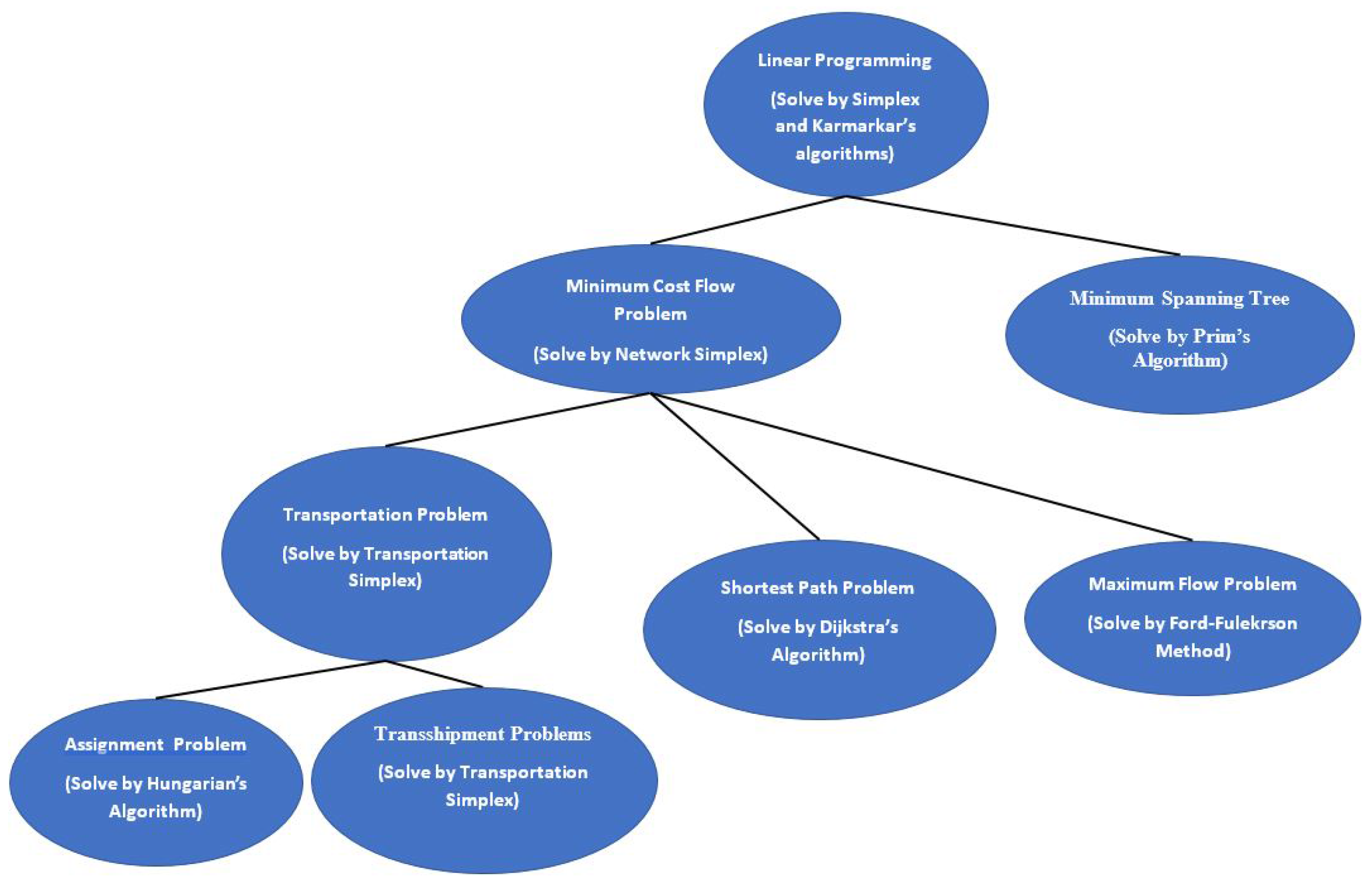
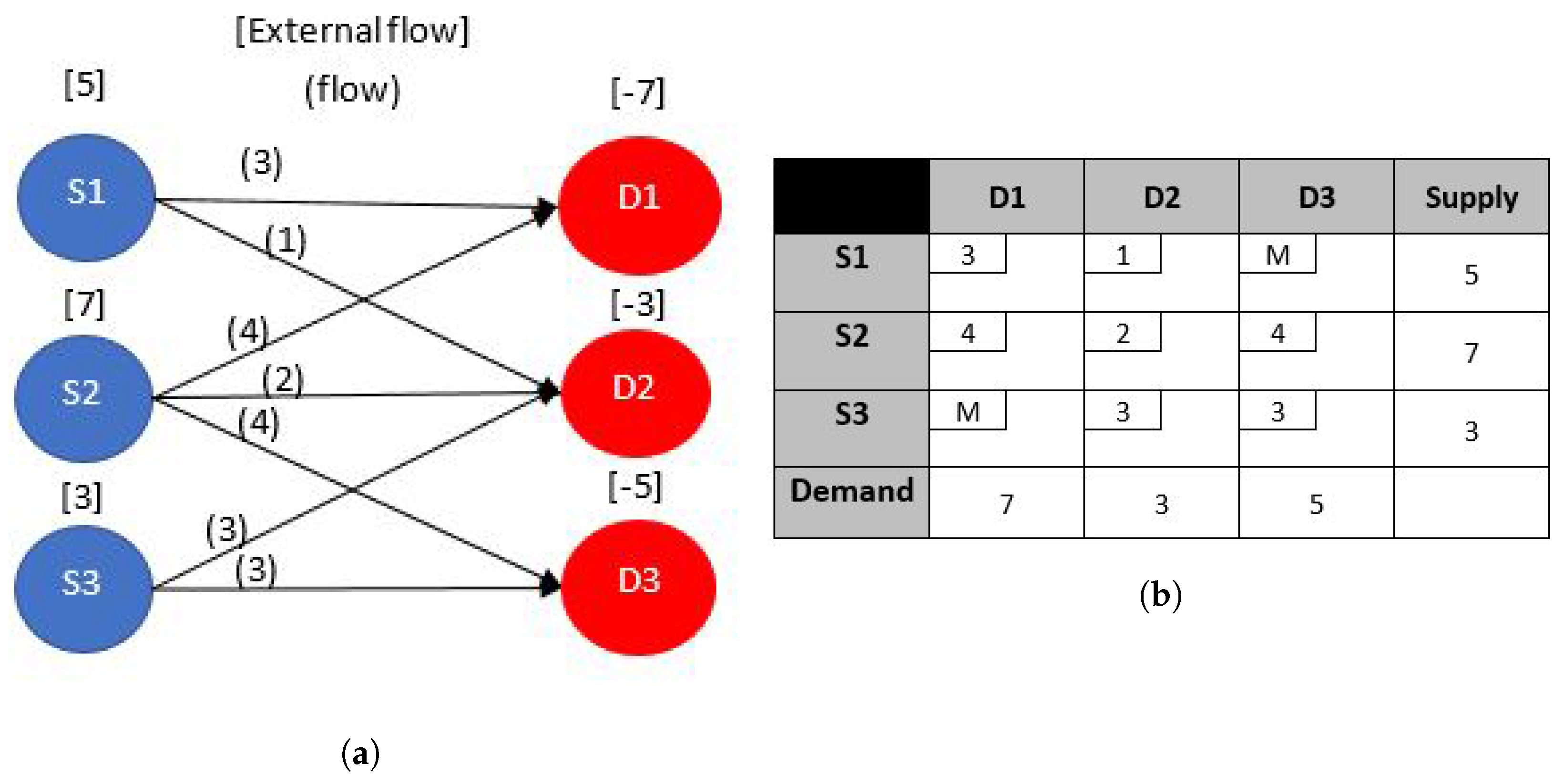

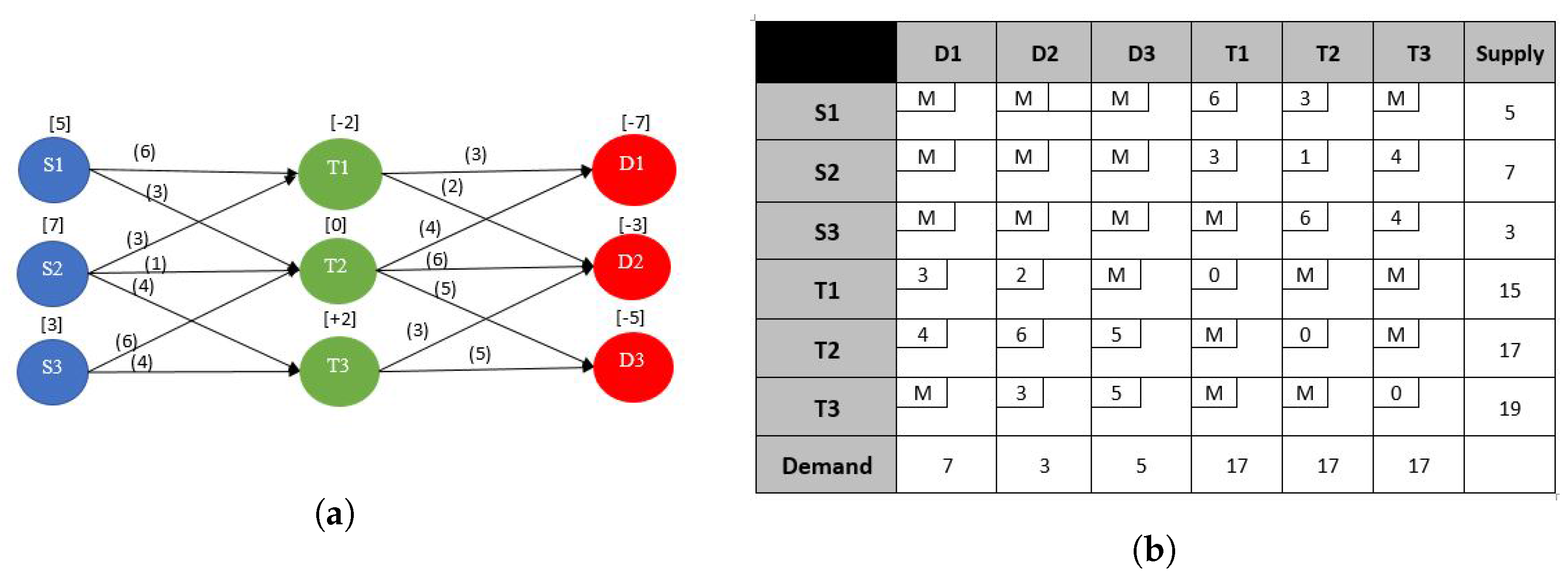
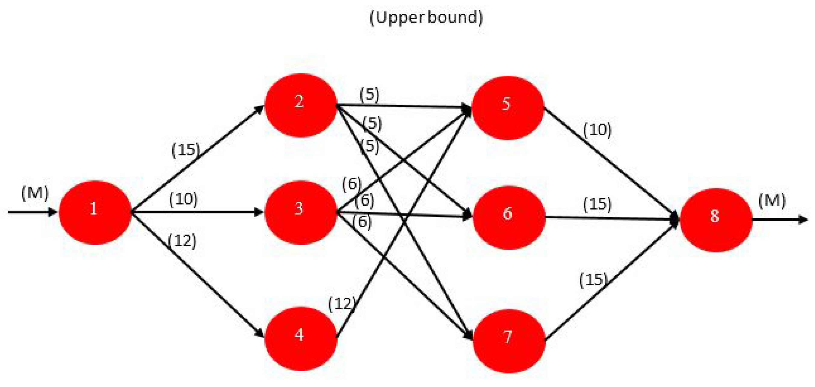
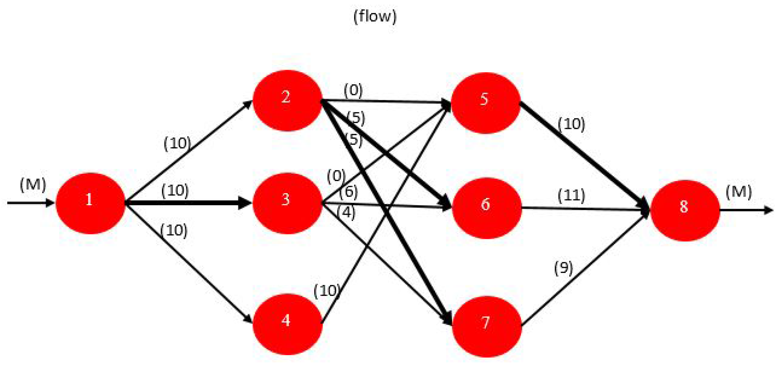


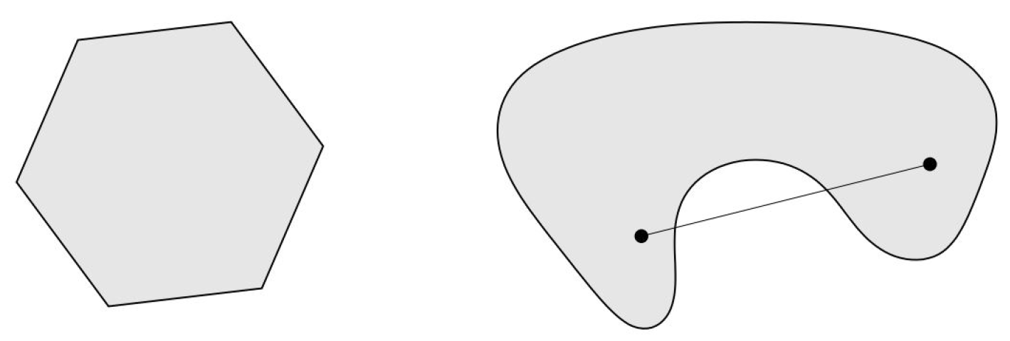


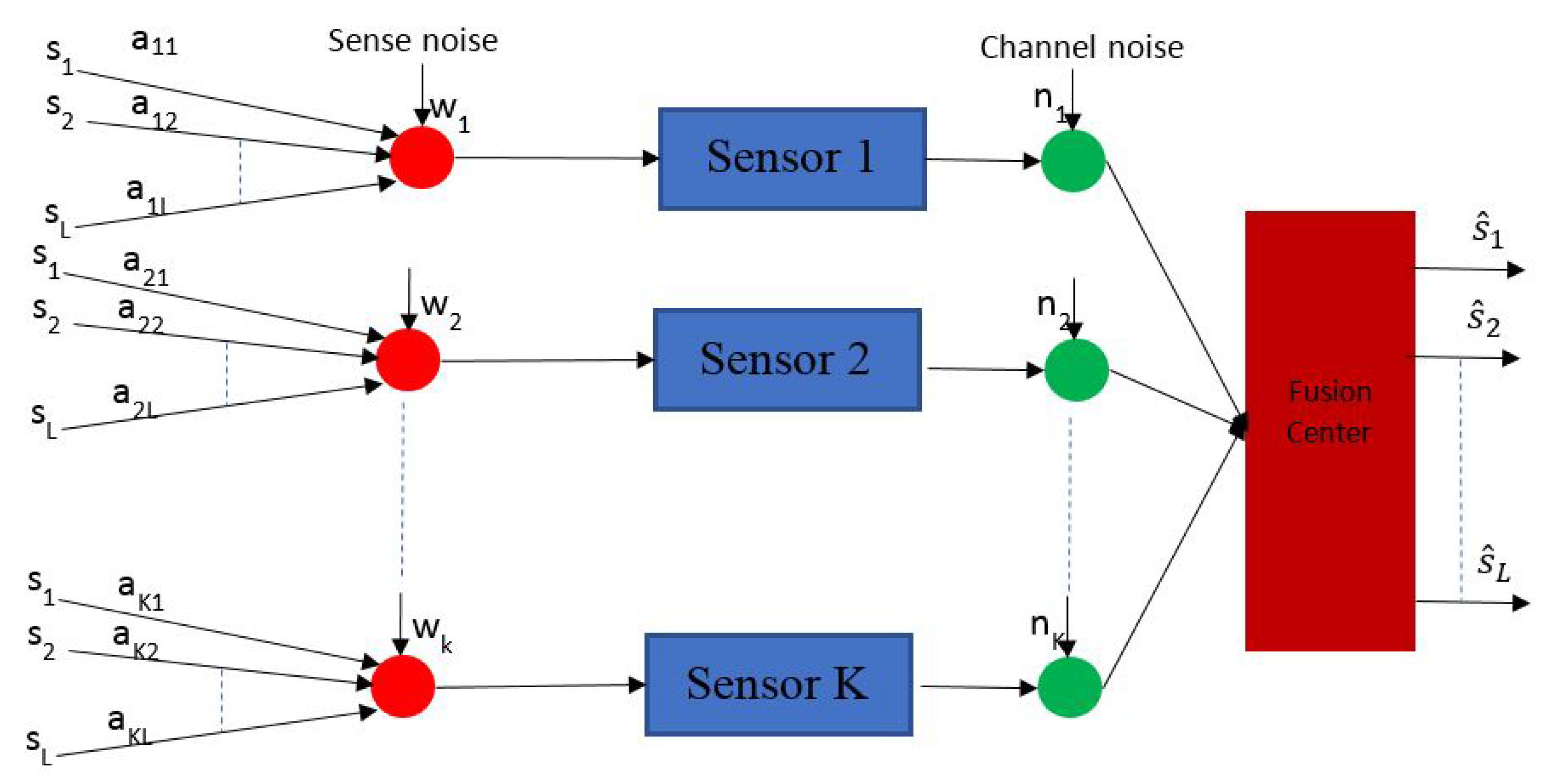

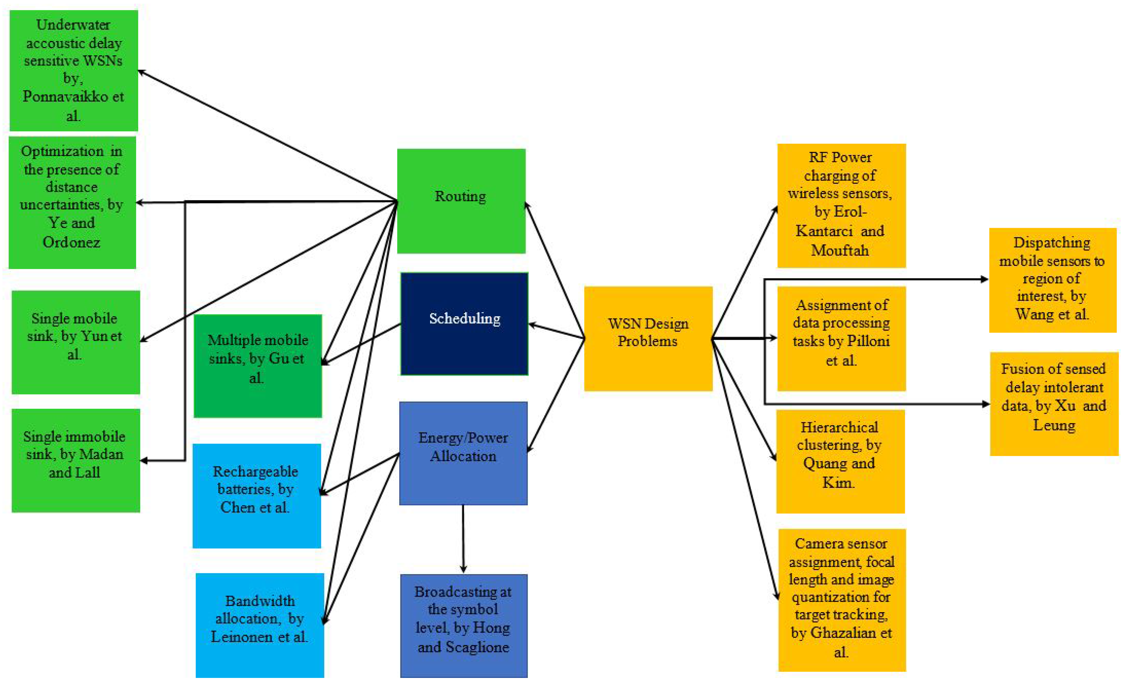
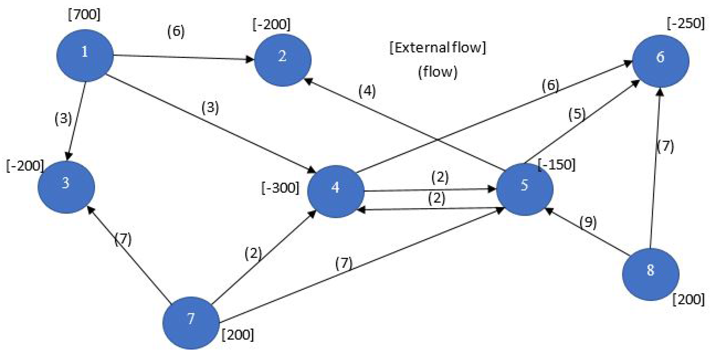
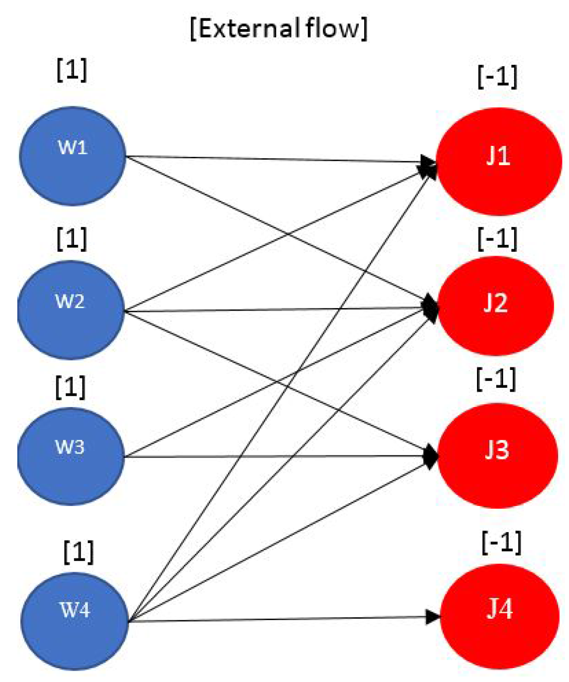
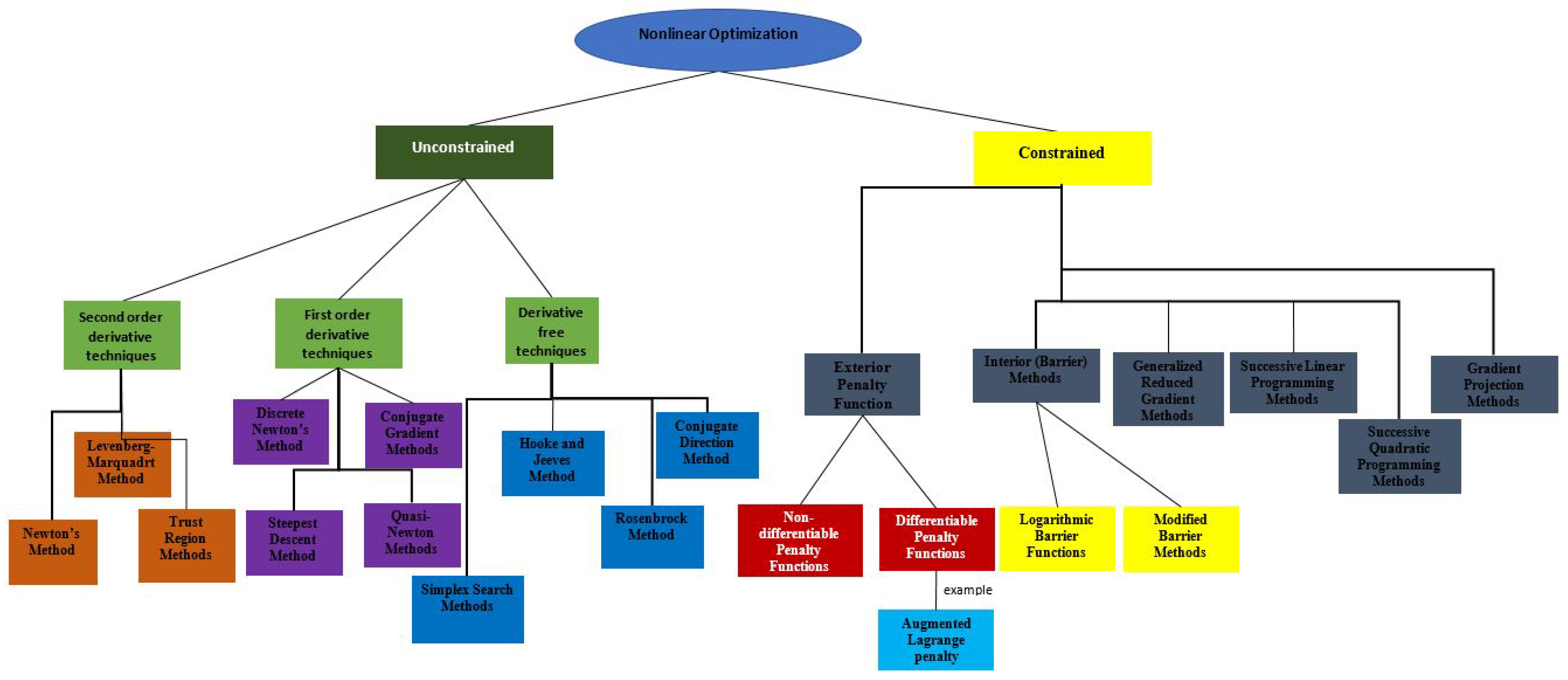
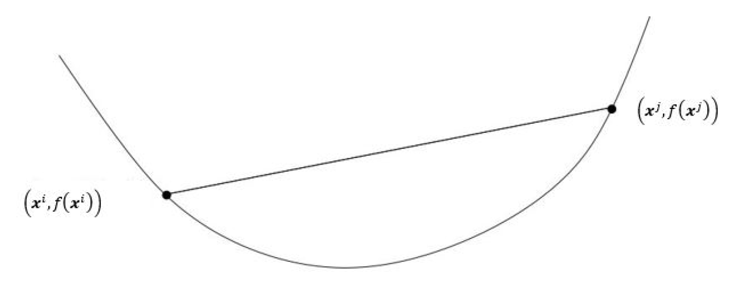
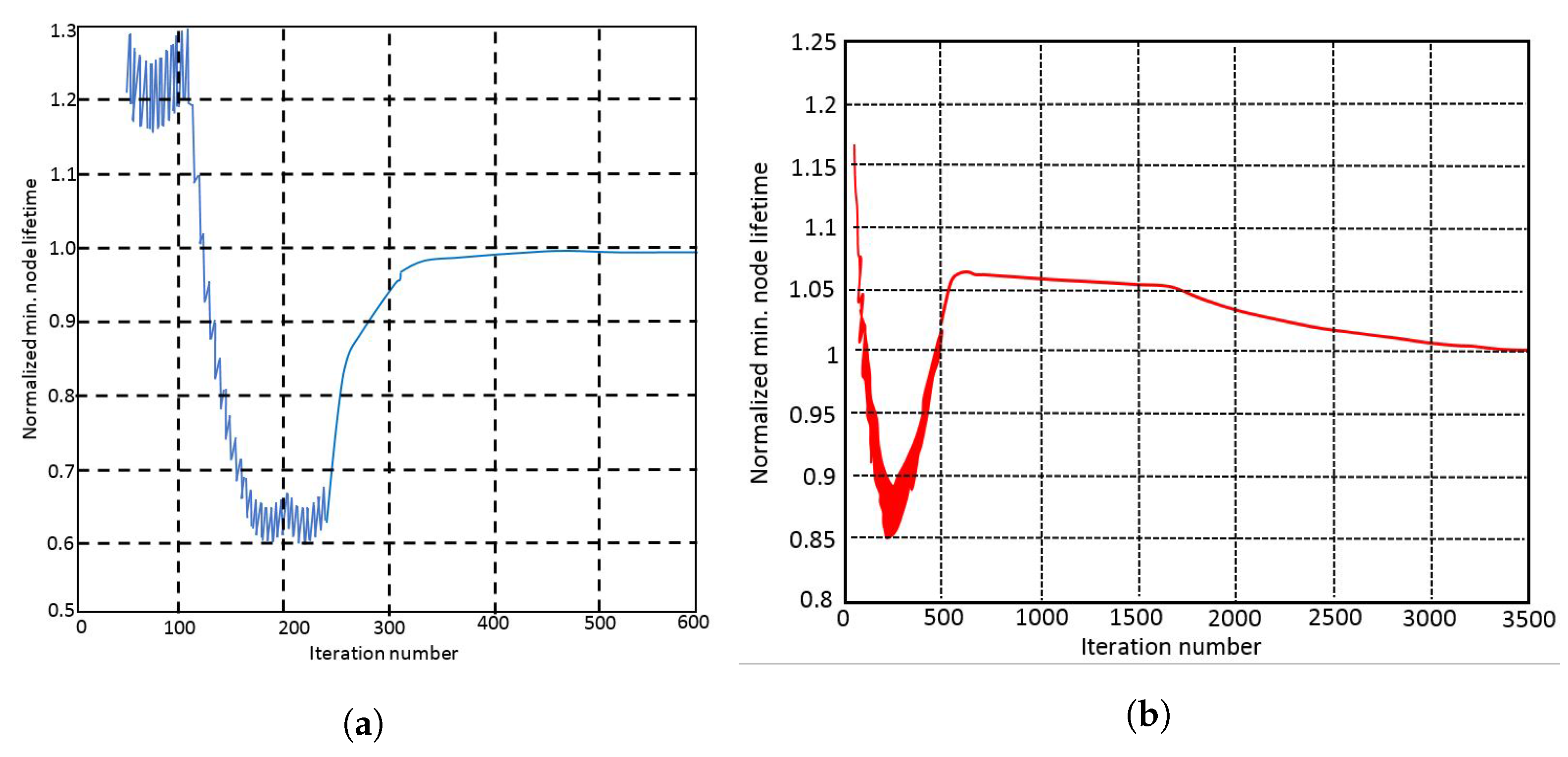
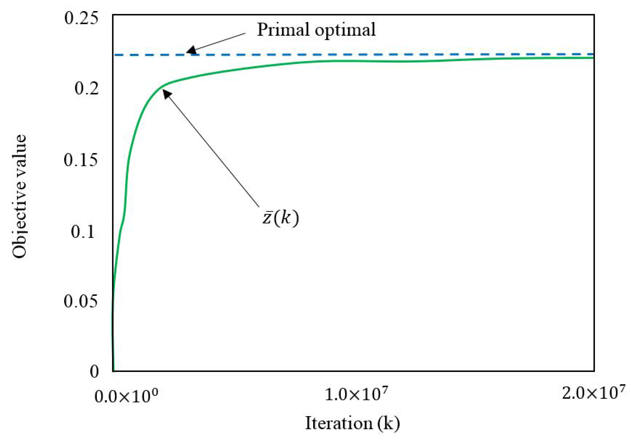
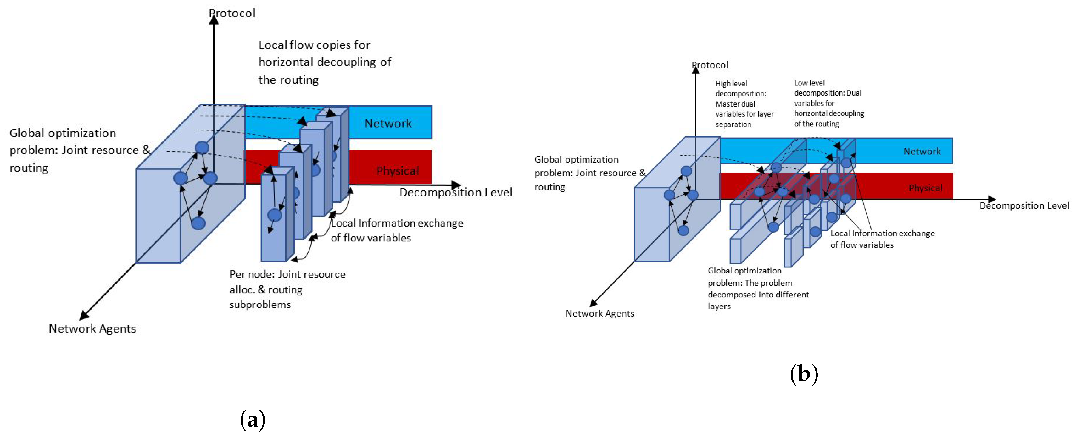
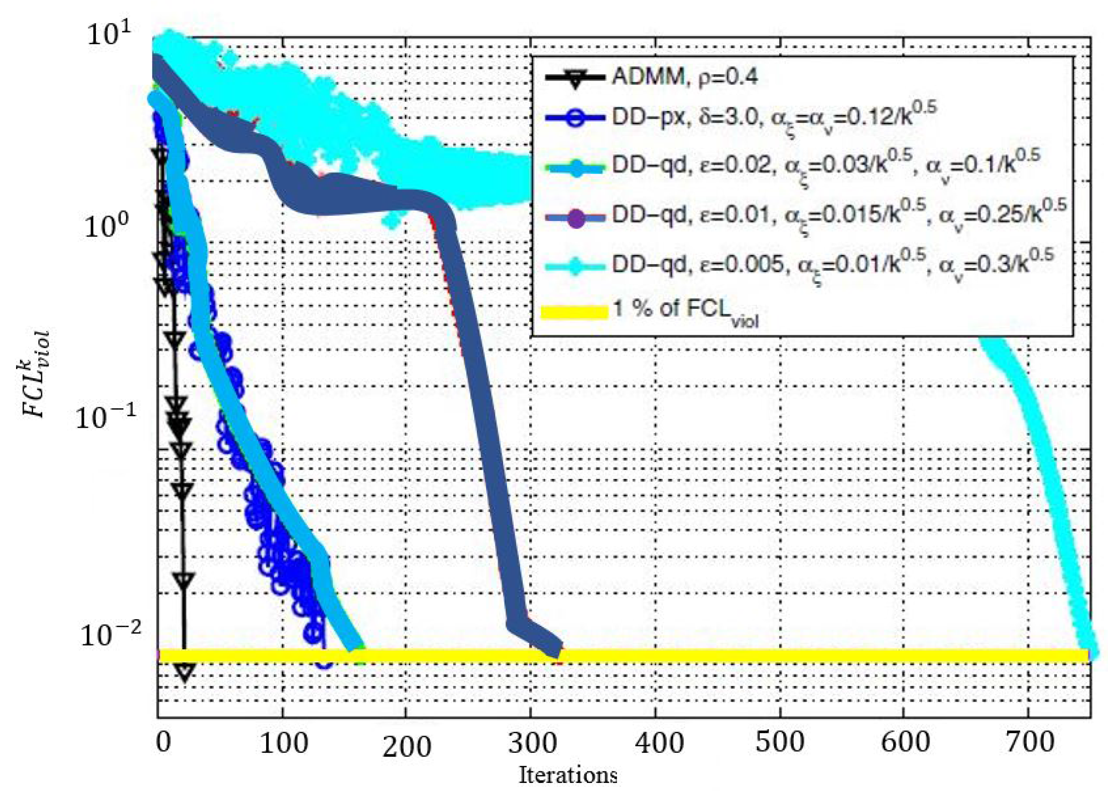
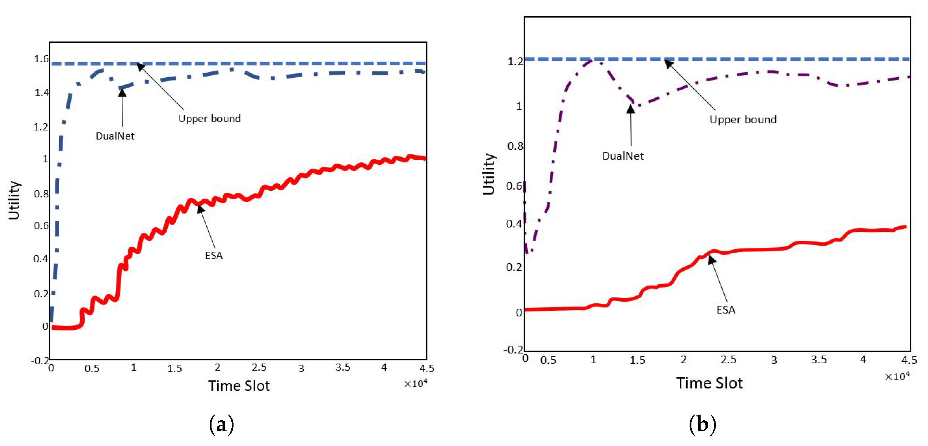
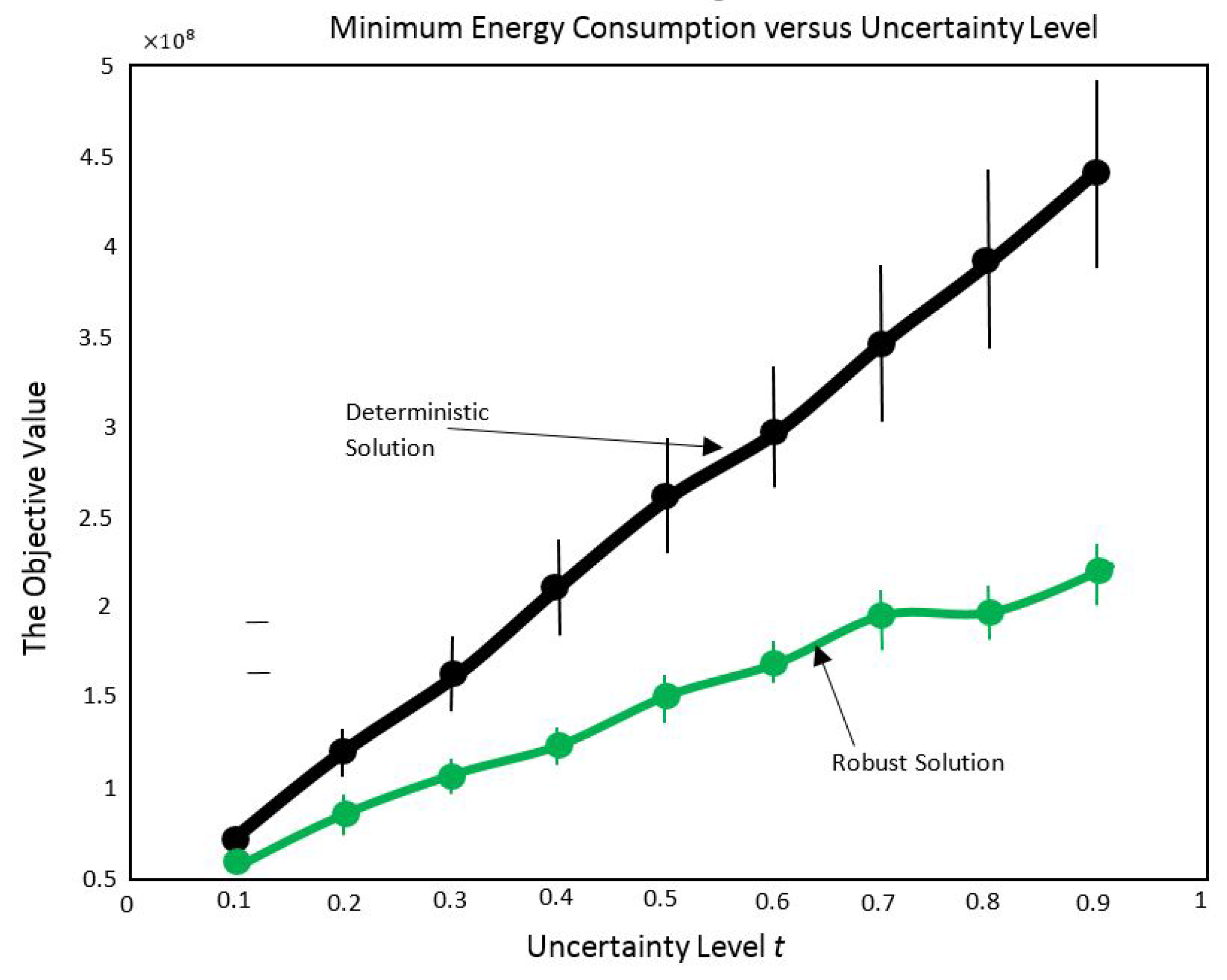
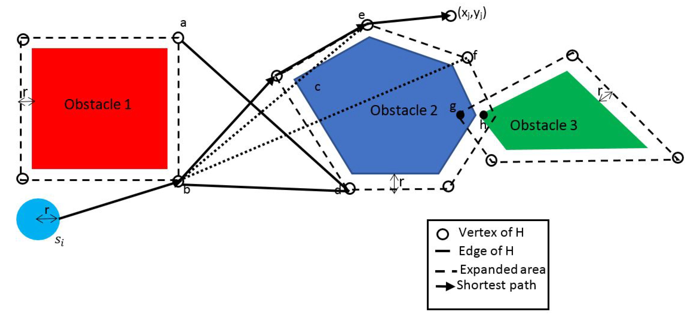
| Basic Variable | ||||||||||
|---|---|---|---|---|---|---|---|---|---|---|
| Row 0 | z | z = 0 | ||||||||
| Row 1 | ||||||||||
| Row 2 | ||||||||||
| Row 3 | ||||||||||
| Row 4 |
| Minimum Edge Weight Data Structure | Time Complexity |
|---|---|
| adjacency matrix, searching | |
| binary heap and adjacency list | |
| Fibonacci heap and adjacency list |
| Design Aspect | Classification of Initial Problem Formulation | Objective | Initial Problem Formulation: Centralized/Distributed? | Classification of Reformulated Problem | Solution Method | Implemented Solution Scheme for the Problem: Centralized/Distributed? | Nature of Solution | Convergence Speed/Complexity |
| Energy and route allocation from multiple source to multiple destination in rechargeable WSNs [5] | Complicated Convex NLP | Maximize Aggregate node utilities | Centralized | Decomposed to two easier strictly convex subproblems by decoupling the time component | Dual decomposition +subgradient algorithm used in a heuristic scheme | Distributed | suboptimal in finite time but optimal in infinite time | Too slow, took 5000 min to reach the best suboptimal solution in the simulations done in [5] |
| Joint Routing and TDMA scheduling for delay sensitive underwater acoustic WSNs [8] | NLP with general undetermined nonlinear term in the objective function | Minimize the transmission energy | Centralized | Mixed Integer Linear Program | Not stated, an MILP solver is assumed to have been used | Centralized | E Global optimal to the MILP but is suboptimal to the original NLP problem | Depends on the desired approximation error. Expected to be fast for large approximation errors but slow for small approximation errors, hence there is a trade-off. |
| Routing for a WSN Multi-hop with Single Immobile Sink [2] | bilinear quadratically constrained program | Maximizes the shortest lifetime across all nodes | Centralized |
| Dual Decomposition + subgradient algorithm |
| E Global Optimal |
|
| Joint Routing and Scheduling in WSNs with Multiple Sinks and Different Sink Location Possibilities [7] | Non -Linear and non-deterministic (due to the integration function) | Maximize the network lifetime | Centralized | Non-Linear Quadratically constrained Program | Column Generation Method | Centralized | Global Optimal | Too quick for small problems (less than one second and 6 iterations) but unknown for large problems |
| Dispatching of Mobile Sensor Nodes in a WSN to Sense a Particular Region of Interest [13] | Maximum-weight maximum-matching problem | Minimize the total expended motion energy | Centralized | N/A | Hungarian and Dijkstra’s algorithms | Centralized | Global Optimal | Cubic polynomial time complexity |
| A greedy problem specific heuristic | Distributed | Suboptimal | Not provided | |||||
| Fusion of delay sensitive noise perturbed data sensed by different nodes in a given cluster [14] | Non-linear Program with non-determinisitc objective function | Minimize the mean distortion of the measured data by the sensors | Centralized | N/A | Heuristics+ Newton’s Method | N/A | Suboptimal | Was not provided |
| Co-operative Broadcasting at the Symbol Level [12] | Linear Program | Minimize the aggregate transmission energy | Centralized | N/A | Heuristcs | N/A | Suboptimal | Not provided |
| Joint routing, power and bandwidth allocation in FDMA WSNs [4] | Non-strictly convex non-linear constrained program | Minimize the aggregate power for all network links | Centralized | Convex non-linear global consensus problem | Augmented Lagrangian +Alternating direction method of multipliers | Distributed among nodes | Global optimal | Fast, converged in 21 iterations of the ADMM algorithm |
| Strictly convex non-linear program (using proximal regularization) | Dual decomposition and projected subgradient algorithm | Distributed among nodes and decomposed in protocol layers | Global optimal | Slower than ADMM, converges in 133 iterations of the projected subgradient algorithm | ||||
| Assignment of processing tasks across the WSN [10] | Mixed binary linear program | Maximize the life time of the network (defined as the lifetime of the first node to die of exhausted battery) | Centralized | Mixed binary linear program local to each node and its neighbors | Heuristic that relies on gossiping to solve a local BILP at each node | Distributed | Suboptimal | Was not shown, however is expected to be quick if the density of the network is low (even for a large network) since the size of the local MILP problem for each node depends on the number of neighbors it has. |
| Routing in a delay-tolerant WSN to a Single Mobile Sink [3] | Quadratically Constrained Program | Maximize the number of cycles made by mobile sink | Centralized | Linear program | Lagrangian relaxation +subgradient algorithm, greedy algorithm for fractional knapsack problems+ trivial heuristic for box constrained linear program | Decentralized algorithm | Good Suboptimal. Global Solution is also attainable in a long time | Good suboptimal in few iterations (100-200) and global after too many iterations. |
| Hierarchical Clustering in a heterogeneous Network [11] | Mixed Binary Linear Program | Minimizes the maximum expended energy among nodes | Centralized | N/A | Branch and cut framework | Centralized | Could be solved to the desired degree of (1+ ) optimality. | Was not Shown |
| Maximize total received power by rechargeable sensor nodes in a smart grid from a mobile wireless charger [9] | Binary Linear Program | Maximizes the total received power of high priority nodes | Centralized | N/A | Not stated, CPLEX solver was used to solve the problem | Centralized | Global optimum | Was not shown. However is expected to be faster for low resolution discretization and vice versa |
| Account for uncertainties in the distance between sensor nodes [6] | Linear Program | Aggregate transmission and reception normalized energies | N/A |
| Interior point methods, CPLEX solver was used to solve the problem | N/A | Global optimum | Can be solved in polynomial time |
| Linear Program | Maximize the transmitted data to the sink | |||||||
| Bilinear Constrained Program | Maximize the network lifetime |
© 2017 by the authors. Licensee MDPI, Basel, Switzerland. This article is an open access article distributed under the terms and conditions of the Creative Commons Attribution (CC BY) license (http://creativecommons.org/licenses/by/4.0/).
Share and Cite
Ibrahim, A.; Alfa, A. Optimization Techniques for Design Problems in Selected Areas in WSNs: A Tutorial. Sensors 2017, 17, 1761. https://doi.org/10.3390/s17081761
Ibrahim A, Alfa A. Optimization Techniques for Design Problems in Selected Areas in WSNs: A Tutorial. Sensors. 2017; 17(8):1761. https://doi.org/10.3390/s17081761
Chicago/Turabian StyleIbrahim, Ahmed, and Attahiru Alfa. 2017. "Optimization Techniques for Design Problems in Selected Areas in WSNs: A Tutorial" Sensors 17, no. 8: 1761. https://doi.org/10.3390/s17081761
APA StyleIbrahim, A., & Alfa, A. (2017). Optimization Techniques for Design Problems in Selected Areas in WSNs: A Tutorial. Sensors, 17(8), 1761. https://doi.org/10.3390/s17081761