Control Measurements of Crane Rails Performed by Terrestrial Laser Scanning

 ,
,
Abstract
:1. Introduction
2. Measurement Method and Computations
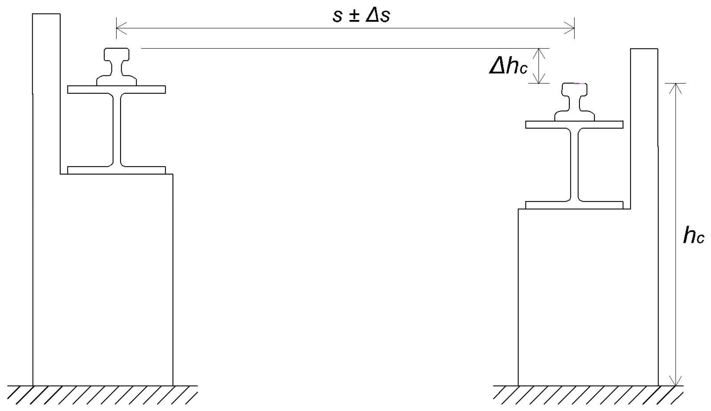
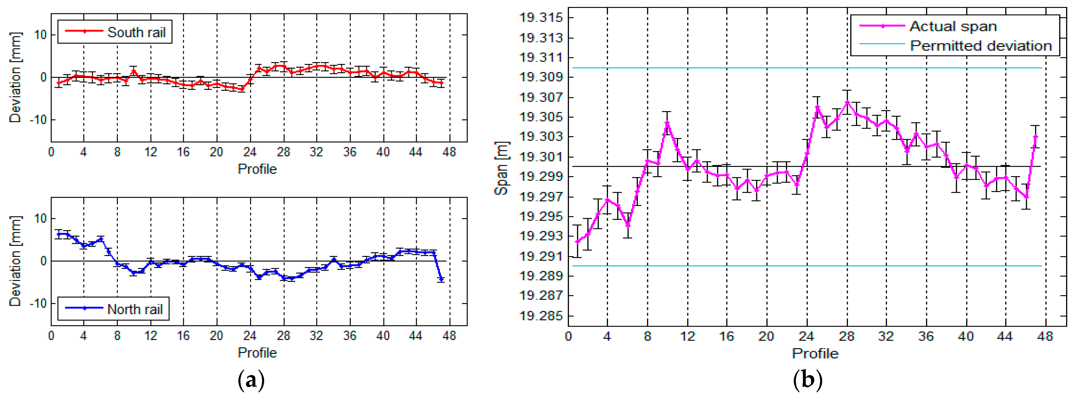
- the actual span can deviate from the projected span by a maximum of (Figure 1),
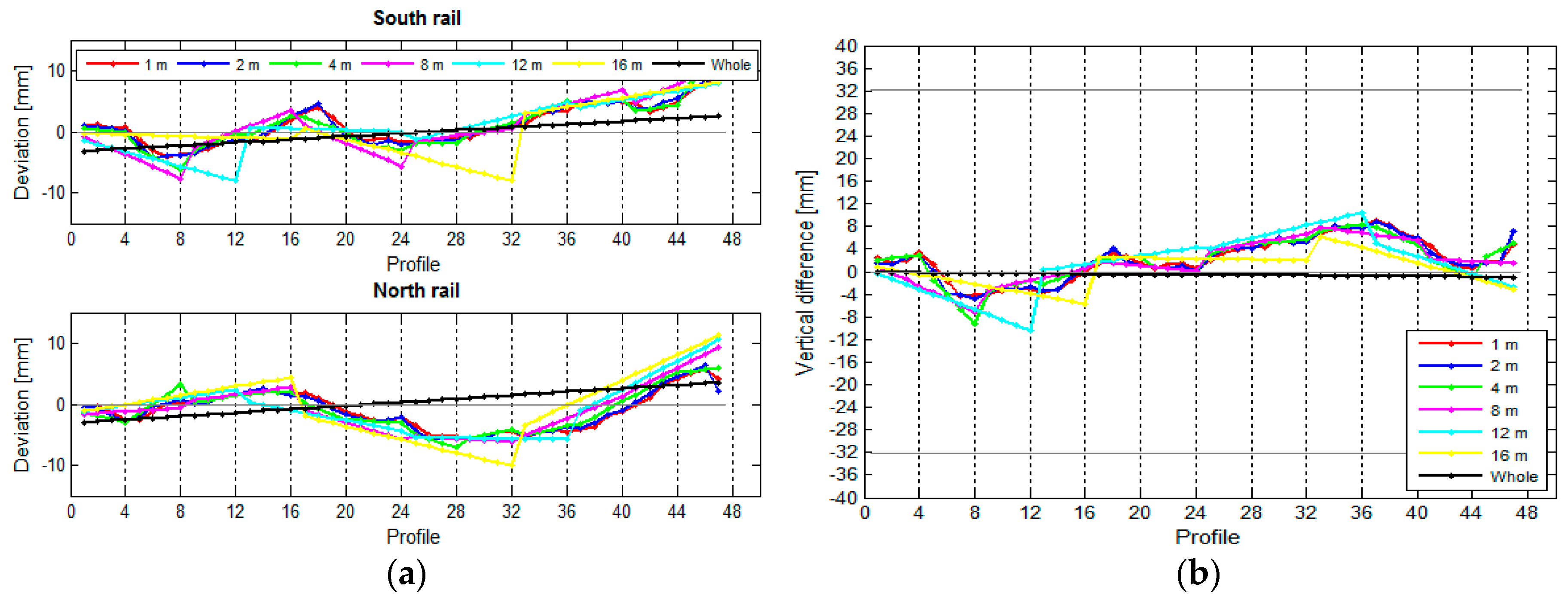
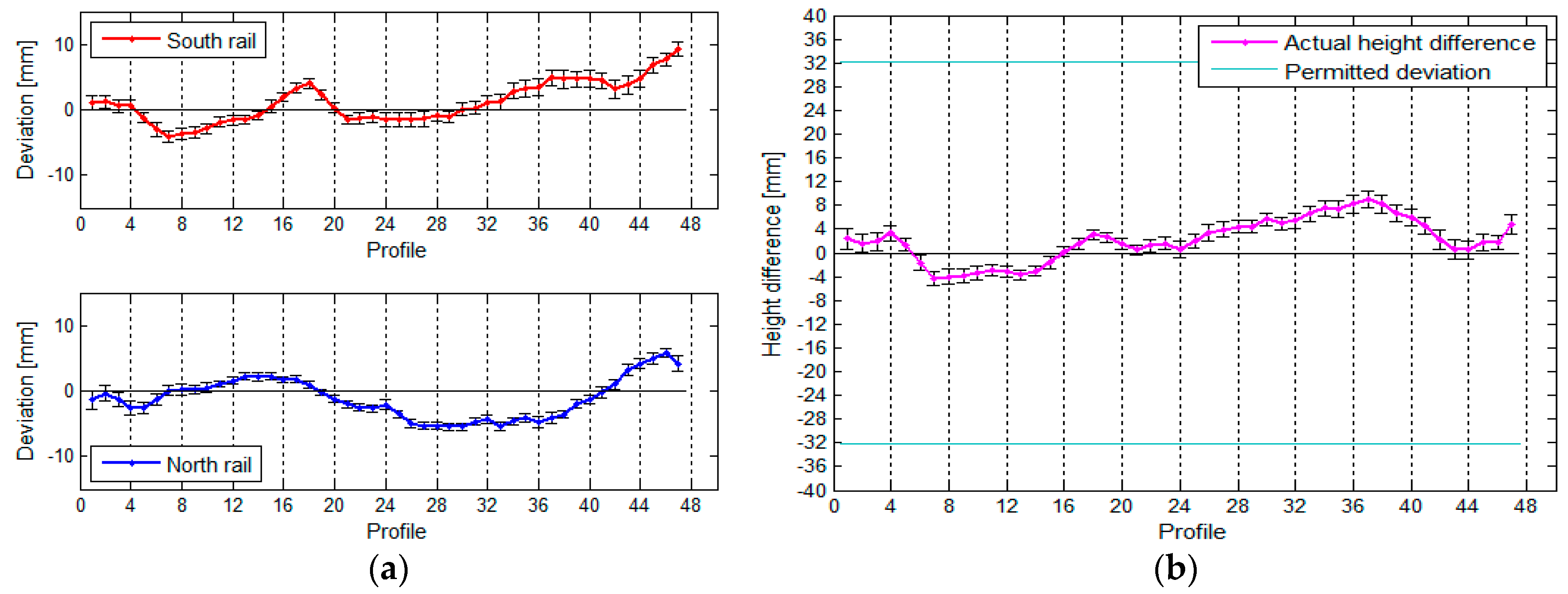
- the height difference between the rails within an individual cross section has to be in line with .
- alignment and geometric levelling,
- polar method with total station (TPS), and
- terrestrial laser scanning (TLS).
2.1. Measuring the Crane Rails in the Machine Room in the HPP in Krško
2.1.1. TPS Measurement of the Crane Rails
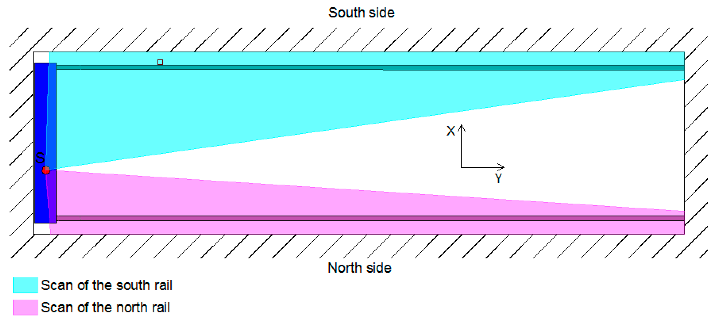
2.1.2. TLS Measurement of the Crane Rails
2.2. Crane Rail Measurements in the Gas Block Hall in the TPP in Brestanica
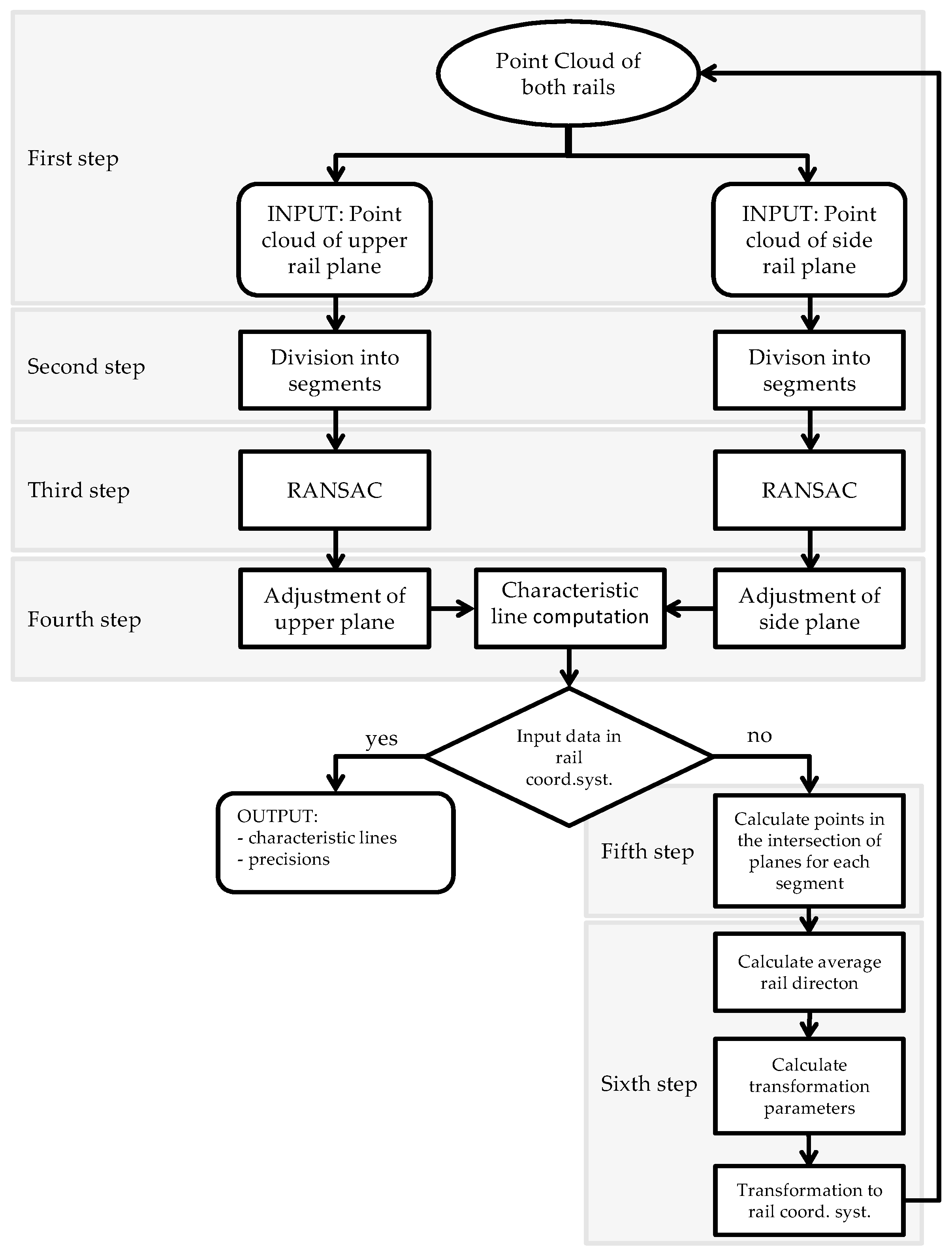
2.3. Treating the Point Clouds and Computing the Rail Parameters
2.3.1. Treating the Point Clouds and Calculating the Characteristic Rail Lines
2.3.2. The Computation of the Geometry of the Rails
3. Results and Analysis
3.1. Results: Spans and Height Differences
3.1.1. TPS Measurement of the Crane Rails in the HPP in Krško
3.1.2. TLS measurement of the crane rails in the HPP in Krško
3.1.3. TLS Measurement of the Crane Rails in the TPP in Brestanica
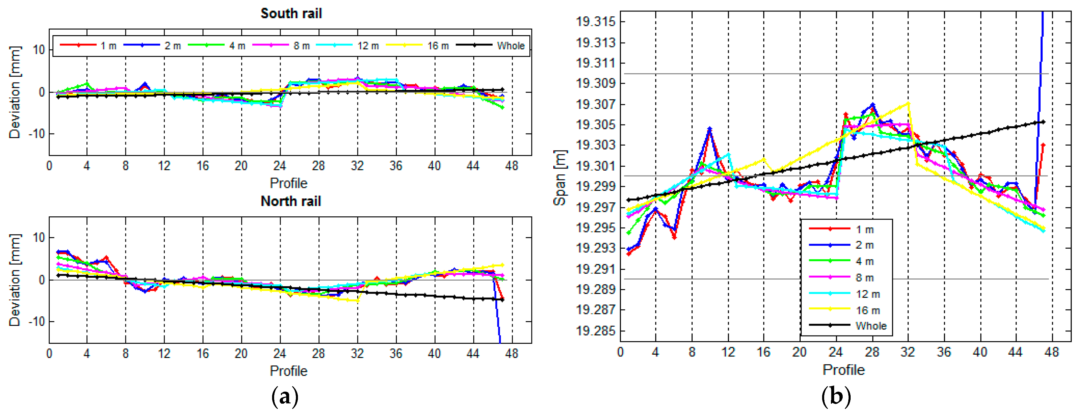
3.2. The Influence of Segment Length on the TLS Measurement Results
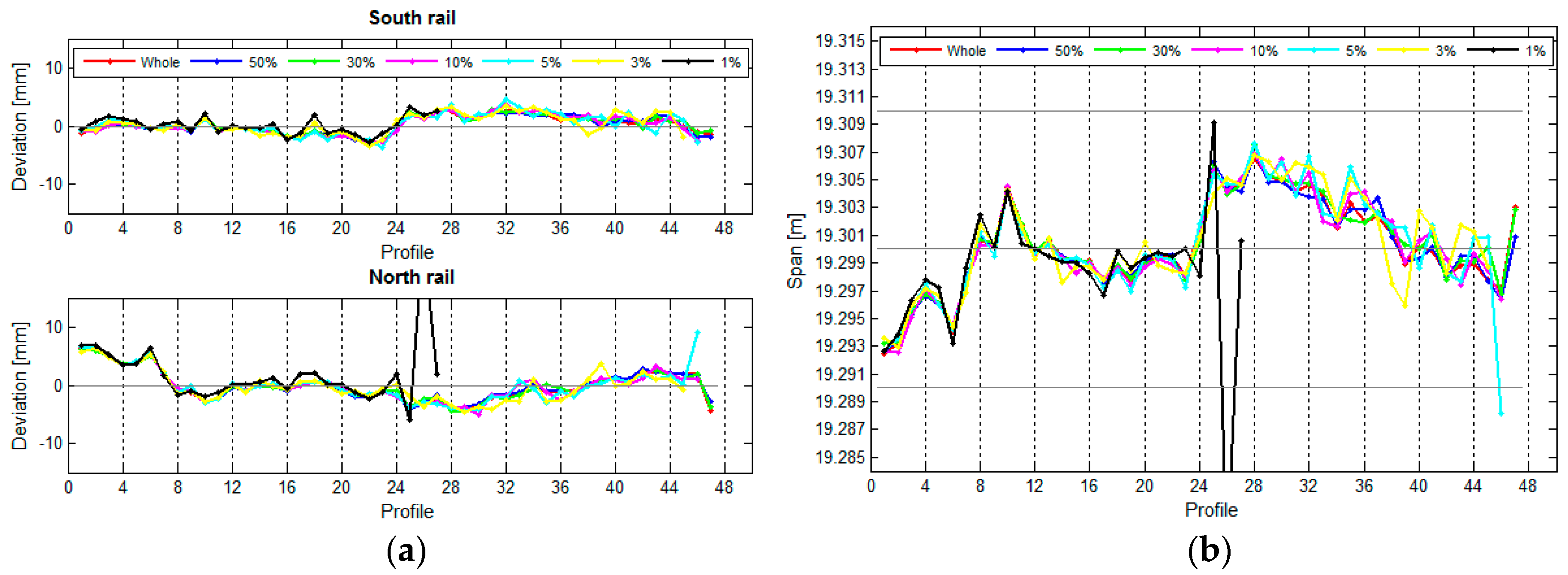
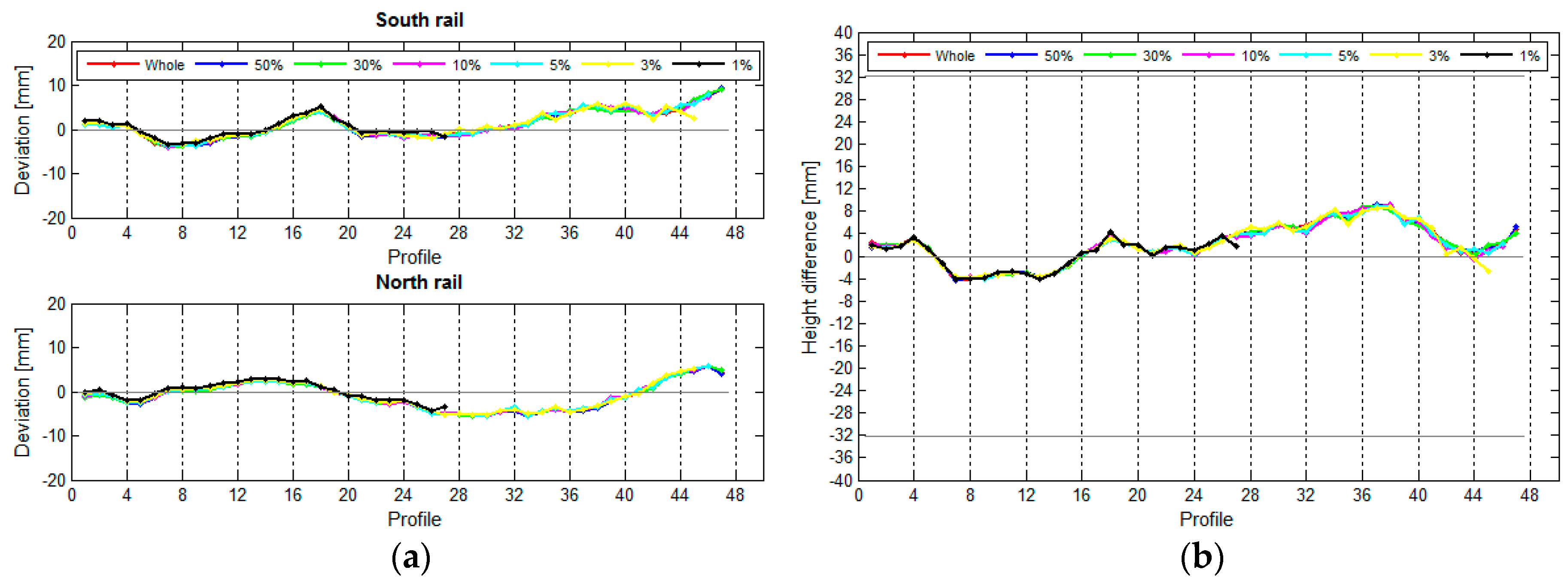
3.3. The Influence of the Density of Scanned Points on TLS Measurements
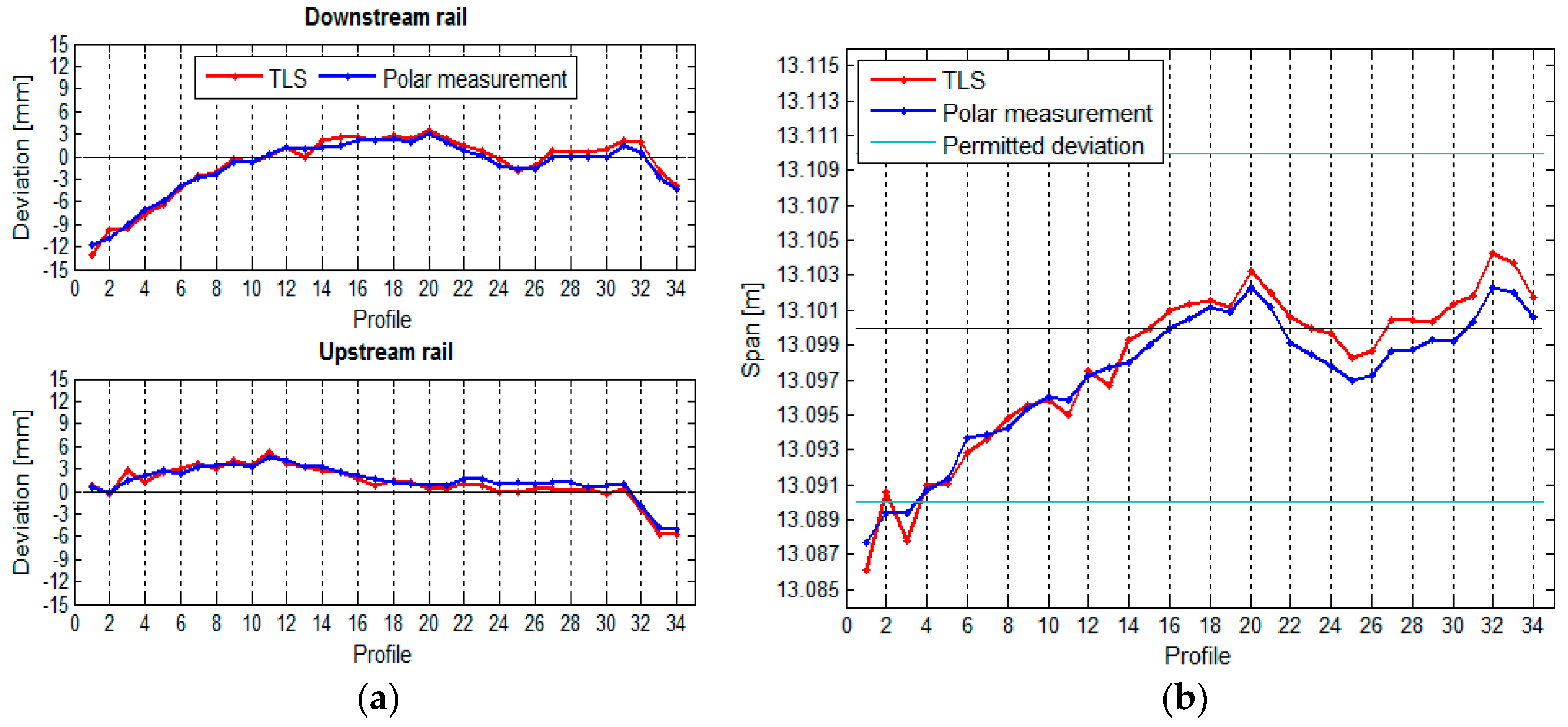
3.4. Comparison of TLS and TPS Measurements
4. Discussion and Conclusions
Acknowledgments
Author Contributions
Conflicts of Interest
References
- Vosselman, G.; Maas, H.G. Airborne and Terrestrial Laser Scanning, 1st ed.; Whittles Publishing: Dunbeath, UK, 2010. [Google Scholar]
- Shan, J.; Toth, C.K. Topographic Laser Ranging and Scanning: Principles and Processing; Taylor & Francis Group: Boca Raton, FL, USA, 2009. [Google Scholar]
- Babenko, P. Visual Inspection of Railroad Tracks. Ph.D. Thesis, College of Engineering and Computer Science, Orlando, FL, USA, 2009. Available online: http://etd.fcla.edu/CF/CFE0002895/Babenko_Pavel_200912_PhD.pdf (accessed on 17 July 2017).
- Benito, D.D. Automatic 3D Modelling of Train Rails in a LiDAR Point Cloud. Master’s Thesis, Faculty of Geo-Information Science and Earth Observation, Twente, The Netherlands, 2012. Available online: https://www.itc.nl/library/papers_2012/msc/gfm/diazbenito.pdf (accessed on 17 July 2017).
- Oude Elberink, S.; Khoshelham, K.; Arastounia, M.; Díaz Benito, D. Rail Track Detection and Modelling in Mobile Laser Scanner Data. ISPRS Ann. Photogramm. Remote Sens. Spat. Inform. Sci. 2013, 2, 223–228. [Google Scholar] [CrossRef]
- Soni, A.; Robson, S.; Gleeson, B. Extracting Rail Track Geometry from Static Terrestrial Laser Scans for Monitoring Purposes. Int. Arch. Photogramm. Remote Sens. Spat. Inform. Sci. 2014, 5, 553. [Google Scholar] [CrossRef]
- Soni, A.; Robson, S.; Gleeson, B. Optical Non-Contact Railway Track Measurement with Static Terrestrial Laser Scanning to Better Than 1.5 mm RMS. In Proceedings of the FIG Working Week 2015, From the Wisdom of the Ages to the Challenges of the Modern World, Sofia, Bulgaria, 17–21 May 2015; pp. 1–15. [Google Scholar]
- Kopáčik, A.; Wunderlich, T.A. Usage of Laser Scanning Systems at Hydro-technical Structures. In Proceedings of the FIG Working Week 2004, Athens, Greece, 22–27 May 2004; pp. 1–8. Available online: https://www.fig.net/resources/proceedings/fig_proceedings/athens/papers/ts23/TS23_4_Kopacik_Wunderlich.pdf (accessed on 17 July 2017).
- Erdélyi, J.; Kopáčik, A.; Lipták, I.; Kyrinovič, P. Suspended steel bridge monitoring using terrestrial laser scanning. Int. J. Interdiscip. Theory Pract. 2016, 8, 107–111. [Google Scholar]
- Erdélyi, J.; Kopáčik, A.; Lipták, I.; Kyrinovič, P. Pedestrian bridge monitoring using terrestrial laser scanning. In Advances and Trends in Engineering Sciences and Technologies; Ali, M.A., Platko, P., Eds.; Taylor & Francis Group: London, UK, 2016; pp. 51–56. [Google Scholar]
- Kyrinovič, P.; Kopáčik, A. Automated measurement system for crane rail geometry determination. In Proceedings of the 27th ISARC, Bratislava, Slovakia, 25–27 June 2010; pp. 249–305. [Google Scholar]
- Erdélyi, J.; Kopáčik, A.; Lipták, I.; Kyrinovič, P. Automation of point cloud processing to increase the deformation monitoring accuracy. Appl. Geomat. 2017, 9, 105–113. [Google Scholar] [CrossRef]
- Kŕemen, T.; Koska, B.; Pospíšil, J.; Kyrinovič, P.; Haličková, J.; Kopáčik, A. Checking of Crane Rails by Terrestrial Laser Scanning Technology. In Proceedings of the 13th FIG Symposium on Deformation Measurement and Analysis and 4th IAG Symposium on Geodesy for Geotechnical and Structural Engineering, Lisbon, Portugal, 12–15 May 2008; pp. 12–15. [Google Scholar]
- Kostov, G.P. Application, Specifics and Technical Implementation of the 3D Terrestrial Laser Scanning for Measurement and Analysis of the Spatial Geometry of a Steel Construction. In Proceedings of the FIG Working Week 2015, From the Wisdom of the Ages to the Challenges of the Modern World, Sofia, Bulgaria, 17–21 May 2015; pp. 1–15. [Google Scholar]
- Cabaleiro, M.; Riveiro, B.; Arias, P.; Caamaño, J.C. Algorithm for Beam Deformation Modelling from LiDAR Data. Measurement 2015, 76, 20–31. [Google Scholar] [CrossRef]
- de Asís López, F.; García-Cortés, S.; Roca-Pardiñas, J.; Ordóñez, C. Geometric Optimization of Trough Collectors Using Terrestrial Laser Scanning: Feasibility Analysis Using a New Statistical Assessment Method. Measurement 2014, 47, 92–99. [Google Scholar] [CrossRef]
- EUROCODE 3-Design of Steel Structures-Part 6: Crane Supporting Structures. Available online: https://law.resource.org/pub/eu/eurocode/en.1993.6.2007.pdf (accessed on 17 July 2017).
- Kovanič, L.; Gašinec, J.; Kovanič, L.; Lechman, P. Geodetic Surveying of Crane Trail Space Relations. Acta Montan. Slovaca 2010, 1, 188–199. Available online: http://actamont.tuke.sk/pdf/2010/n3/03_Gasinec.pdf (accessed on 17 July 2017).
- Marjetič, A.; Kregar, K.; Ambrožič, T.; Kogoj, D. An Alternative Approach to Control Measurements of Crane Rails. Sensors 2012, 12, 5906–5918. [Google Scholar] [CrossRef] [PubMed]
- Lemmens, M. Geo-Information, Technologies, Applications and the Environment; Springer: New York, NY, USA, 2011. [Google Scholar] [CrossRef]
- Derpanis, K.G. Overview of the RANSAC Algorithm. Image Rochester NY 2010, 4, 2–3. [Google Scholar]
- Urbančič, T.; Vrečko, A.; Kregar, K. The Reliability of the RANSAC Method when Estimating the Parameters of a Geometric Object. Geodetski Vestnik 2016, 60, 69–97. [Google Scholar] [CrossRef]
- Pearson, K.L., III. On Lines and Planes of Closest Fit to Systems of Points in Space. Lond. Edinb. Dublin Philos. Mag. J. Sci. 1901, 2, 559–572. [Google Scholar] [CrossRef]


| Point | x [m] | y [m] | H [m] | [mm] | [mm] | [mm] |
|---|---|---|---|---|---|---|
| A | 1010.4798 | 989.7332 | 100.5468 | 0.1 | 0.1 | 0.5 |
| B | 949.7709 | 1012.4671 | 101.2770 | 0.1 | 0.1 | 0.3 |
| C | 955.9898 | 1022.4994 | 101.3517 | 0.1 | 0.1 | 0.3 |
| Rail | [mm] | [mm] | [mm] | [mm] |
|---|---|---|---|---|
| Downstream rail | 0.6 | 0.8 | 0.8 | 1.1 |
| Upstream rail | 0.5 | 0.8 |
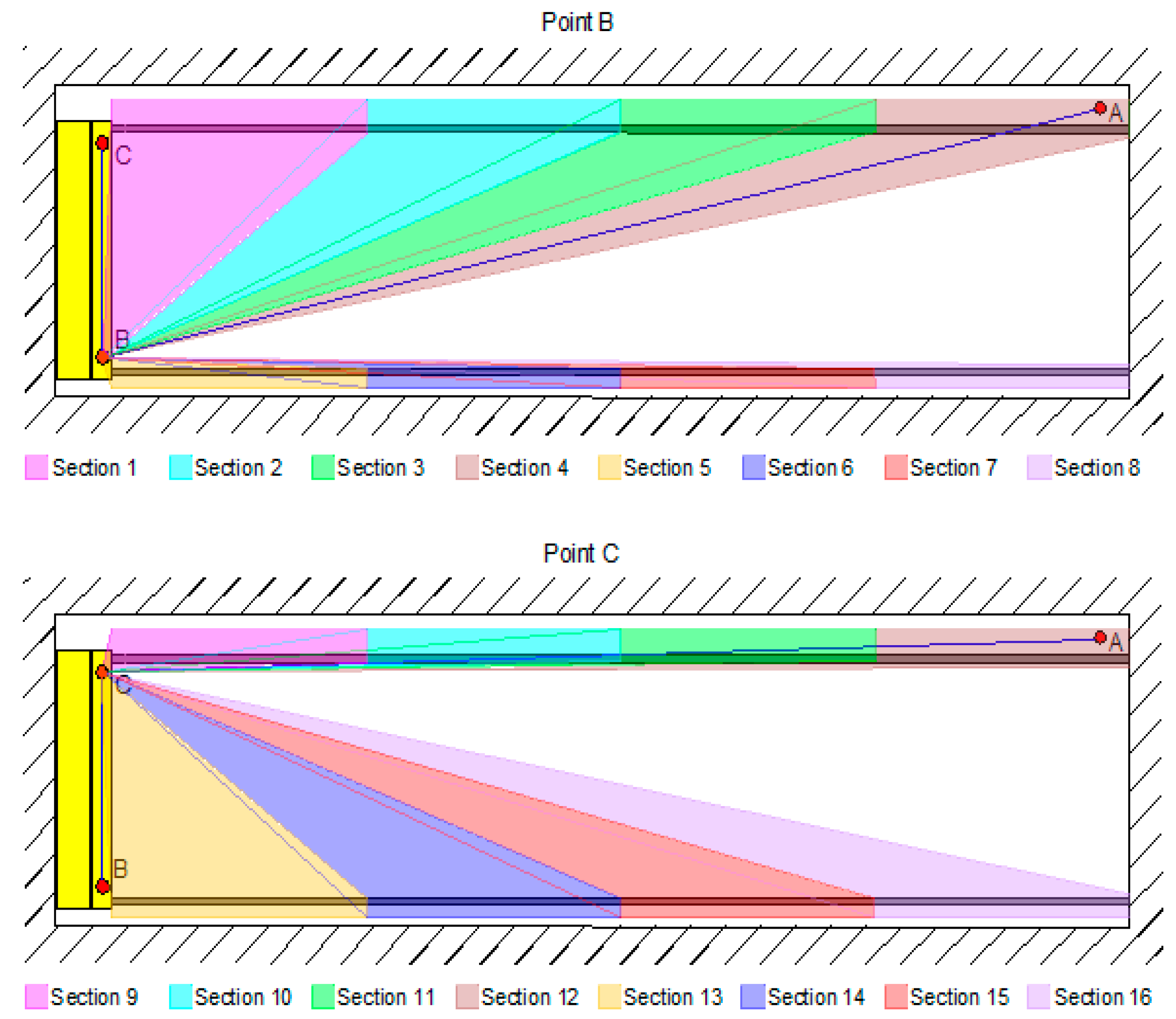
| Section | Horizontal Angular Grid [gon] | Vertical Angular Grid [gon] | Number of Captured Points | Scanning Time [min] |
|---|---|---|---|---|
| Point B | ||||
| 1 | 0.0445 | 0.0089 | 120,537 | 9 |
| 2 | 0.0207 | 0.0041 | 78,849 | 6 |
| 3 | 0.0126 | 0.0025 | 41,731 | 3 |
| 4 | 0.0113 | 0.0023 | 35,585 | 3 |
| 5 | 0.0053 | 0.0400 | 185,645 | 12 |
| 6 | 0.0053 | 0.0053 | 85,311 | 3 |
| 7 | 0.0445 | 0.0445 | 46,285 | 3 |
| 8 | 0.0106 | 0.0106 | 63,406 | 3 |
| Point C | ||||
| 9 | 0.0646 | 0.0129 | 83,791 | 3 |
| 10 | 0.0192 | 0.0038 | 13,382 | 1 |
| 11 | 0.0127 | 0.0025 | 12,105 | 1 |
| 12 | 0.0285 | 0.0057 | 5592 | 1 |
| 13 | 0.0430 | 0.0086 | 66,857 | 6 |
| 14 | 0.0273 | 0.0055 | 72,238 | 6 |
| 15 | 0.0187 | 0.0037 | 55,157 | 3 |
| 16 | 0.0110 | 0.0022 | 48,617 | 3 |
| % of Subsampled Points | 50% | 30% | 10% | 5% | 3% | 1% | ||||||
|---|---|---|---|---|---|---|---|---|---|---|---|---|
| Rail | S | N | S | N | S | N | S | N | S | N | S | N |
| Positional deviations | ||||||||||||
| Max. [mm] | 0.9 | 1.7 | 1.3 | 1.4 | 1.5 | 1.8 | 2.5 | 7.2 | 2.9 | 2.4 | 2.8 | 26.7 |
| No. of diff. >1.0 mm | 0 | 1 | 2 | 1 | 2 | 3 | 12 | 6 | 9 | 10 | 5 | 10 |
| No. of profiles | 47 | 47 | 47 | 47 | 46 | 46 | 46 | 46 | 45 | 45 | 27 | 27 |
| Aver. [mm] | 0.2 | 0.3 | 0.3 | 0.3 | 0.3 | 0.4 | 0.7 | 0.6 | 0.6 | 0.7 | 0.7 | 2.0 |
| ±St. dev. [mm] | ±0.2 | ±0.3 | ±0.3 | ±0.3 | ±0.3 | ±0.4 | ±0.6 | ±1.1 | ±0.6 | ±0.7 | ±0.6 | ±5.0 |
| Vertical deviations | ||||||||||||
| Max. [mm] | 0.6 | 0.8 | 1.1 | 0.8 | 1.2 | 0.7 | 1.1 | 0.7 | 4.1 | 1.1 | 1.3 | 1.8 |
| No. of diff. >1.0 mm | 0 | 0 | 1 | 0 | 1 | 0 | 1 | 0 | 3 | 1 | 4 | 2 |
| No. of profiles | 47 | 47 | 47 | 47 | 46 | 46 | 46 | 46 | 45 | 45 | 27 | 27 |
| Aver. [mm] | 0.1 | 0.1 | 0.2 | 0.1 | 0.3 | 0.2 | 0.2 | 0.2 | 0.6 | 0.4 | 0.7 | 0.7 |
| ±St. dev. [mm] | ±0.2 | ±0.1 | ±0.3 | ±0.1 | ±0.3 | ±0.2 | ±0.2 | ±0.2 | ±0.6 | ±0.2 | ±0.3 | ±0.3 |
| Comparison of the Downstream Rail Deviation | Comparison of the Upstream Rail Deviation | Comparison of the Span and Vertical Differences | ||||
|---|---|---|---|---|---|---|
| [mm] | [mm] | [mm] | [mm] | [mm] | [mm] | |
| Max. | 1.4 | 4.5 | 1.3 | 5.9 | 2.2 | 2.4 |
| Min. | 0.0 | 0.0 | 0.1 | 0.1 | 0.2 | 0.0 |
| Ave. | 0.6 | 1.8 | 0.6 | 2.5 | 1.1 | 1.1 |
© 2017 by the authors. Licensee MDPI, Basel, Switzerland. This article is an open access article distributed under the terms and conditions of the Creative Commons Attribution (CC BY) license (http://creativecommons.org/licenses/by/4.0/).
Share and Cite
Kregar, K.; Možina, J.; Ambrožič, T.; Kogoj, D.; Marjetič, A.; Štebe, G.; Savšek, S. Control Measurements of Crane Rails Performed by Terrestrial Laser Scanning. Sensors 2017, 17, 1671. https://doi.org/10.3390/s17071671
Kregar K, Možina J, Ambrožič T, Kogoj D, Marjetič A, Štebe G, Savšek S. Control Measurements of Crane Rails Performed by Terrestrial Laser Scanning. Sensors. 2017; 17(7):1671. https://doi.org/10.3390/s17071671
Chicago/Turabian StyleKregar, Klemen, Jan Možina, Tomaž Ambrožič, Dušan Kogoj, Aleš Marjetič, Gašper Štebe, and Simona Savšek. 2017. "Control Measurements of Crane Rails Performed by Terrestrial Laser Scanning" Sensors 17, no. 7: 1671. https://doi.org/10.3390/s17071671
APA StyleKregar, K., Možina, J., Ambrožič, T., Kogoj, D., Marjetič, A., Štebe, G., & Savšek, S. (2017). Control Measurements of Crane Rails Performed by Terrestrial Laser Scanning. Sensors, 17(7), 1671. https://doi.org/10.3390/s17071671