Multisensor Parallel Largest Ellipsoid Distributed Data Fusion with Unknown Cross-Covariances

_Zhu.png)
Abstract
:1. Introduction
2. Preliminaries
3. Distributed Fusion Algorithms
3.1. Optimal Distributed Kalman Fuser Weighted by Matrices
3.2. Largest Ellipsoid Fusion Algorithm
4. Multisensor Largest Ellipsoid Fusers
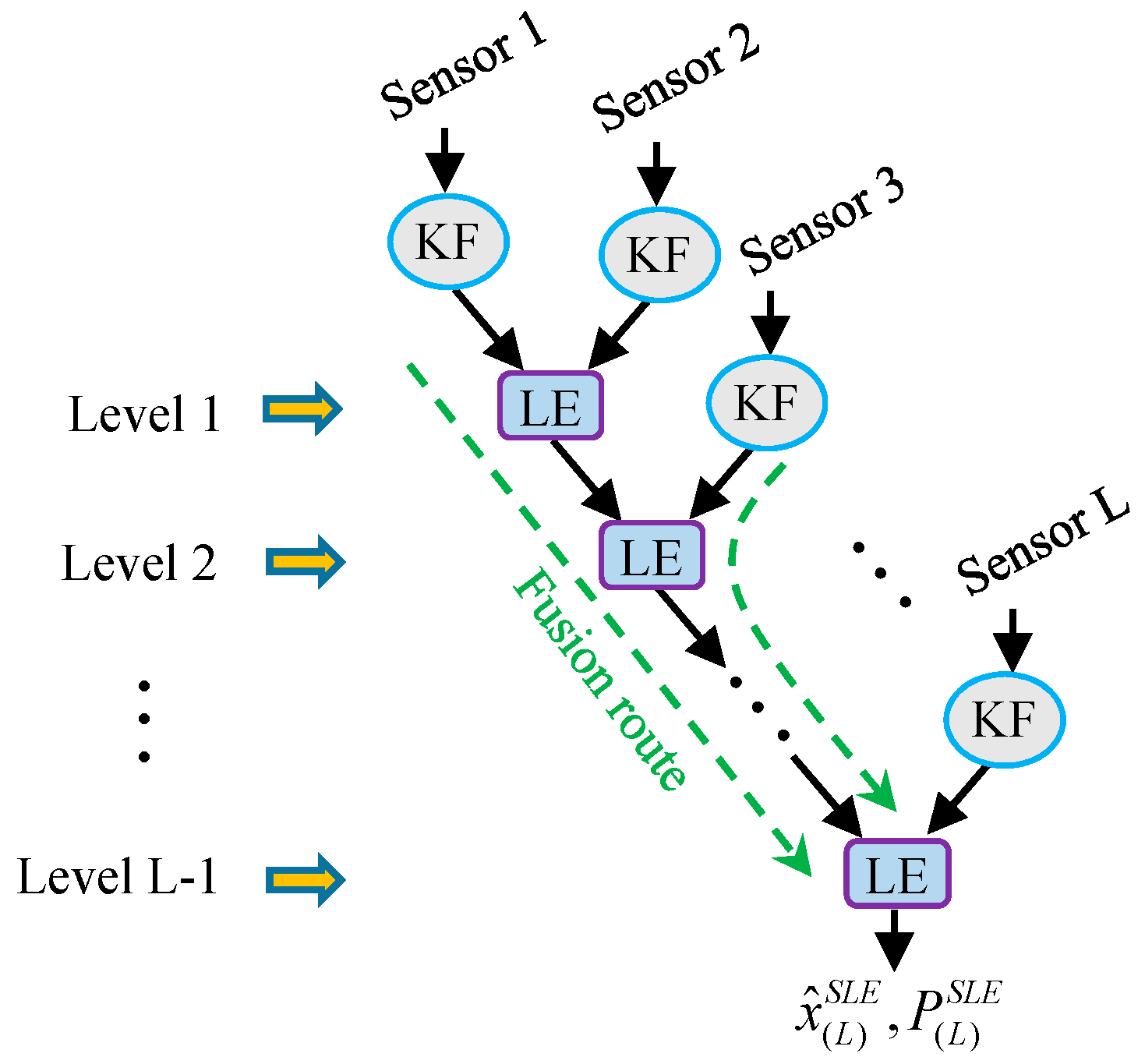
4.1. Multisensor Largest Ellipsoid Fuser with Sequential Structure
4.2. Multisensor Largest Ellipsoid Fusers with Parallel Structures
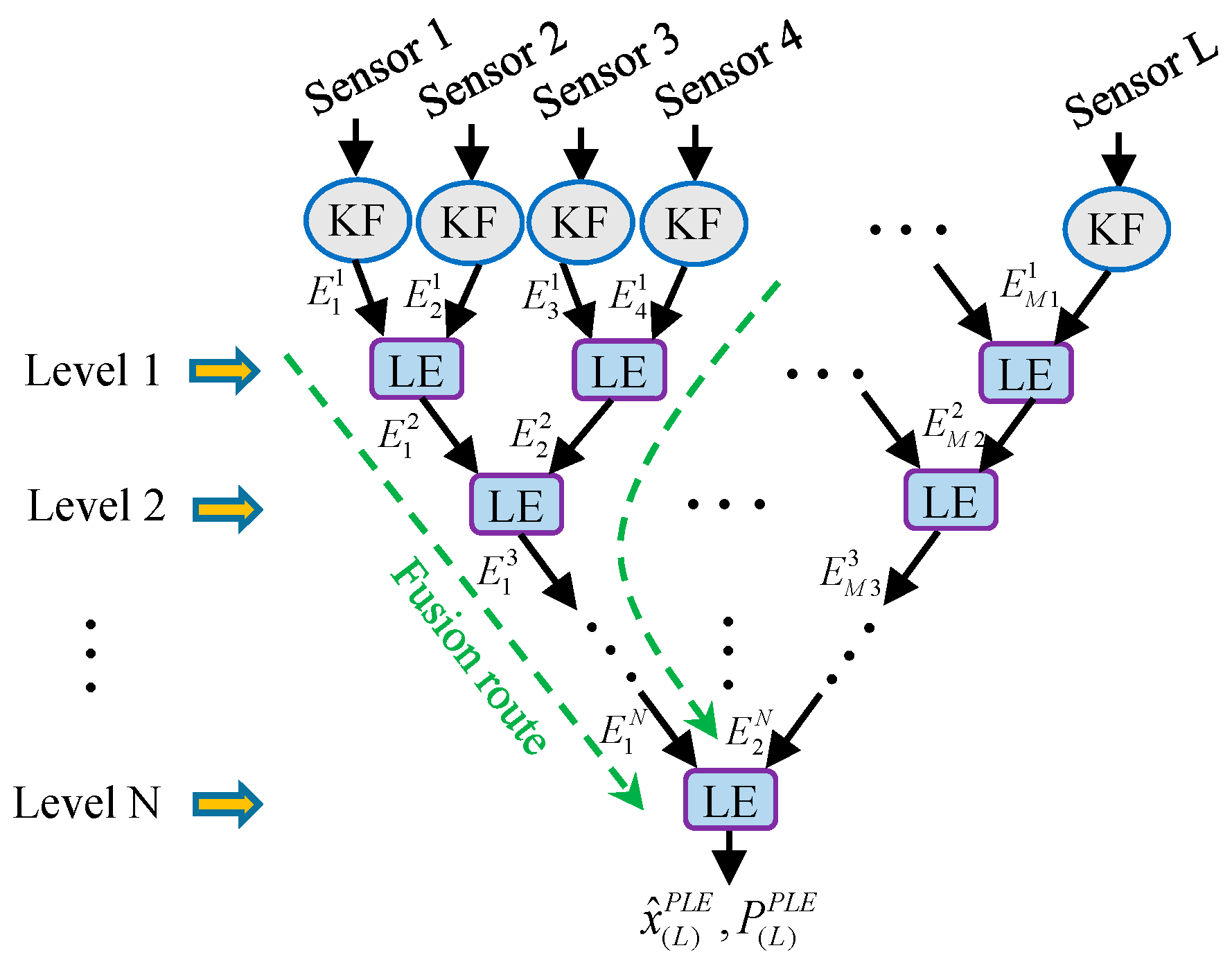
- Step 1: In the first fusion level, all of the local estimates received from local steady-state Kalman filters are fused in pairs using the LE algorithm. When the number of local estimates is even, we can get new fused estimates; and we can obtain new fused estimates including an unsettled local estimate when the number of local estimates is odd. Then, the new fused estimates are passed to the next fusion level.
- Step 2: As Step 1, all the estimates received from the upper fusion level are fused in pairs using the LE algorithm, and the obtained new fused estimates are passed to the next fusion level.
- Step N: There are only two estimates received from the upper fusion level in the fusion level and the fusion result of them through the LE algorithm is defined as the PLE fuser estimate .
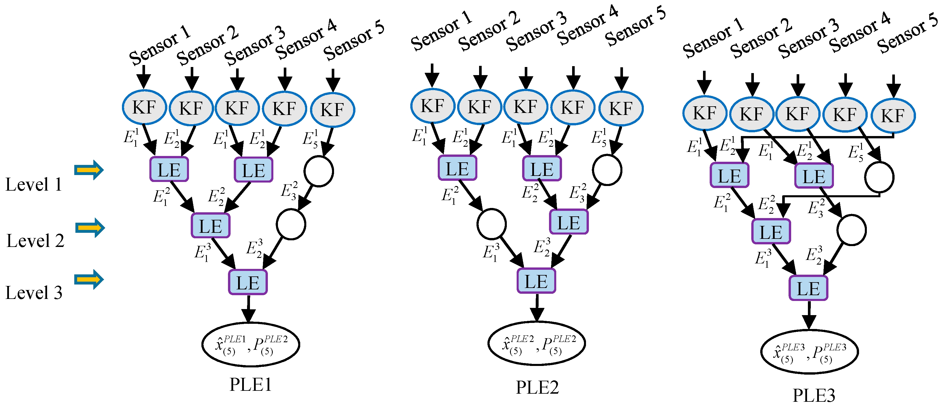
- Method 1:
- In the th fusion level, the received estimates are paired from to . If there is an unsettled received estimate in the th fusion level, it must be .
- Method 2:
- The fusion levels of this type of PLE fuser alternately pair their received estimates from to or from to . For instance, the local estimates are paired from to in the fusion level 1, the received estimates in the fusion level 2 are paired from to , and the received estimates in the fusion level 3 are paired from to , etc. If there is an unsettled received estimate in the th fusion level, it must be or .
- Method 3:
- In the th fusion level, the received estimates and are grouped into a pair with their fused estimate treated as in the next fusion level, and the remaining received estimates are paired from to . If there is an unsettled received estimate in the th fusion level, it must be .
4.3. Properties of Multisensor Largest Ellipsoid Fusers
5. Simulations and Analysis
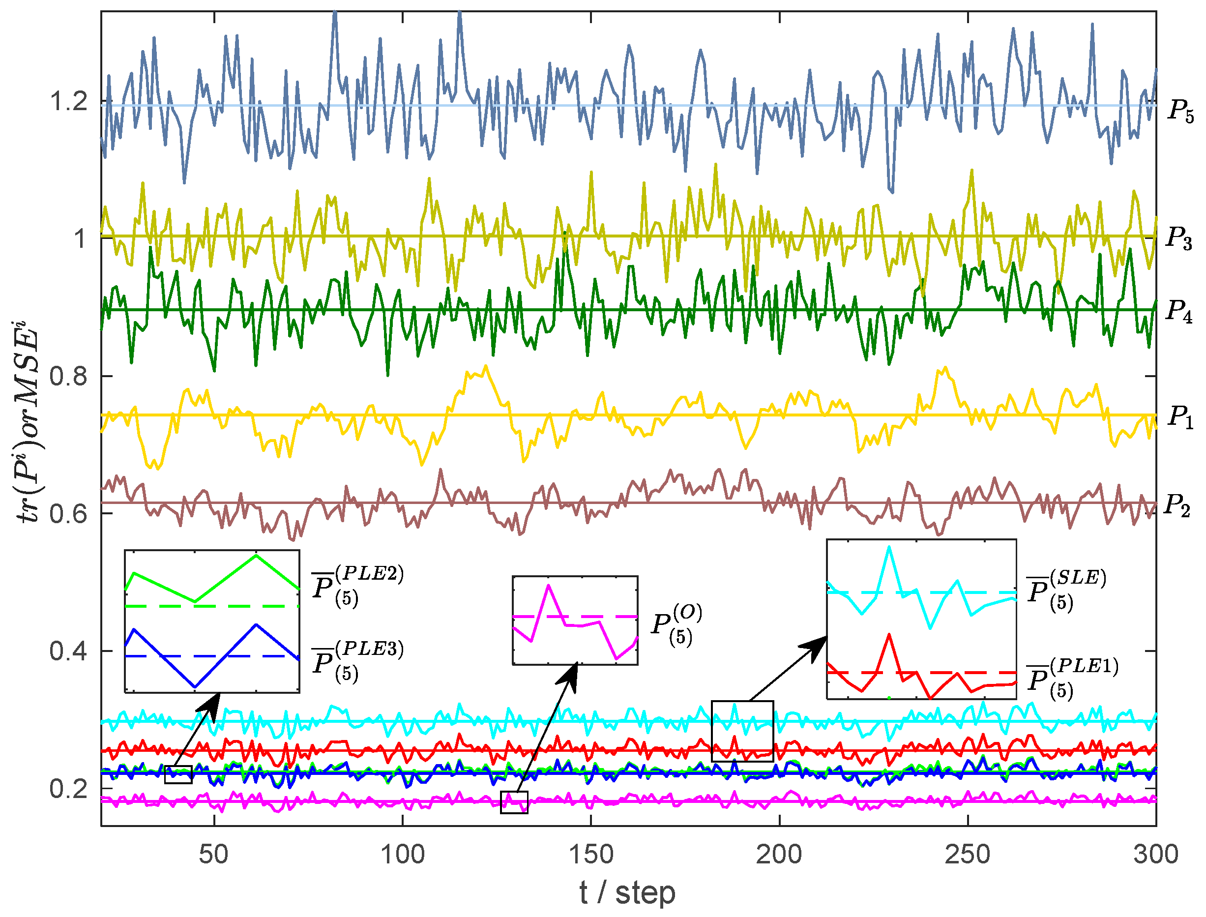
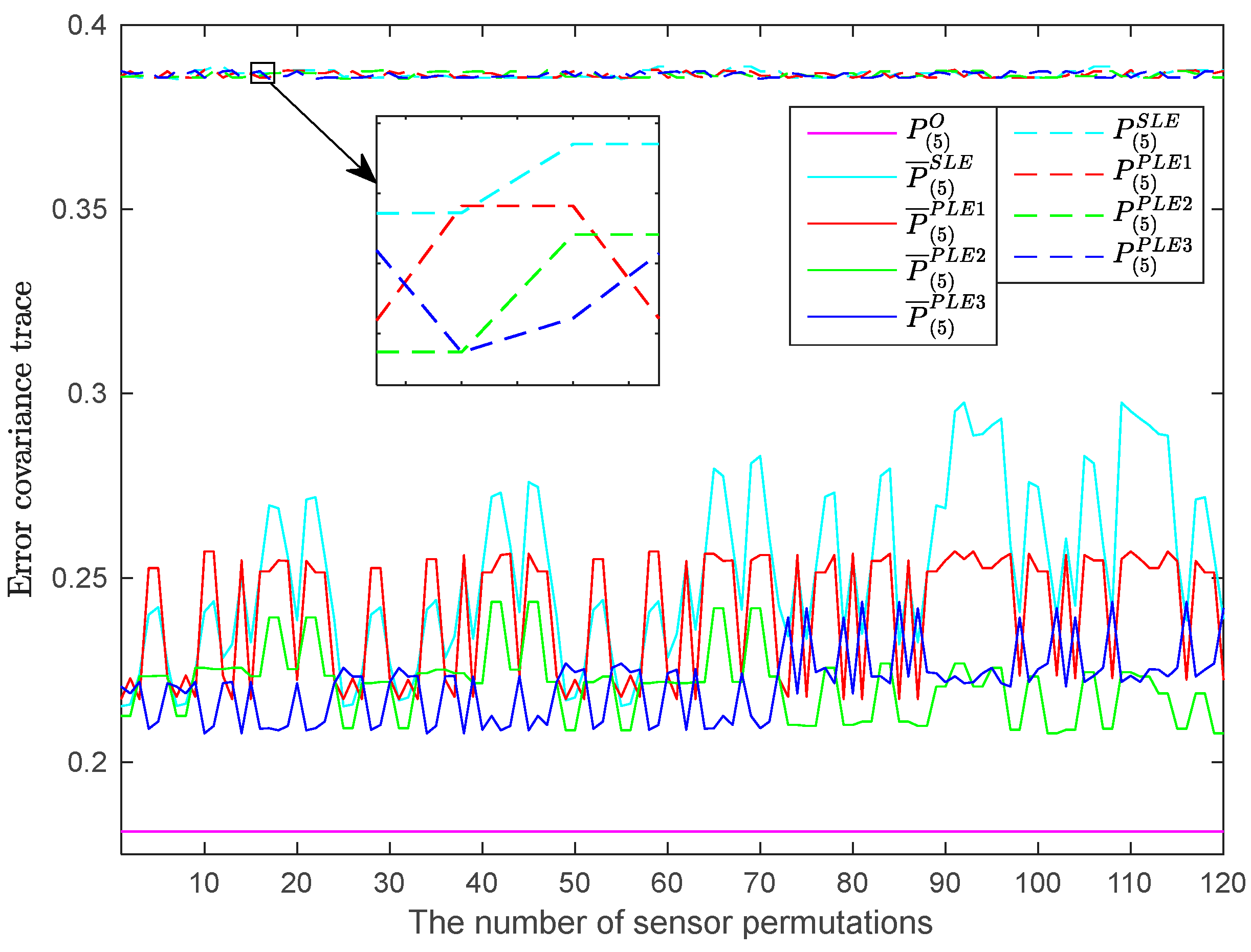
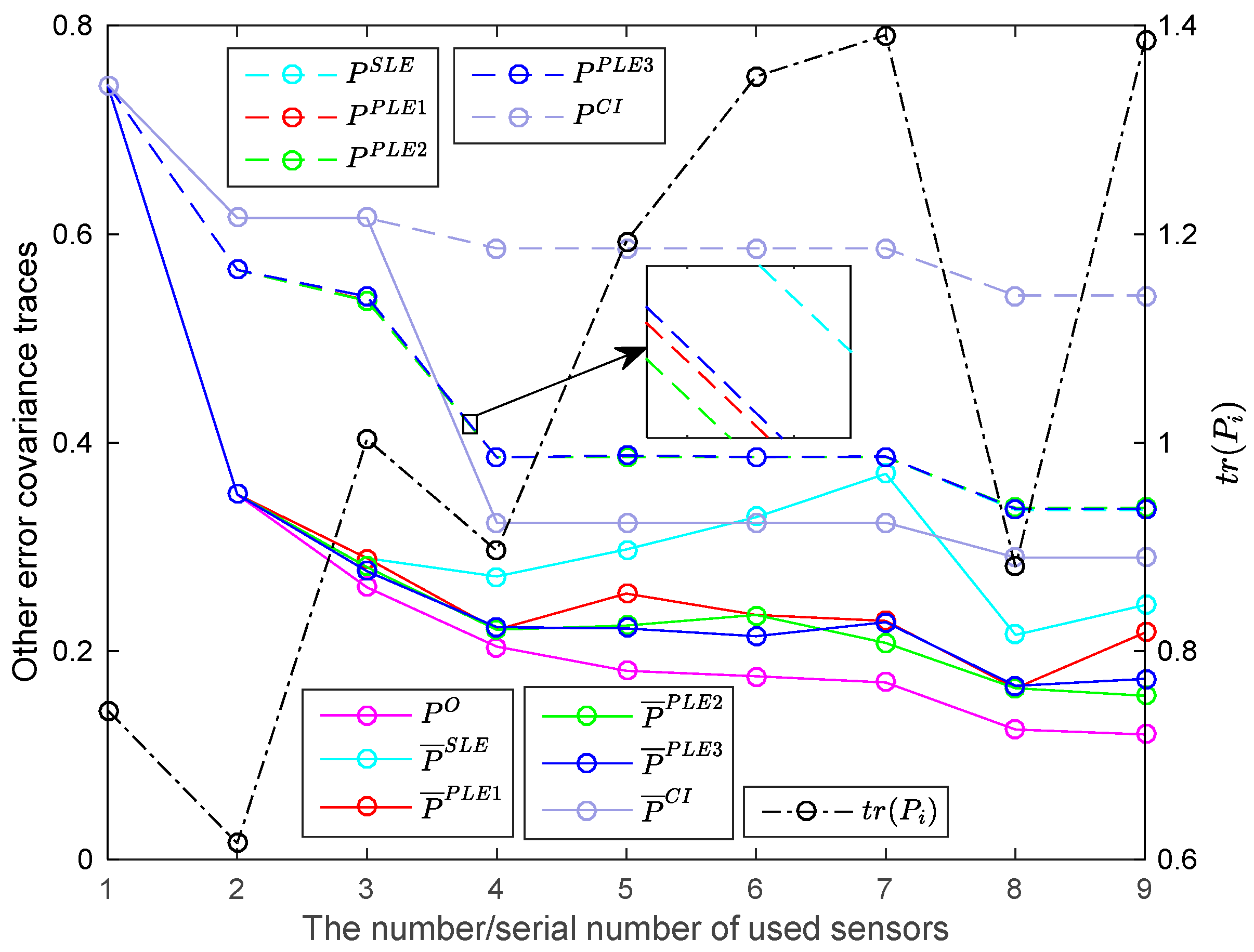
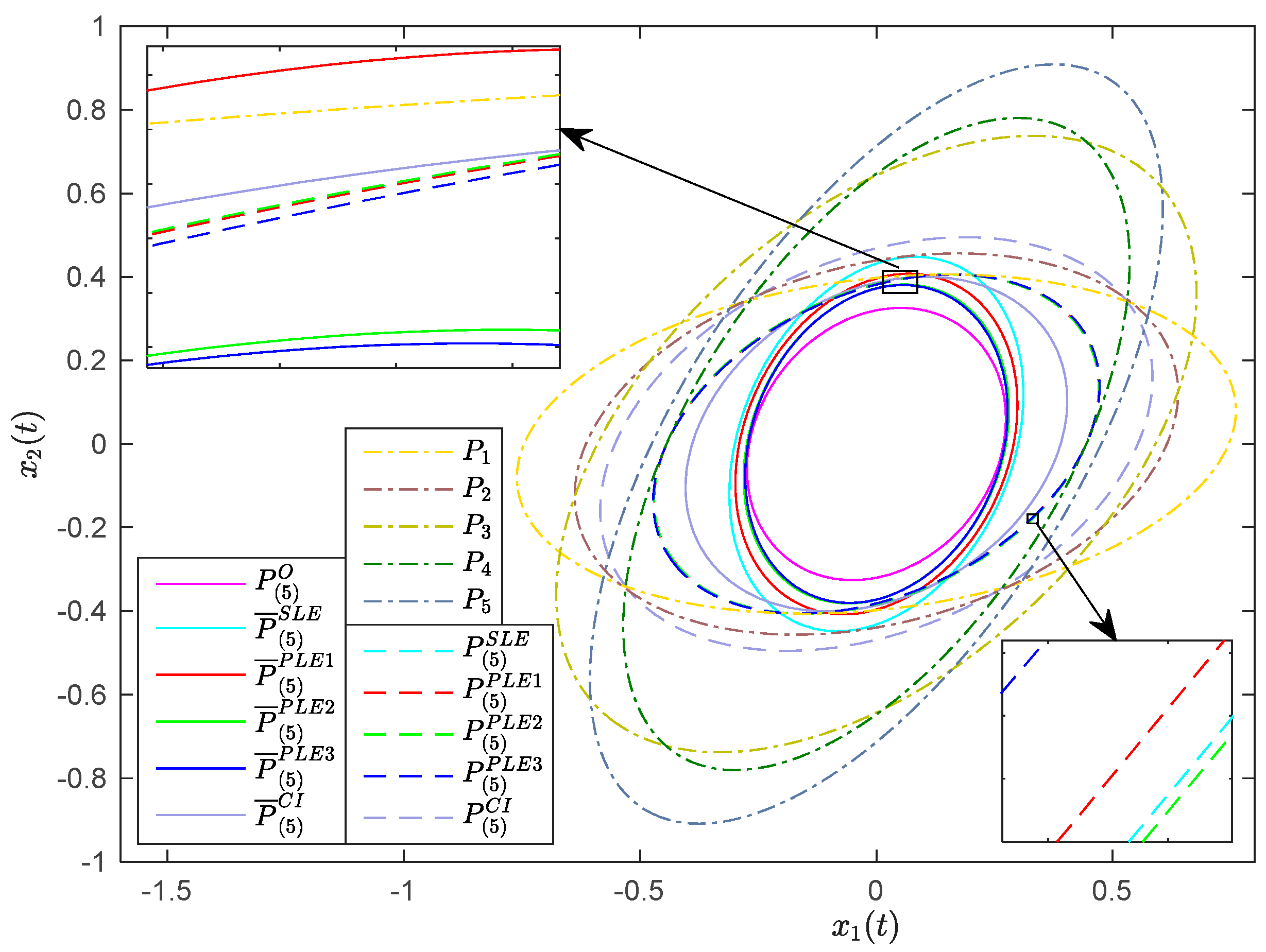
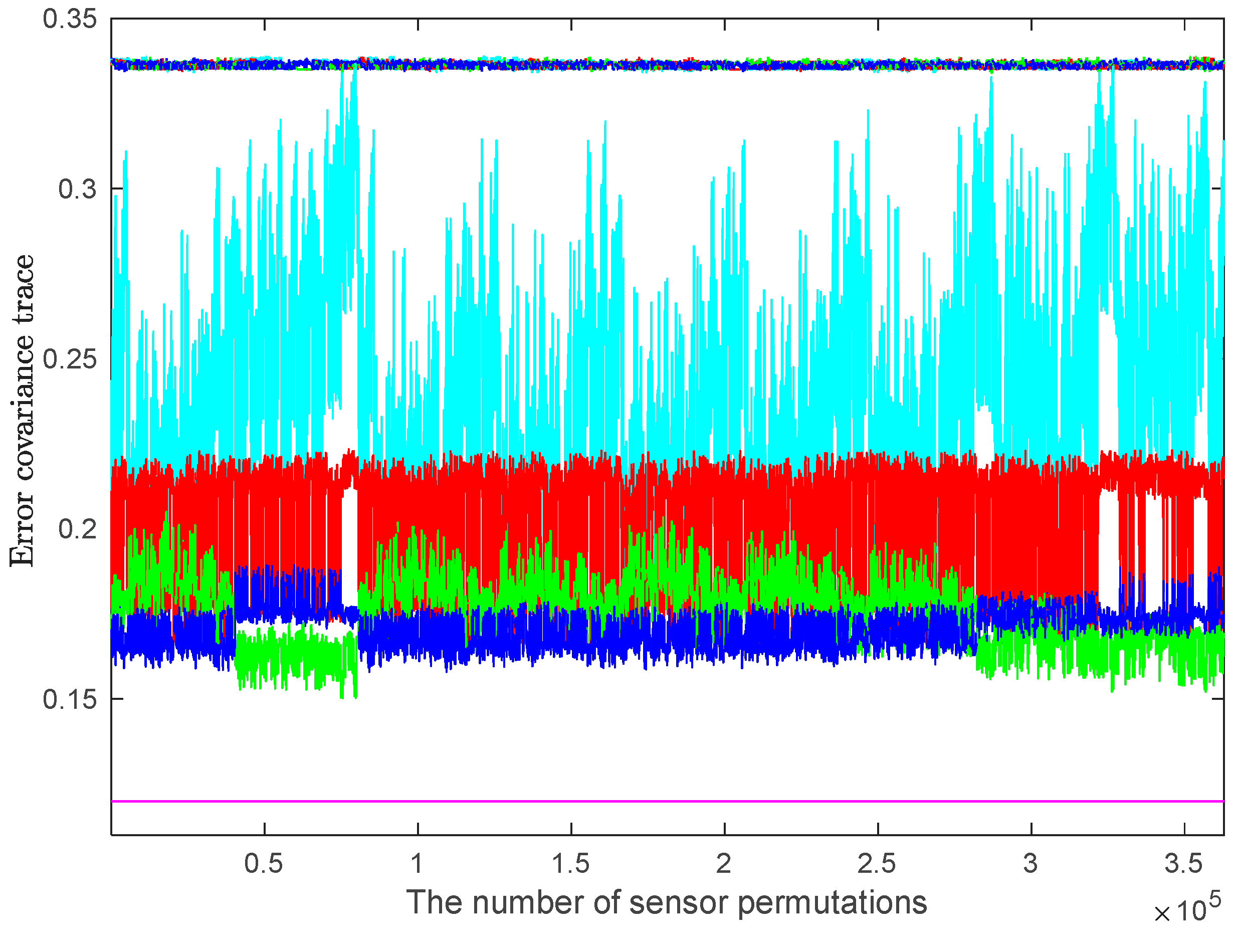
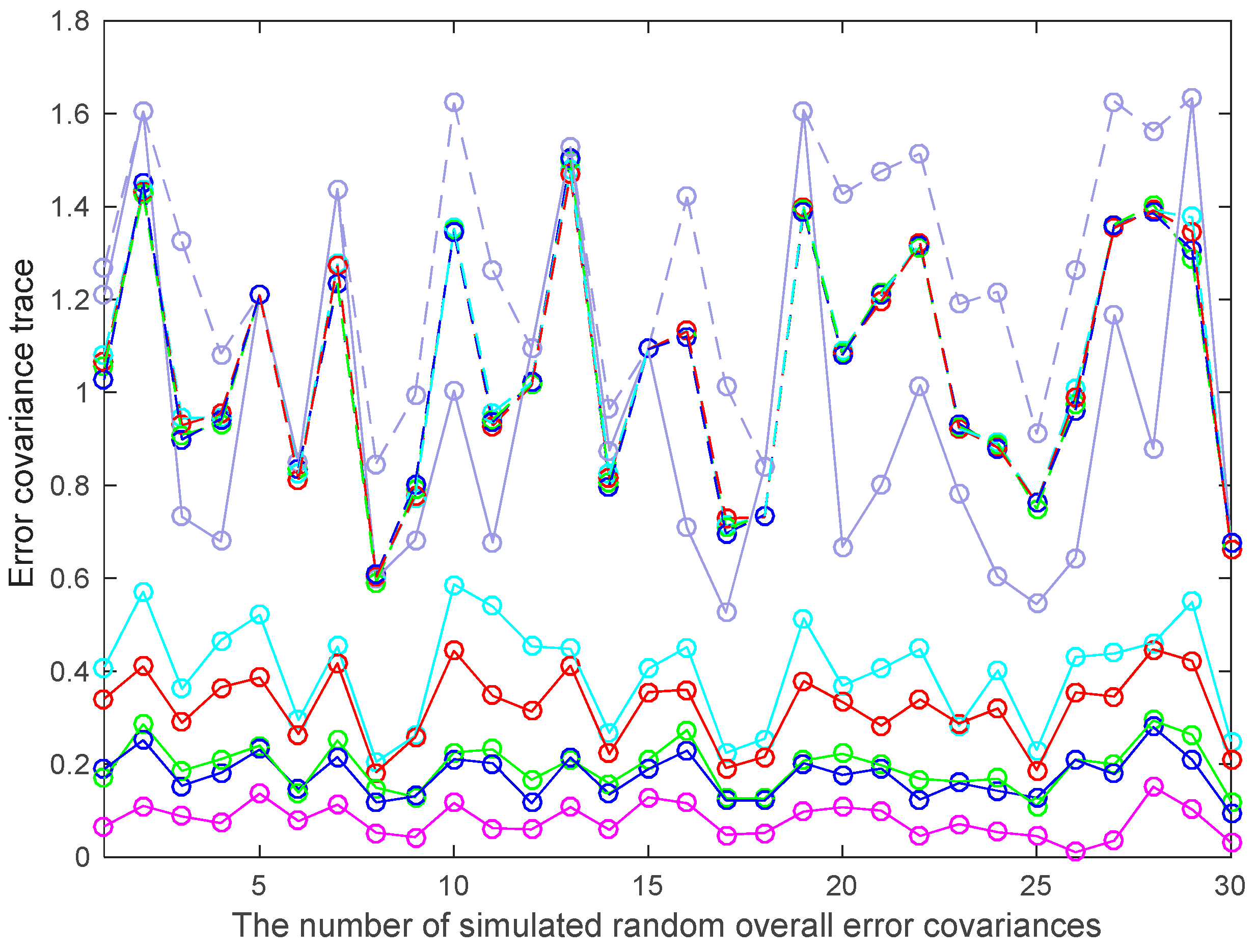
5.1. Simulations
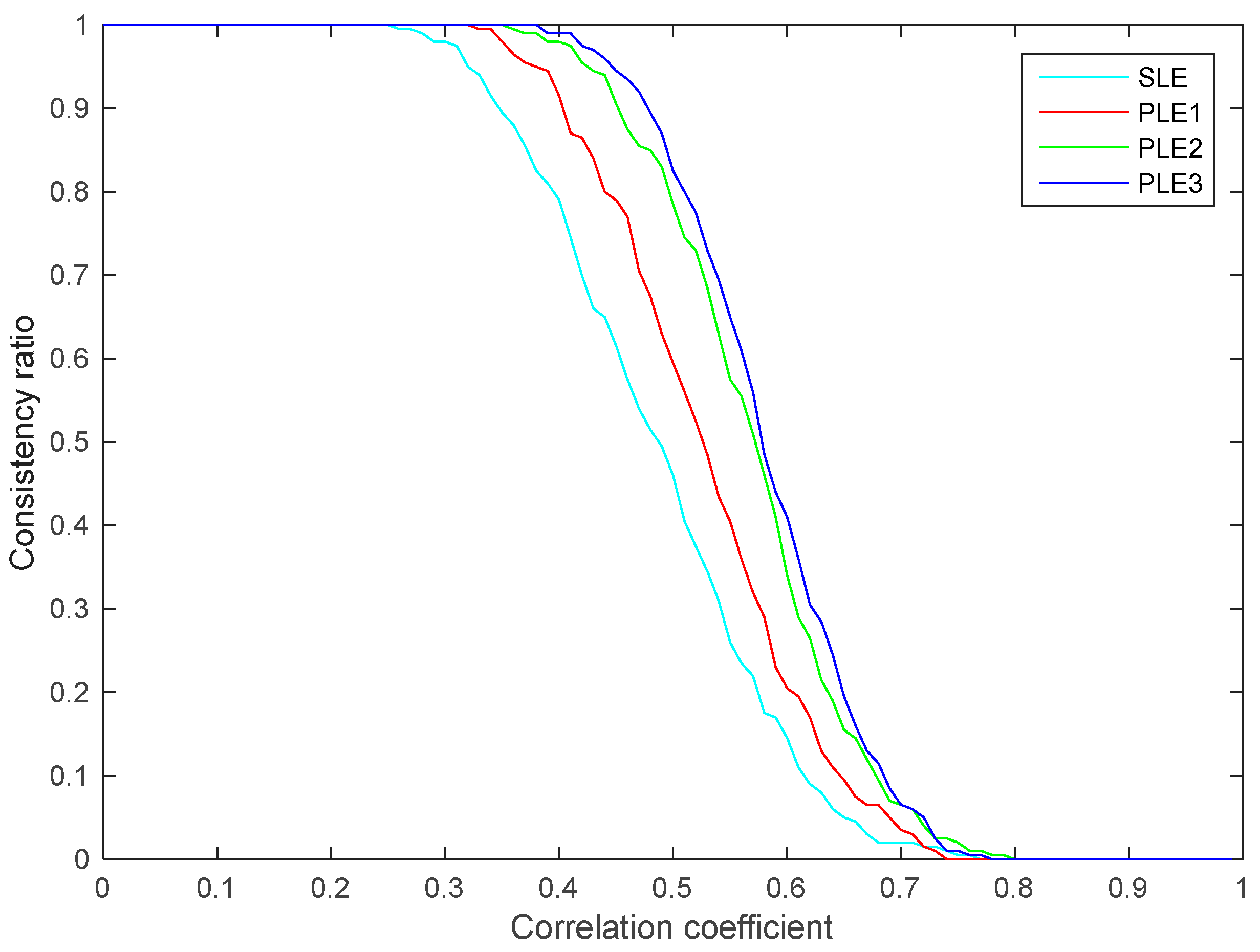
5.2. Analysis
6. Conclusions
Acknowledgments
Author Contributions
Conflicts of Interest
References
- Bar-Shalom, Y.; Campo, L. The effect of the common process noise on the two-sensor fused-track covariance. IEEE Trans. Aerosp. Electron. Syst. 1986, 22, 803–805. [Google Scholar] [CrossRef]
- Kim, K.H. Development of Track to Track Fusion Algorithms. In Proceedings of the American Control Conference, Baltimore, MD, USA, 29 June–1 July 1994; pp. 1037–1041. [Google Scholar]
- Sun, S.L.; Deng, Z.L. Multi-sensor optimal information fusion kalman filter. Automatica 2004, 40, 1017–1023. [Google Scholar] [CrossRef]
- Lewis, F.L. Optimal Estimation: With an Introduction to Stochastic Control Theory; John Wiley & Sons: New York, NY, USA, 1986. [Google Scholar]
- Sijs, J.; Lazar, M. State fusion with unknown correlation: Ellipsoidal intersection. Automatica 2012, 48, 1874–1878. [Google Scholar] [CrossRef]
- Benaskeur, A.R. Consistent Fusion of Correlated Data Sources. In Proceedings of the Annual Conference of the Industrial Electronics Society, Sevilla, Spain, 5–8 November 2002; pp. 2652–2656. [Google Scholar]
- Julier, S.J.; Uhlmann, J.K. A Non-Divergent Estimation Algorithm in the Presence of Unknown Correlations. In Proceedings of the American Control Conference, Alberqueque, NM, USA, 4–6 June 1997; pp. 2369–2373. [Google Scholar]
- Zhou, Y.; Li, J. Data Fusion of Unknown Correlations Using Internal Ellipsoidal Approximation. In Proceedings of the International Federation of Automatic Control, Seoul, Korea, 6–11 July 2008; pp. 2856–2860. [Google Scholar]
- Niehsen, W. Information Fusion Based on Fast Covariance Intersection Filtering. In Proceedings of the International Conference on Information Fusion, Annapolis, MD, USA, 8–11 July 2002; pp. 901–904. [Google Scholar]
- Khaleghi, B.; Khamis, A.; Karray, F.O.; Razavi, S.N. Multisensor data fusion: A review of the state-of-the-art. Inf. Fusion 2013, 14, 28–44. [Google Scholar] [CrossRef]
- Zhu, H.; Zhai, Q.; Yu, M.; Han, C. Estimation fusion algorithms in the presence of partially known cross-correlation of local estimation errors. Inf. Fusion 2014, 18, 187–196. [Google Scholar] [CrossRef]
- Julier, S.J.; Uhlmann, J.K. General Decentralized Data Fusion with Covariance Intersection (CI). In Handbook of Multisensor Data Fusion; Llinas, J., David, L.H., Eds.; CRC Press: Boca Raton, FL, USA, 2001; pp. 12.1–12.25. [Google Scholar]
- Wang, Y.; Li, X.R. Distributed estimation fusion with unavailable cross-correlation. IEEE Trans. Aerosp. Electron. Syst. 2012, 48, 259–278. [Google Scholar] [CrossRef]
- Franken, D.; Hupper, A. Improved Fast Covariance Intersection for Distributed Data Fusion. In Proceedings of the International Conference on Information Fusion, Philadelphia, PA, USA, 25–28 July 2005; pp. 154–160. [Google Scholar]
- Uhlmann, J.K. Covariance consistency methods for fault-tolerant distributed data fusion. Inf. Fusion 2003, 4, 201–215. [Google Scholar] [CrossRef]
- Wang, Y.; Li, X.R. Distributed estimation fusion under unknown cross-correlation: An analytic center approach. In Proceedings of the International Conference on Information Fusion, Edinburgh, UK, 26–29 July 2010; pp. 1–8. [Google Scholar]
- Farrell, W.J.; Ganesh, C. Generalized Chernoff Fusion Approximation for Practical Distributed Data Fusion. In Proceedings of the International Conference on Information Fusion, Seattle, WA, USA, 6–9 July 2009; pp. 555–562. [Google Scholar]
- Deng, Z.; Zhang, P.; Qi, W.; Liu, J.; Gao, Y. Sequential covariance intersection fusion kalman filter. Inf. Sci. 2012, 189, 293–309. [Google Scholar] [CrossRef]
- Wang, J.; Gao, Y.; Ran, C.; Huo, Y. State Estimation with Two-Level Fusion Structure. In Proceedings of the International Conference on Estimation, Detection and Information Fusion, Harbin, China, 10–11 January 2015; pp. 105–109. [Google Scholar]
- Nargess, S.N.; Poshtan, J.; Wagner, A.; Nordheimer, E.; Badreddin, E. Cascaded kalman and particle filters for photogrammetry based gyroscope drift and robot attitude estimation. ISA Trans. 2014, 53, 524–532. [Google Scholar]
- Bernstein, D.S. Matrix Mathematics: Theory, Facts, and Formulas, 2nd ed.; Princeton University Press: Princeton, NJ, USA, 2009. [Google Scholar]
- Deng, Z.; Zhang, P.; Qi, W.; Yuan, G.; Liu, J. The accuracy comparison of multisensor covariance intersection fuser and three weighting fusers. Inf. Fusion 2013, 14, 177–185. [Google Scholar] [CrossRef]
- Chen, L.; Arambel, P.O.; Mehra, R.K. Estimation under unknown correlation: Covariance intersection revisited. IEEE Trans. Autom. Control. 2002, 47, 1879–1882. [Google Scholar] [CrossRef]
- Carlson, N.A. Federated square root filter for decentralized parallel processors. IEEE Trans. Aerosp. Electron. Syst. 1990, 26, 517–525. [Google Scholar] [CrossRef]
- Lennart, L. System Identification, Theory for the User, 2nd ed.; Prentice Hall: Upper Saddle River, NJ, USA, 1999. [Google Scholar]


| 0.7433 | 0.6155 | 1.0032 | 0.8962 | 1.1932 | 0.1812 | 0.3233 | 0.5863 |
| 0.2976 | 0.3861 | 0.2550 | 0.3860 | 0.2244 | 0.3861 | 0.2217 | 0.3876 |
| 1.3512 | 1.3910 | 0.8807 | 1.3865 |
© 2017 by the authors. Licensee MDPI, Basel, Switzerland. This article is an open access article distributed under the terms and conditions of the Creative Commons Attribution (CC BY) license (http://creativecommons.org/licenses/by/4.0/).
Share and Cite
Liu, B.; Zhan, X.; Zhu, Z.H. Multisensor Parallel Largest Ellipsoid Distributed Data Fusion with Unknown Cross-Covariances. Sensors 2017, 17, 1526. https://doi.org/10.3390/s17071526
Liu B, Zhan X, Zhu ZH. Multisensor Parallel Largest Ellipsoid Distributed Data Fusion with Unknown Cross-Covariances. Sensors. 2017; 17(7):1526. https://doi.org/10.3390/s17071526
Chicago/Turabian StyleLiu, Baoyu, Xingqun Zhan, and Zheng H. Zhu. 2017. "Multisensor Parallel Largest Ellipsoid Distributed Data Fusion with Unknown Cross-Covariances" Sensors 17, no. 7: 1526. https://doi.org/10.3390/s17071526
APA StyleLiu, B., Zhan, X., & Zhu, Z. H. (2017). Multisensor Parallel Largest Ellipsoid Distributed Data Fusion with Unknown Cross-Covariances. Sensors, 17(7), 1526. https://doi.org/10.3390/s17071526