
The Use of IMMUs in a Water Environment: Instrument Validation and Application of 3D Multi-Body Kinematic Analysis in Medicine and Sport

 ,
,  ,
,  , and
, and 
Abstract
:1. Introduction
2. Materials and Methods
2.1. Instrument Validation
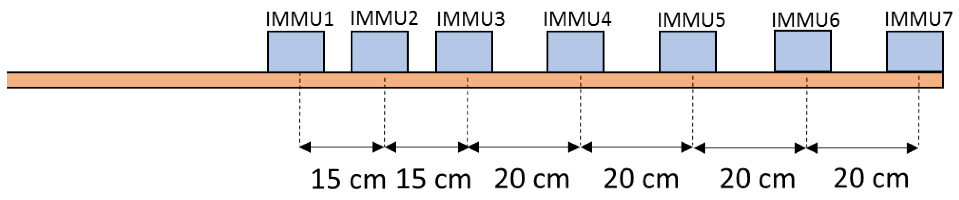
2.1.1. Sensors
2.1.2. Orientation Algorithm
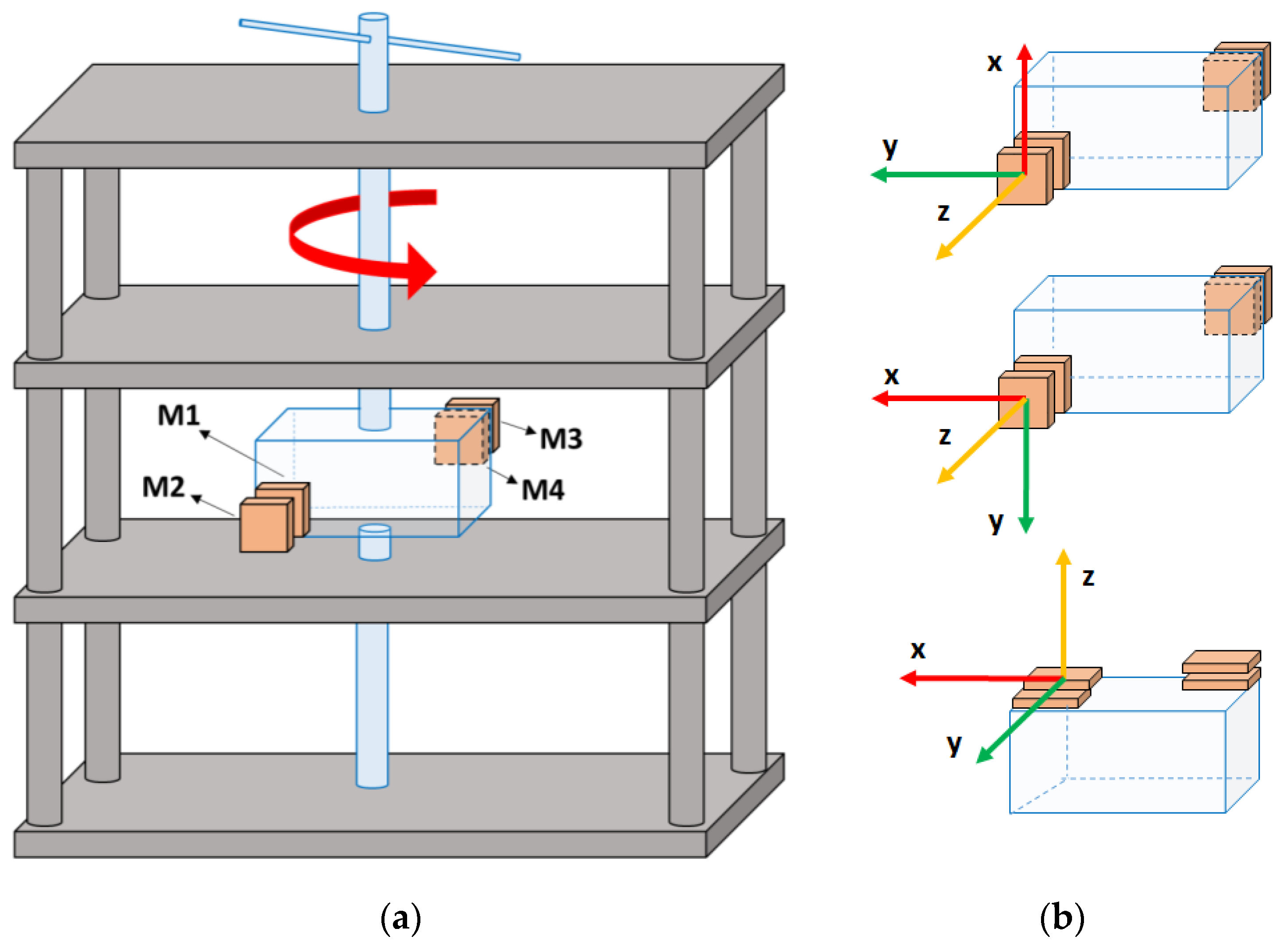
2.1.3. Magnetic Field Mapping
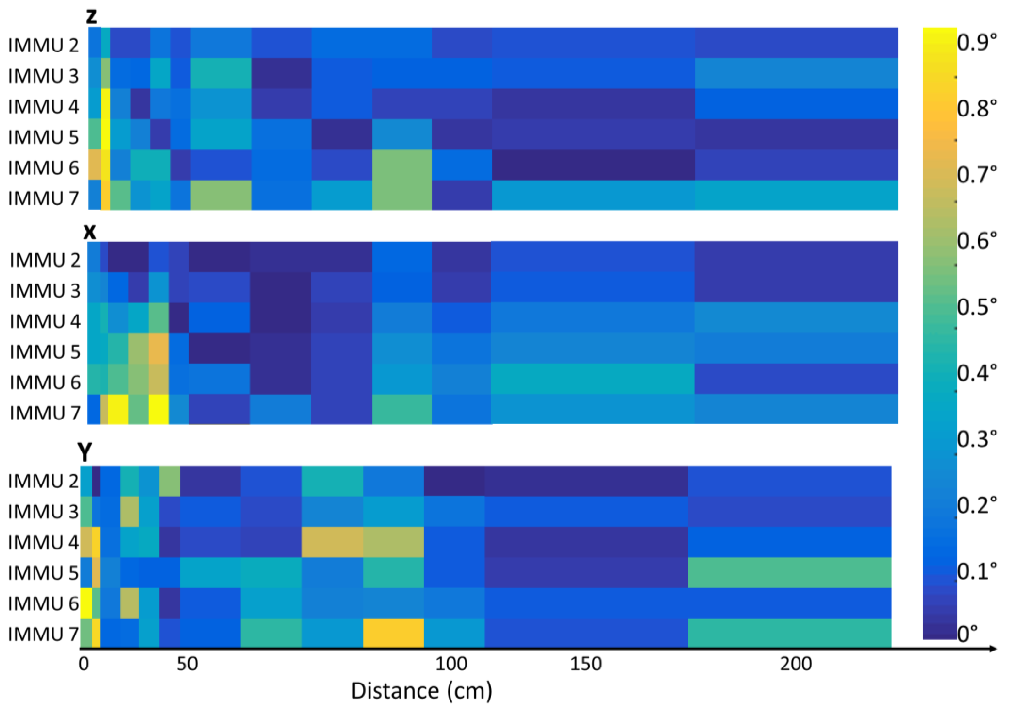
2.1.4. Dynamic Orientation Accuracy
2.2. Clinical and Sports Applications
2.2.1. Clinical Application: Gait Analysis
- (i)
- The investigation of healthy individuals’ kinematic variables during walking UW using IMMUs, and the definition of normative bands for healthy individuals
- (ii)
- The investigation and comparison of the healthy elderly kinematic variables with those found in younger adults
- (iii)
- The investigation and comparison of the kinematic variables of an anterior cruciate ligament (ACL) injured patient with those found in younger adults.
Lower Body Biomechanical Model
Set-Up
Participants
Motor Task
Data Analysis
2.2.2. Sport Applications: Swimming Analysis
- (i)
- Temporal phases detection
- (ii)
- Upper limb joint kinematic analysis
Upper Body Biomechanical Model
Set-Up
Participants and Motor Task
Data Analysis
3. Results
3.1. Instrument Validation
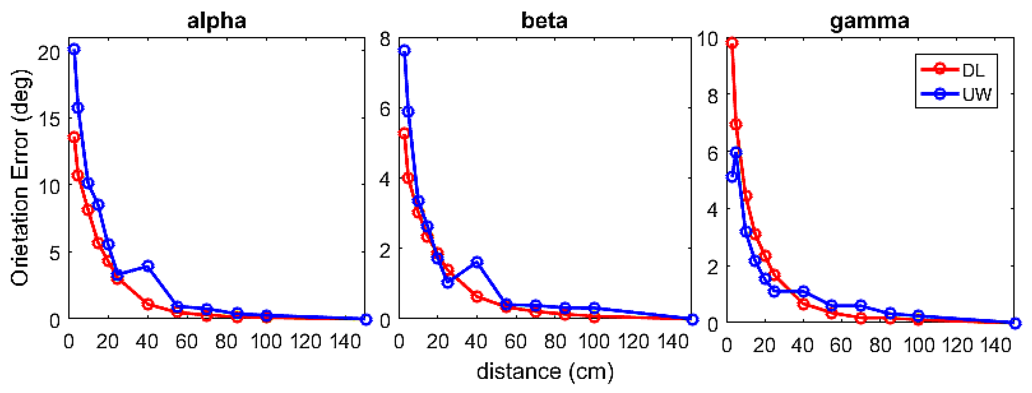
3.1.1. Magnetic Field Mapping
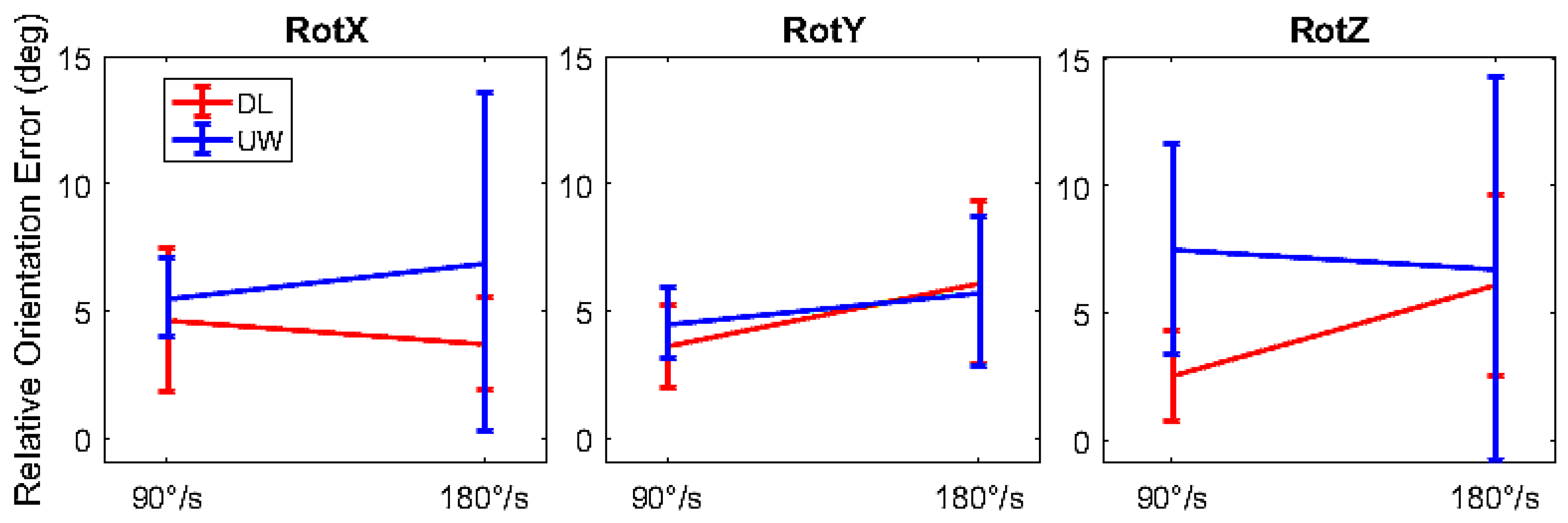
3.1.2. Dynamic Orientation Accuracy
3.2. Clinical and Sport Applications
3.2.1. Clinical Application: Gait Analysis
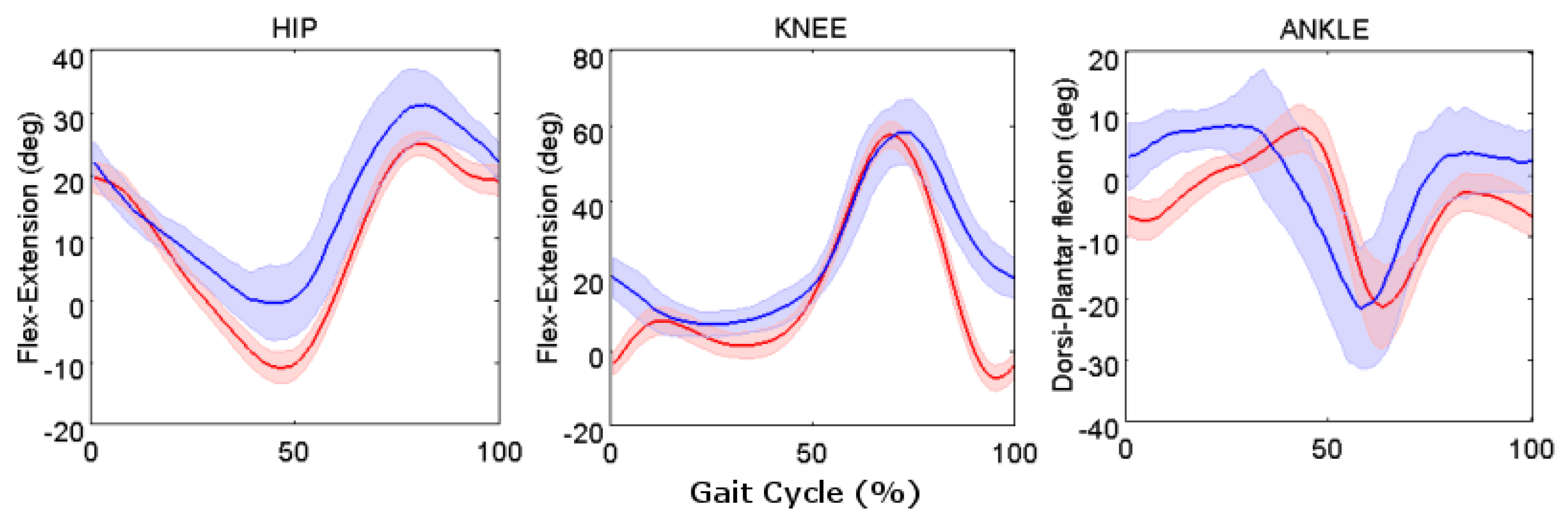
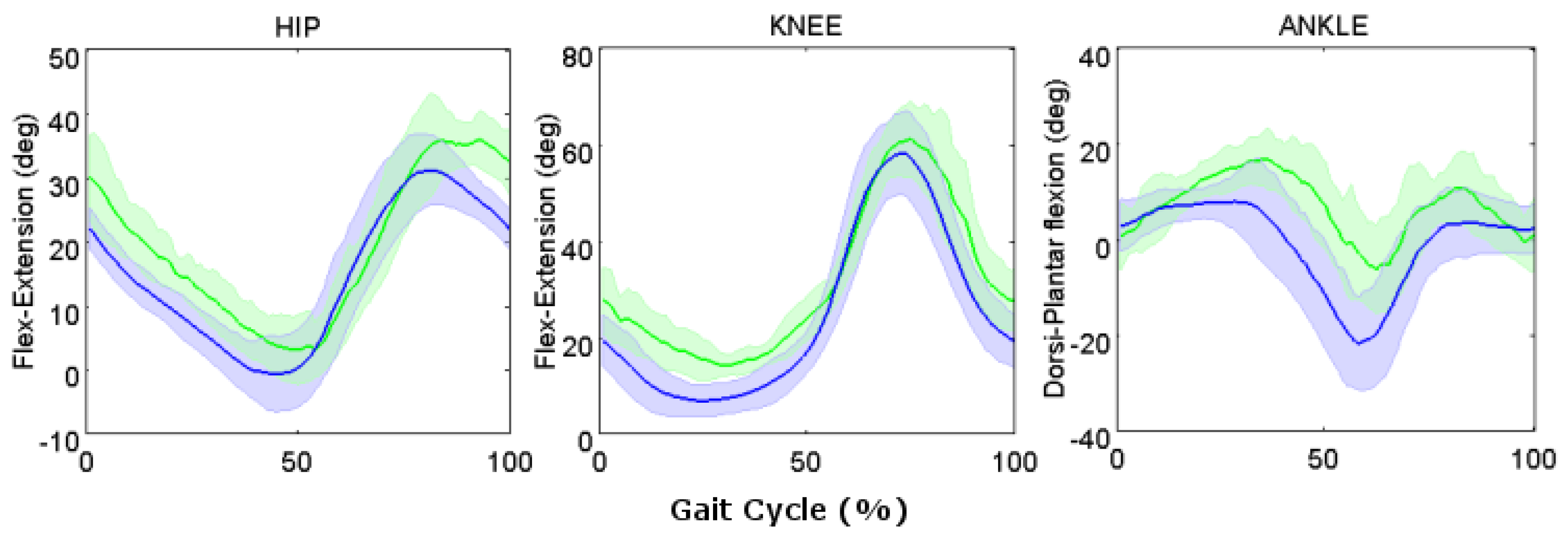
Healthy Young Adult Participants
Healthy Elderly Participants
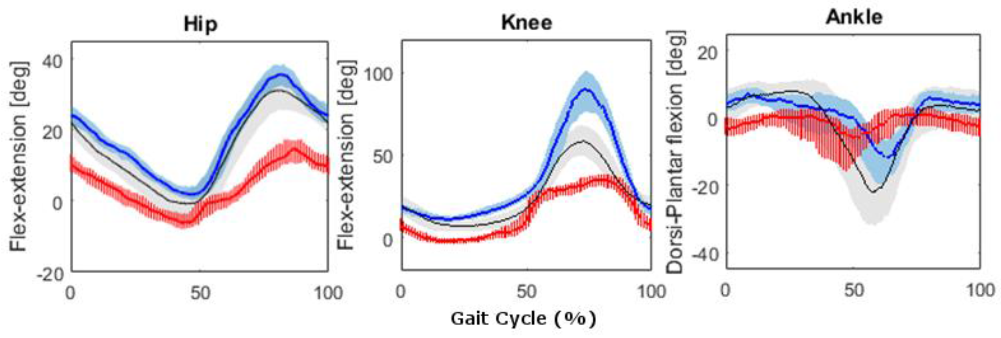
Pathological Participant
3.2.2. Sport Applications: Swimming Analysis
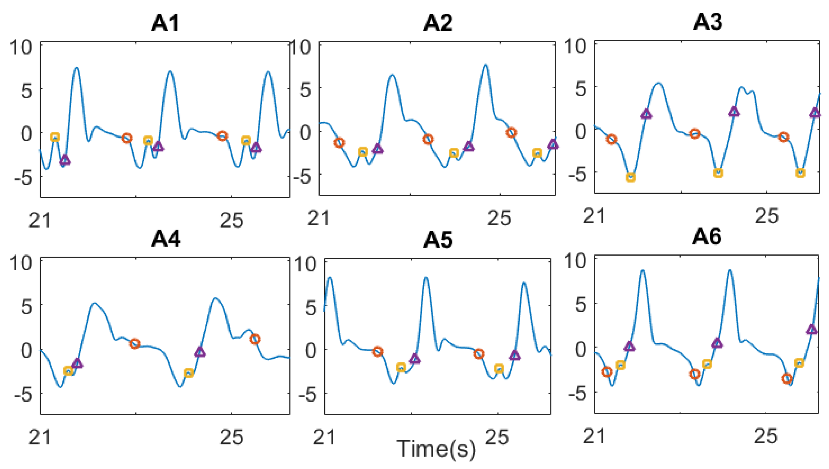
Temporal Phases Detection
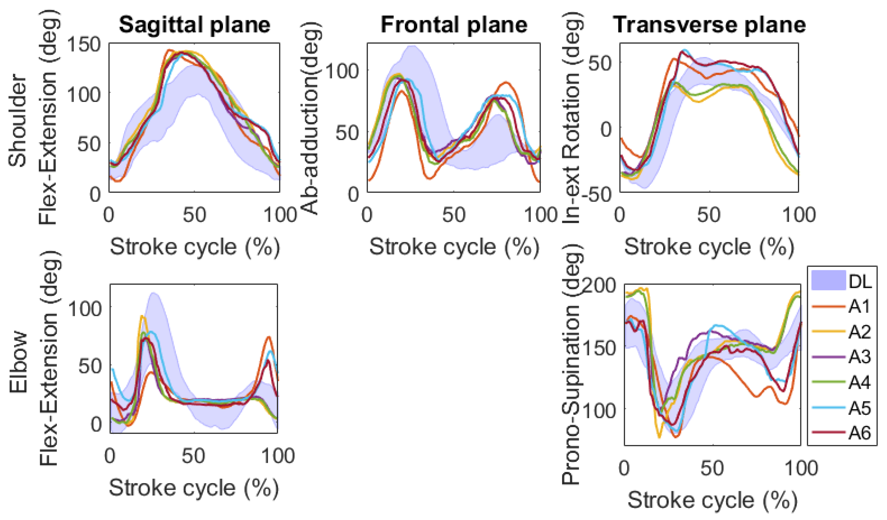
Joint Kinematic Analysis
4. Discussion
4.1. Instrument Validation
4.1.1. Magnetic Field Mapping
4.1.2. Dynamic Orientation Accuracy
4.2. Clinical and Sport Applications
4.2.1. Clinical Application: Gait Analysis
Healthy Young Adult Participants
Healthy Elderly Participants
Pathological Participants
4.2.2. Sport Application: Swimming Analysis
Temporal Phases Detection
Joint Kinematics Analysis
5. Conclusions
Acknowledgments
Author Contributions
Conflicts of Interest
References
- Callaway, A.J.; Cobb, J.E.; Jones, I. A comparison of video and accelerometer based approaches applied to performance monitoring in swimming. Int. J. Sports Sci. Coach. 2009, 4, 139–153. [Google Scholar] [CrossRef]
- Daukantas, S.; Marozas, V.; Lukosevicius, A. Inertial sensor for objective evaluation of swimmer performance. In Proceedings of the 11th International Biennial Baltic Electronics Conference, BEC 2008, Tallinn, Estonia, 6–8 October 2008; pp. 321–324. [Google Scholar]
- Muro-de-la-Herran, A.; Garcia-Zapirain, B.; Mendez-Zorrilla, A. Gait analysis methods: An overview of wearable and non-wearable systems, highlighting clinical applications. Sensors 2014, 14, 3362–3394. [Google Scholar] [CrossRef] [PubMed]
- Mooney, R.; Corley, G.; Godfrey, A.; Osborough, C.; Newell, J.; Quinlan, L.R.; ÓLaighin, G. Analysis of swimming performance: Perceptions and practices of US-based swimming coaches. J. Sports Sci. 2016, 34, 997–1005. [Google Scholar] [CrossRef] [PubMed]
- James, D.A.; Petrone, N. Sensors and Wearable Technologies in Sport: Technologies, Trends and Approaches for Implementation; Springer: Berlin, Germany, 2016. [Google Scholar]
- Silva, A.S.; Salazar, A.J.; Borges, C.M.; Correia, M.V. Wearable monitoring unit for swimming performance analysis. Proceedings of International Joint Conference on Biomedical Engineering Systems and Technologies BIOSTEC 2011, Rome, Italy, 26–29 January 2011; pp. 80–93. [Google Scholar]
- Ceseracciu, E.; Sawacha, Z.; Fantozzi, S.; Cortesi, M.; Gatta, G.; Corazza, S.; Cobelli, C. Markerless analysis of front crawl swimming. J. Biomech. 2011, 44, 2236–2242. [Google Scholar] [CrossRef] [PubMed]
- Cortesi, M.; Fantozzi, S.; Gatta, G. Effects of distance specialization on the backstroke swimming kinematics. J. Sports Sci. Med. 2012, 11, 526–532. [Google Scholar] [PubMed]
- McCabe, C.B.; Sanders, R.H. Kinematic differences between front crawl sprint and distance swimmers at a distance pace. J. Sports Sci. 2012, 30, 601–608. [Google Scholar] [CrossRef] [PubMed]
- Smith, D.J.; Norris, S.R.; Hogg, J.M. Performance evaluation of swimmers. Sports Med. 2002, 32, 539–554. [Google Scholar] [CrossRef] [PubMed]
- Tamburella, F.; Scivoletto, G.; Cosentino, E.; Molinari, M. Walking in water and on land after an incomplete spinal cord injury. Am. J. Phys. Med. Rehabil. 2013, 92, e4–e15. [Google Scholar] [CrossRef] [PubMed]
- Ceccon, S.; Ceseracciu, E.; Sawacha, Z.; Gatta, G.; Cortesi, M.; Cobelli, C.; Fantozzi, S. Motion analysis of front crawl swimming applying cast technique by means of automatic tracking. J. Sports Sci. 2013, 31, 276–287. [Google Scholar] [CrossRef] [PubMed]
- Gourgoulis, V.; Aggeloussis, N.; Kasimatis, P.; Vezos, N.; Boli, A.; Mavromatis, G. Reconstruction accuracy in underwater three-dimensional kinematic analysis. J. Sci. Med. Sport 2008, 11, 90–95. [Google Scholar] [CrossRef] [PubMed]
- Magalhaes, F.A.; Sawacha, Z.; Di Michele, R.; Cortesi, M.; Gatta, G.; Fantozzi, S. Effectiveness of an automatic tracking software in underwater motion analysis. J. Sports Sci. Med. 2013, 12, 660–667. [Google Scholar] [PubMed]
- Wilson, D.J.; Smith, B.K.; Gibson, J.K.; Choe, B.K. Accuracy of digitization using automated and manual methods. Phys. Ther. 1999, 79, 558–566. [Google Scholar] [PubMed]
- Newell, K.; Walter, C.B. Kinematic and kinetic parameters as information feedback in motor skill acquisition. J. Hum. Mov. Stud. 1981, 7, 235–254. [Google Scholar]
- James, D.A. The application of inertial sensors in elite sports monitoring. In The Engineering of Sport 6; Springer: Berlin, Germany, 2006; pp. 289–294. [Google Scholar]
- Madgwick, S.O.; Harrison, A.J.; Vaidyanathan, R. Estimation of imu and marg orientation using a gradient descent algorithm. In Proceedings of the 2011 IEEE International Conference on Rehabilitation Robotics, Zurich, Switzerland, 29 June–1 July 2011; pp. 1–7. [Google Scholar]
- Bonato, P. Advances in wearable technology and applications in physical medicine and rehabilitation. J. NeuroEng. Rehabil. 2005, 2. [Google Scholar] [CrossRef] [PubMed]
- Cuesta-Vargas, A.I.; Galán-Mercant, A.; Williams, J.M. The use of inertial sensors system for human motion analysis. Phys. Ther. Rev. 2010, 15, 462–473. [Google Scholar] [CrossRef] [PubMed]
- Fong, D.T.-P.; Chan, Y.-Y. The use of wearable inertial motion sensors in human lower limb biomechanics studies: A systematic review. Sensors 2010, 10, 11556–11565. [Google Scholar] [CrossRef] [PubMed]
- Mathie, M.J.; Coster, A.C.; Lovell, N.H.; Celler, B.G. Accelerometry: Providing an integrated, practical method for long-term, ambulatory monitoring of human movement. Physiol. Meas. 2004, 25, R1. [Google Scholar] [CrossRef] [PubMed]
- Cutti, A.G.; Ferrari, A.; Garofalo, P.; Raggi, M.; Cappello, A.; Ferrari, A. ‘Outwalk’: A protocol for clinical gait analysis based on inertial and magnetic sensors. Med. Biol. Eng. Comput. 2009, 48, 17. [Google Scholar] [CrossRef] [PubMed]
- Saber-Sheikh, K.; Bryant, E.C.; Glazzard, C.; Hamel, A.; Lee, R.Y. Feasibility of using inertial sensors to assess human movement. Man. Ther. 2010, 15, 122–125. [Google Scholar] [CrossRef] [PubMed]
- Tadano, S.; Takeda, R.; Miyagawa, H. Three dimensional gait analysis using wearable acceleration and gyro sensors based on quaternion calculations. Sensors 2013, 13, 9321–9343. [Google Scholar] [CrossRef] [PubMed]
- Weiss, A.; Herman, T.; Plotnik, M.; Brozgol, M.; Maidan, I.; Giladi, N.; Gurevich, T.; Hausdorff, J.M. Can an accelerometer enhance the utility of the timed up & go test when evaluating patients with parkinson’s disease? Med. Eng. Phys. 2010, 32, 119–125. [Google Scholar] [PubMed]
- Kaneda, K.; Mckean, M.; Ohgi, Y.; Burkett, B. Walking and running kinesiology in water: A review of the literature. J. Fit. Res. 2012, 1, 1–11. [Google Scholar]
- Severin, A.C.; Burkett, B.J.; McKean, M.R.; Sayers, M.G. Biomechanical aspects of aquatic therapy: A literature review on application and methodological challenges. J. Fit. Res. 2016, 5, 48–62. [Google Scholar]
- Marinho-Buzelli, A.R.; Rouhani, H.; Masani, K.; Verrier, M.C.; Popovic, M.R. The influence of the aquatic environment on the control of postural sway. Gait Posture 2017, 51, 70–76. [Google Scholar] [CrossRef] [PubMed]
- Ohgi, Y.; Yasumura, M.; Ichikawa, H.; Miyaji, C. Analysis of stroke technique using acceleration sensor ic in freestyle swimming. Eng. Sport 2000, 250, 503–511. [Google Scholar]
- Wright, B.V.; Stager, J.M. Quantifying competitive swim training using accelerometer-based activity monitors. Sports Eng. 2013, 16, 155–164. [Google Scholar] [CrossRef]
- Fantozzi, S.; Giovanardi, A.; Borra, D.; Gatta, G. Gait kinematic analysis in water using wearable inertial magnetic sensors. PLoS ONE 2015, 10, e0138105. [Google Scholar] [CrossRef] [PubMed]
- Fantozzi, S.; Giovanardi, A.; Magalhães, F.A.; Di Michele, R.; Cortesi, M.; Gatta, G. Assessment of three-dimensional joint kinematics of the upper limb during simulated swimming using wearable inertial-magnetic measurement units. J. Sports Sci. 2016, 34, 1073–1080. [Google Scholar] [CrossRef] [PubMed]
- Le Sage, T.; Bindel, A.; Conway, P.; Justham, L.; Slawson, S.; West, A. Embedded programming and real-time signal processing of swimming strokes. Sports Eng. 2011, 14, 1. [Google Scholar] [CrossRef]
- Brodie, M.; Walmsley, A.; Page, W. The static accuracy and calibration of inertial measurement units for 3D orientation. Comput. Methods Biomech. Biomed. Eng. 2008, 11, 641–648. [Google Scholar] [CrossRef] [PubMed]
- Cutti, A.G.; Giovanardi, A.; Rocchi, L.; Davalli, A. A simple test to assess the static and dynamic accuracy of an inertial sensors system for human movement analysis. Proceedings of 28th Annual International Conference of the IEEE Engineering in Medicine and Biology Society, EMBS ’06, New York, NY, USA, 30 August–3 September 2006; pp. 5912–5915. [Google Scholar]
- Godwin, A.; Agnew, M.; Stevenson, J. Accuracy of inertial motion sensors in static, quasistatic, and complex dynamic motion. J. Biomech. Eng. 2009, 131, 114501. [Google Scholar] [CrossRef] [PubMed]
- Picerno, P.; Cereatti, A.; Cappozzo, A. A spot check for assessing static orientation consistency of inertial and magnetic sensing units. Gait Posture 2011, 33, 373–378. [Google Scholar] [CrossRef] [PubMed]
- Barela, A.M.; Duarte, M. Biomechanical characteristics of elderly individuals walking on land and in water. J. Electromyogr. Kinesiol. 2008, 18, 446–454. [Google Scholar] [CrossRef] [PubMed]
- Lebel, K.; Boissy, P.; Hamel, M.; Duval, C. Inertial measures of motion for clinical biomechanics: Comparative assessment of accuracy under controlled conditions-effect of velocity. PLoS ONE 2013, 8, e79945. [Google Scholar] [CrossRef] [PubMed]
- Lebel, K.; Boissy, P.; Hamel, M.; Duval, C. Inertial measures of motion for clinical biomechanics: Comparative assessment of accuracy under controlled conditions—Changes in accuracy over time. PLoS ONE 2015, 10, e0118361. [Google Scholar] [CrossRef] [PubMed]
- Ricci, L.; Taffoni, F.; Formica, D. On the orientation error of imu: Investigating static and dynamic accuracy targeting human motion. PLoS ONE 2016, 11, e0161940. [Google Scholar] [CrossRef] [PubMed]
- Bachmann, E.R.; Xiaoping, Y.; Peterson, C.W. An investigation of the effects of magnetic variations on inertial/magnetic orientation sensors. In Proceedings of the 2004 IEEE International Conference on Robotics and Automation, ICRA ’04, New Orleans, LA, USA, 26 April–1 May 2004; Volume 1112, pp. 1115–1122. [Google Scholar]
- De Vries, W.; Veeger, H.; Baten, C.; Van Der Helm, F. Magnetic distortion in motion labs, implications for validating inertial magnetic sensors. Gait Posture 2009, 29, 535–541. [Google Scholar] [CrossRef] [PubMed]
- Becker, B.E. Aquatic therapy: Scientific foundations and clinical rehabilitation applications. PM R 2009, 1, 859–872. [Google Scholar] [CrossRef] [PubMed]
- Bates, A.; Consulting, A.E.T.; Hanson, N. Aquatic Exercise Therapy: A Comprehensive Approach to the Use of Aquatic Exercise in the Treatment of Orthopedic Injuries; Aquatic Exercise Therapy Consulting: Victoria, BC, Canada, 1992. [Google Scholar]
- Devereux, K.; Robertson, D.; Briffa, N.K. Effects of a water-based program on women 65 years and over: A randomised controlled trial. Aust. J. Physiother. 2005, 51, 102–108. [Google Scholar] [CrossRef]
- Suomi, R.; Collier, D. Effects of arthritis exercise programs on functional fitness and perceived activities of daily living measures in older adults with arthritis. Arch. Phys. Med. Rehabil. 2003, 84, 1589–1594. [Google Scholar] [CrossRef]
- Ferrari, A.; Cutti, A.G.; Garofalo, P.; Raggi, M.; Heijboer, M.; Cappello, A.; Davalli, A. First in vivo assessment of “outwalk”: A novel protocol for clinical gait analysis based on inertial and magnetic sensors. Med. Biol. Eng. Comput. 2009, 48, 1. [Google Scholar] [CrossRef] [PubMed]
- Aminian, K.; Najafi, B.; Büla, C.; Leyvraz, P.F.; Robert, P. Spatio-temporal parameters of gait measured by an ambulatory system using miniature gyroscopes. J. Biomech. 2002, 35, 689–699. [Google Scholar] [CrossRef]
- Cutti, A.G.; Giovanardi, A.; Rocchi, L.; Davalli, A.; Sacchetti, R. Ambulatory measurement of shoulder and elbow kinematics through inertial and magnetic sensors. Med. Biol. Eng. Comput. 2008, 46, 169–178. [Google Scholar] [CrossRef] [PubMed]
- Dadashi, F.; Crettenand, F.; Millet, G.P.; Seifert, L.; Komar, J.; Aminian, K. Automatic front-crawl temporal phase detection using adaptive filtering of inertial signals. J. Sports Sci. 2013, 31, 1251–1260. [Google Scholar] [CrossRef] [PubMed]
- Chollet, D.; Chalies, S.; Chatard, J. A new index of coordination for the crawl: Description and usefulness. Int. J. Sports Med. 2000, 21, 54–59. [Google Scholar] [CrossRef] [PubMed]
- Ferrari, A.; Cutti, A.G.; Cappello, A. A new formulation of the coefficient of multiple correlation to assess the similarity of waveforms measured synchronously by different motion analysis protocols. Gait Posture 2010, 31, 540–542. [Google Scholar] [CrossRef] [PubMed]
- Cortesi, M.; Giovanardi, A.; Fantozzi, S.; Borra, D.; Gatta, G. Aquatic therapy after anterior cruciate ligament surgery: A case study on underwater gait analysis using inertial and magnetic sensors. Int. J. Phys. Ther. Rehabil. 2016, 2. [Google Scholar] [CrossRef]
- Chevutschi, A.; Alberty, M.; Lensel, G.; Pardessus, V.; Thevenon, A. Comparison of maximal and spontaneous speeds during walking on dry land and water. Gait Posture 2009, 29, 403–407. [Google Scholar] [CrossRef] [PubMed]
- Van Hedel, H.J.A.; Tomatis, L.; Müller, R. Modulation of leg muscle activity and gait kinematics by walking speed and bodyweight unloading. Gait Posture 2006, 24, 35–45. [Google Scholar] [CrossRef] [PubMed]
- Carneiro, L.C.; Michaelsen, S.M.; Roesler, H.; Haupenthal, A.; Hubert, M.; Mallmann, E. Vertical reaction forces and kinematics of backward walking underwater. Gait Posture 2012, 35, 225–230. [Google Scholar] [CrossRef] [PubMed]
- Orselli, M.I.V.; Duarte, M. Joint forces and torques when walking in shallow water. J. Biomech. 2011, 44, 1170–1175. [Google Scholar] [CrossRef] [PubMed]
- Faraway, J.J. Extending the Linear Model with R: Generalized Linear, Mixed Effects and Nonparametric Regression Models; CRC Press: Boca Raton, FL, USA, 2016; Volume 124. [Google Scholar]
- Kerrigan, D.C.; Todd, M.K.; Croce, U.D. Gender differences in joint biomechanics during walking normative study in young adults. Am. J. Phys. Med. Rehabil. 1998, 77, 2–7. [Google Scholar] [CrossRef] [PubMed]
- Dadashi, F.; Crettenand, F.; Millet, G.P.; Aminian, K. Front-crawl instantaneous velocity estimation using a wearable inertial measurement unit. Sensors 2012, 12, 12927–12939. [Google Scholar] [CrossRef] [PubMed]
- Vorontsov, A.R.; Rumyantsev, V.A. Resistive forces in swimming. In Biomechanics in Sport; Blackwell Science Ltd.: Hoboken, NJ, USA, 2008; pp. 184–204. [Google Scholar]
- Payton, C.J.; Bartlett, R.M.; Baltzopoulos, V.; Coombs, R. Upper extremity kinematics and body roll during preferred-side breathing and breath-holding front crawl swimming. J. Sports Sci. 1999, 17, 689–696. [Google Scholar] [CrossRef] [PubMed]


| Accelerometer | Gyroscope | Magnetometer | |
|---|---|---|---|
| Range | ±2 g; ±6 g | ±2000°/s | ±6 Gauss |
| Bandwidth | 50 Hz | 50 Hz | 50 Hz |
| Resolution | 14 bit | 14 bit | 14 bit |
| Noise | 128 μg/ | 0.07°/s/ | 4 m Gauss/ |
| A1 | 0.43 ± 0.06 | 0.24 ± 0.06 | 1.34 ± 0.06 | 43.80 ± 0.60 |
| A2 | 0.54 ± 0.22 | 0.30 ± 0.05 | 1.00 ± 0.21 | 45.00 ± 1.62 |
| A3 | 0.54 ± 0.26 | 0.34 ± 0.05 | 1.14 ± 0.26 | 55.80 ± 0.60 |
| A4 | 0.79 ± 0.24 | 0.21 ± 0.12 | 1.53 ± 0.21 | 32.42 ± 1.22 |
| A5 | 0.42 ± 0.09 | 0.25 ± 0.09 | 1.49 ± 0.12 | 41.43 ± 0.54 |
| A6 | 0.30 ± 0.15 | 0.25 ± 0.12 | 1.53 ± 0.14 | 43.27 ± 0.48 |
© 2017 by the authors. Licensee MDPI, Basel, Switzerland. This article is an open access article distributed under the terms and conditions of the Creative Commons Attribution (CC BY) license (http://creativecommons.org/licenses/by/4.0/).
Share and Cite
Mangia, A.L.; Cortesi, M.; Fantozzi, S.; Giovanardi, A.; Borra, D.; Gatta, G. The Use of IMMUs in a Water Environment: Instrument Validation and Application of 3D Multi-Body Kinematic Analysis in Medicine and Sport. Sensors 2017, 17, 927. https://doi.org/10.3390/s17040927
Mangia AL, Cortesi M, Fantozzi S, Giovanardi A, Borra D, Gatta G. The Use of IMMUs in a Water Environment: Instrument Validation and Application of 3D Multi-Body Kinematic Analysis in Medicine and Sport. Sensors. 2017; 17(4):927. https://doi.org/10.3390/s17040927
Chicago/Turabian StyleMangia, Anna Lisa, Matteo Cortesi, Silvia Fantozzi, Andrea Giovanardi, Davide Borra, and Giorgio Gatta. 2017. "The Use of IMMUs in a Water Environment: Instrument Validation and Application of 3D Multi-Body Kinematic Analysis in Medicine and Sport" Sensors 17, no. 4: 927. https://doi.org/10.3390/s17040927
APA StyleMangia, A. L., Cortesi, M., Fantozzi, S., Giovanardi, A., Borra, D., & Gatta, G. (2017). The Use of IMMUs in a Water Environment: Instrument Validation and Application of 3D Multi-Body Kinematic Analysis in Medicine and Sport. Sensors, 17(4), 927. https://doi.org/10.3390/s17040927