
Celestial Object Imaging Model and Parameter Optimization for an Optical Navigation Sensor Based on the Well Capacity Adjusting Scheme

Abstract
:1. Introduction
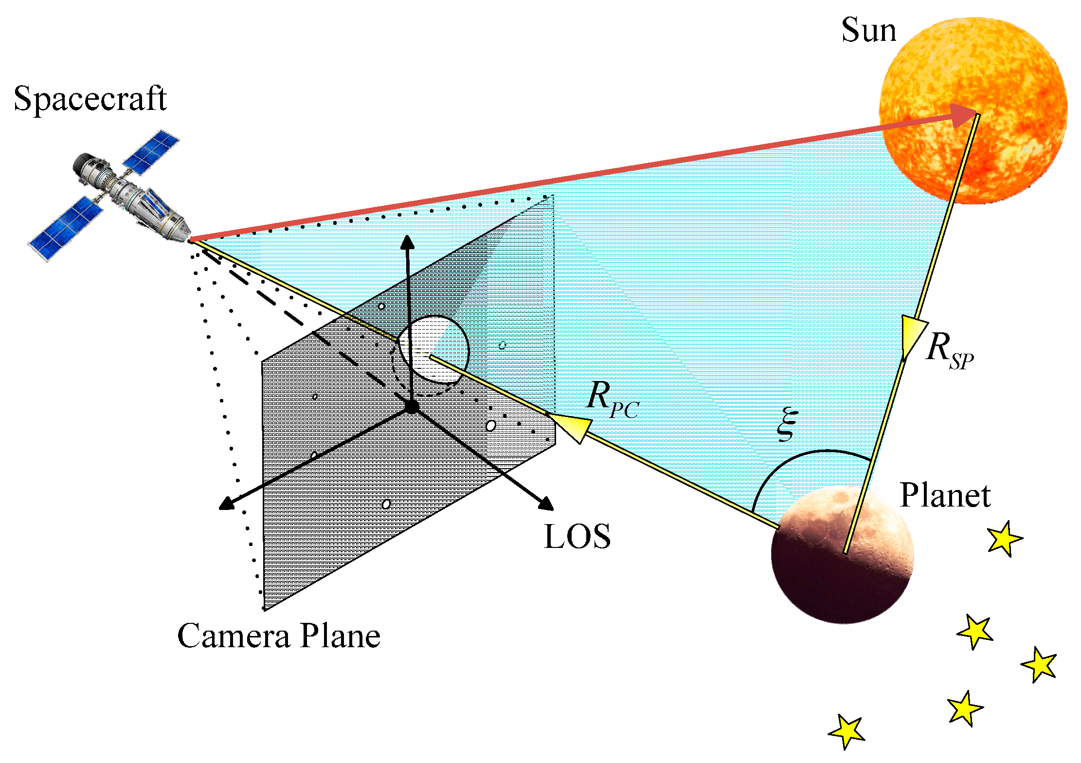
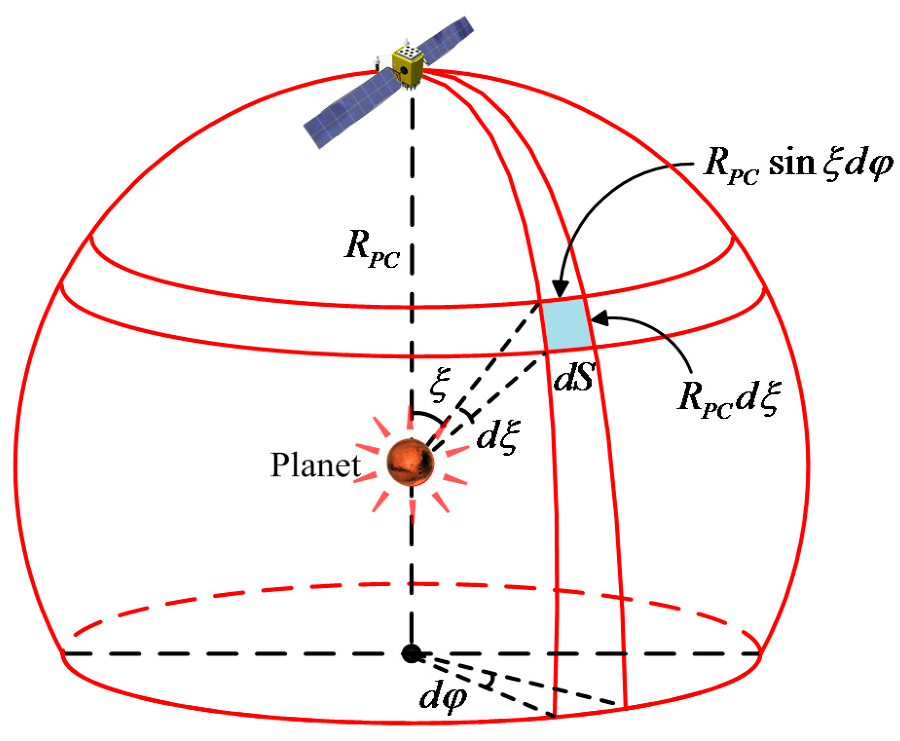
2. Irradiance Characteristics of a Celestial Body
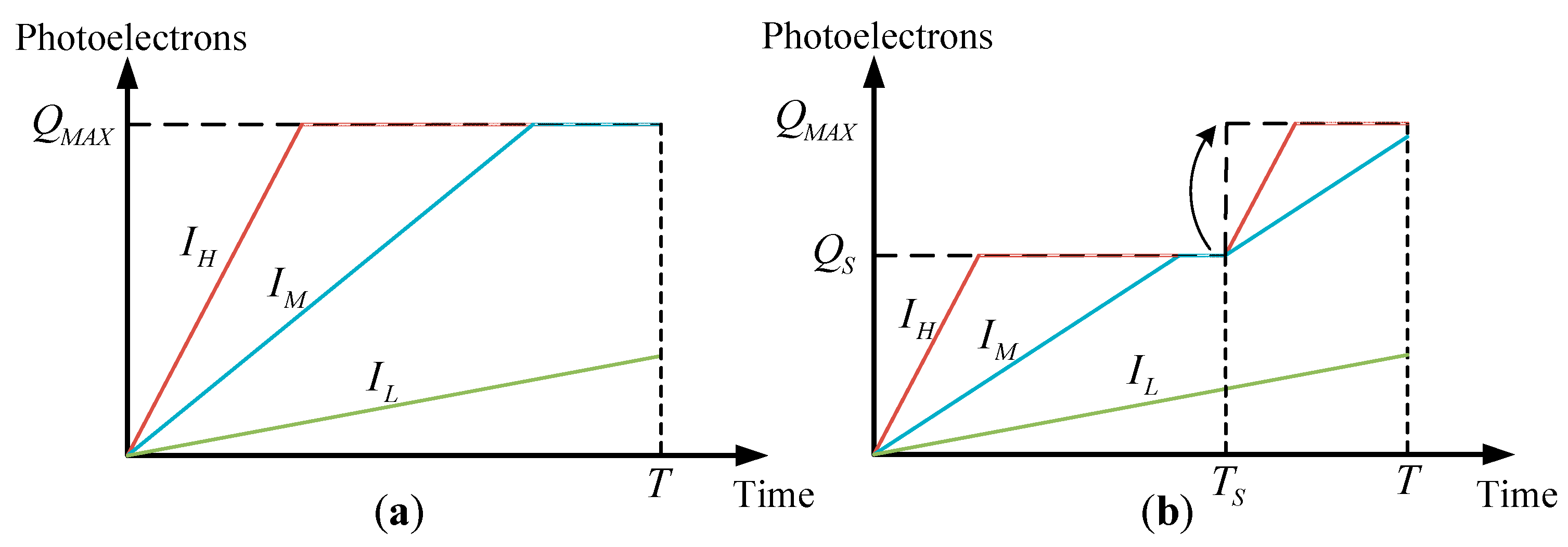
3. Celestial Object Imaging Model based on the Well Capacity Adjusting Scheme
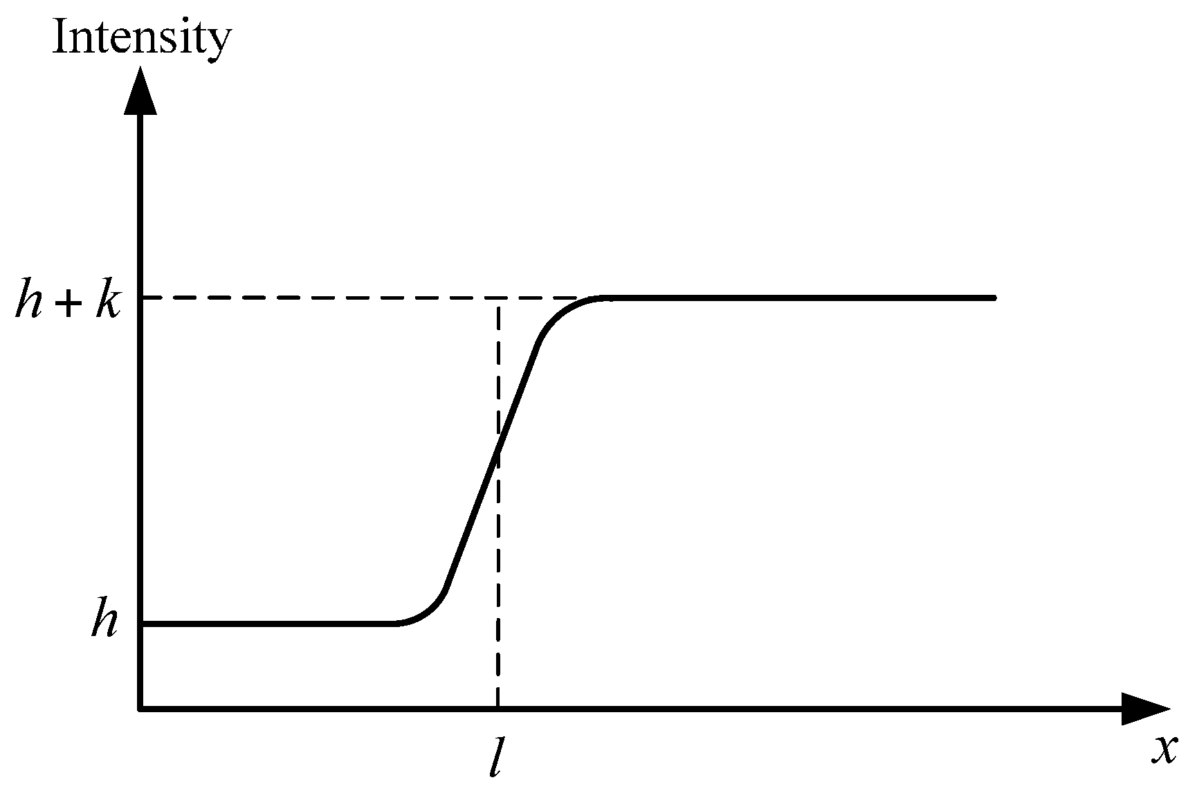
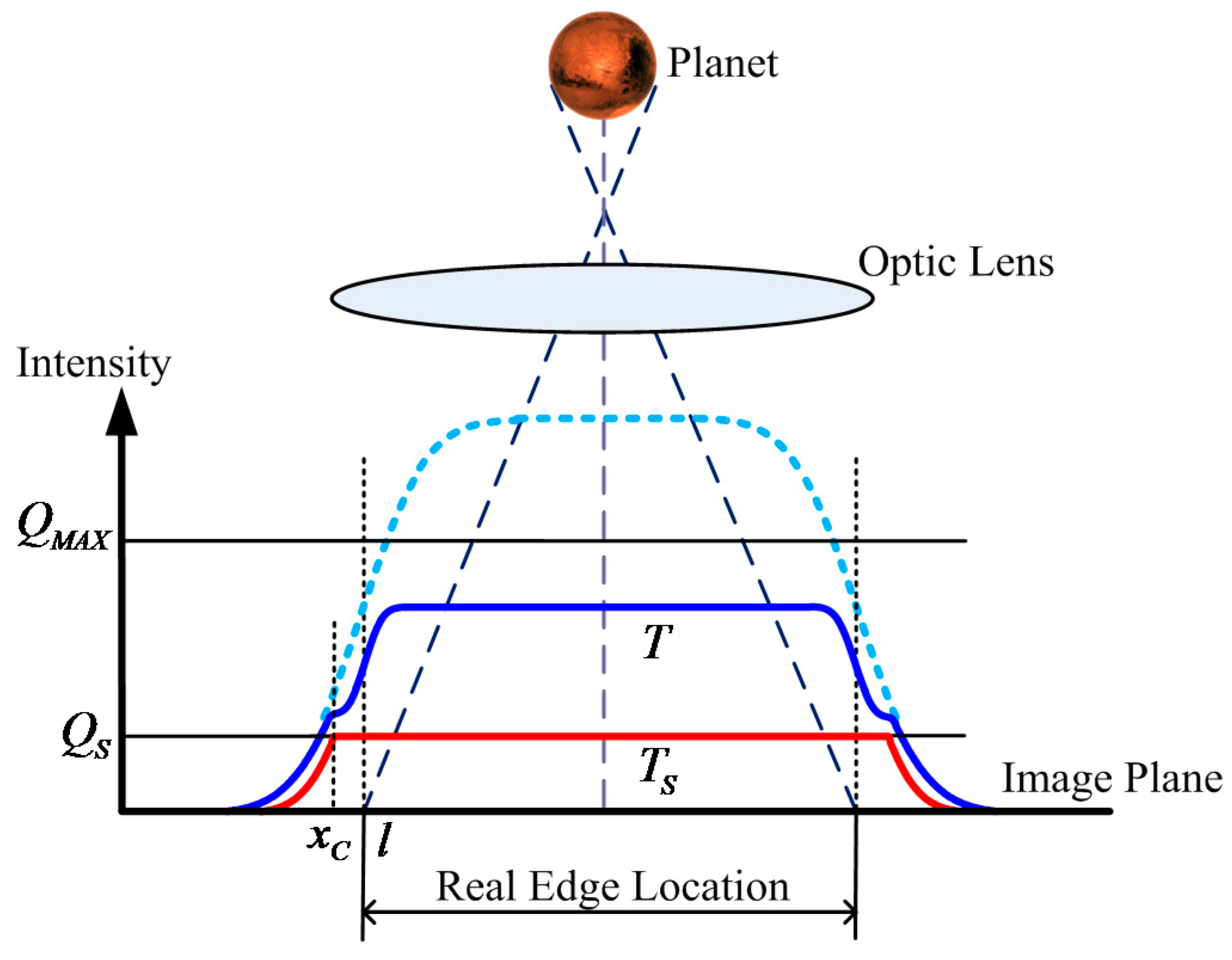
3.1. Celestial Body Edge Model
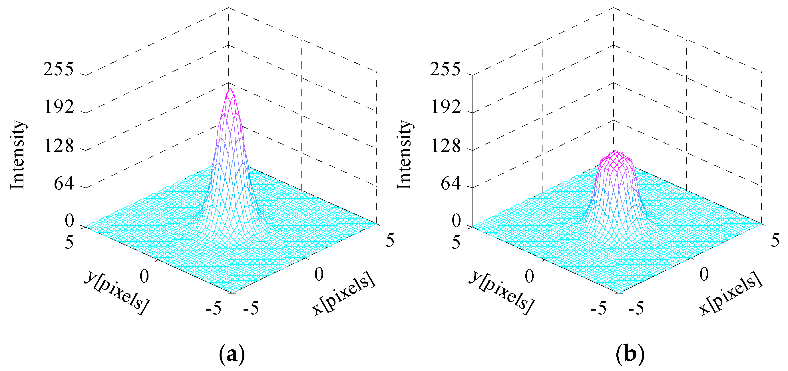
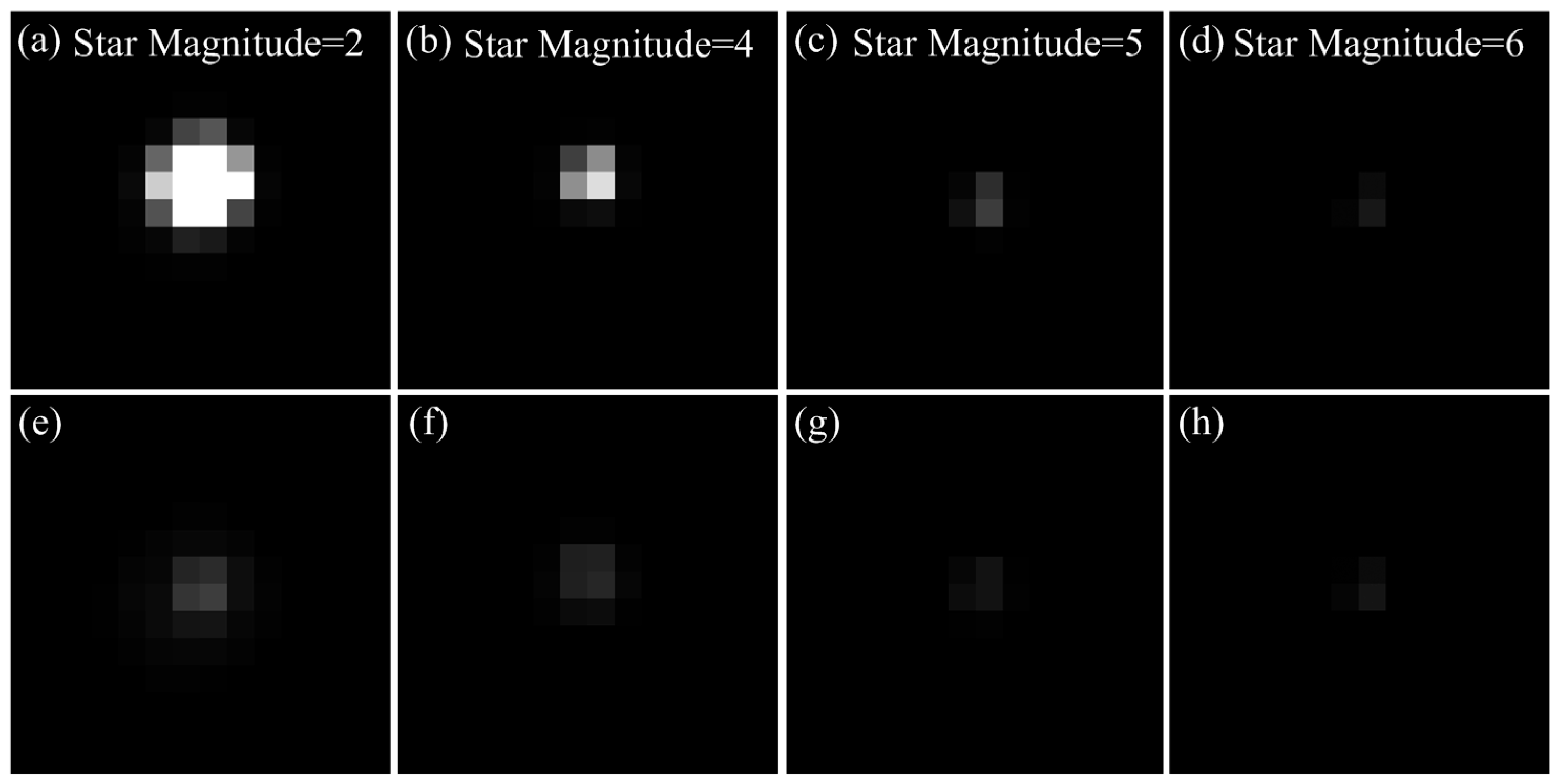
3.2. Star Spot Imaging Model
4. Celestial Object Image Feature Extraction Accuracy Performance Utilizing the WCA Scheme
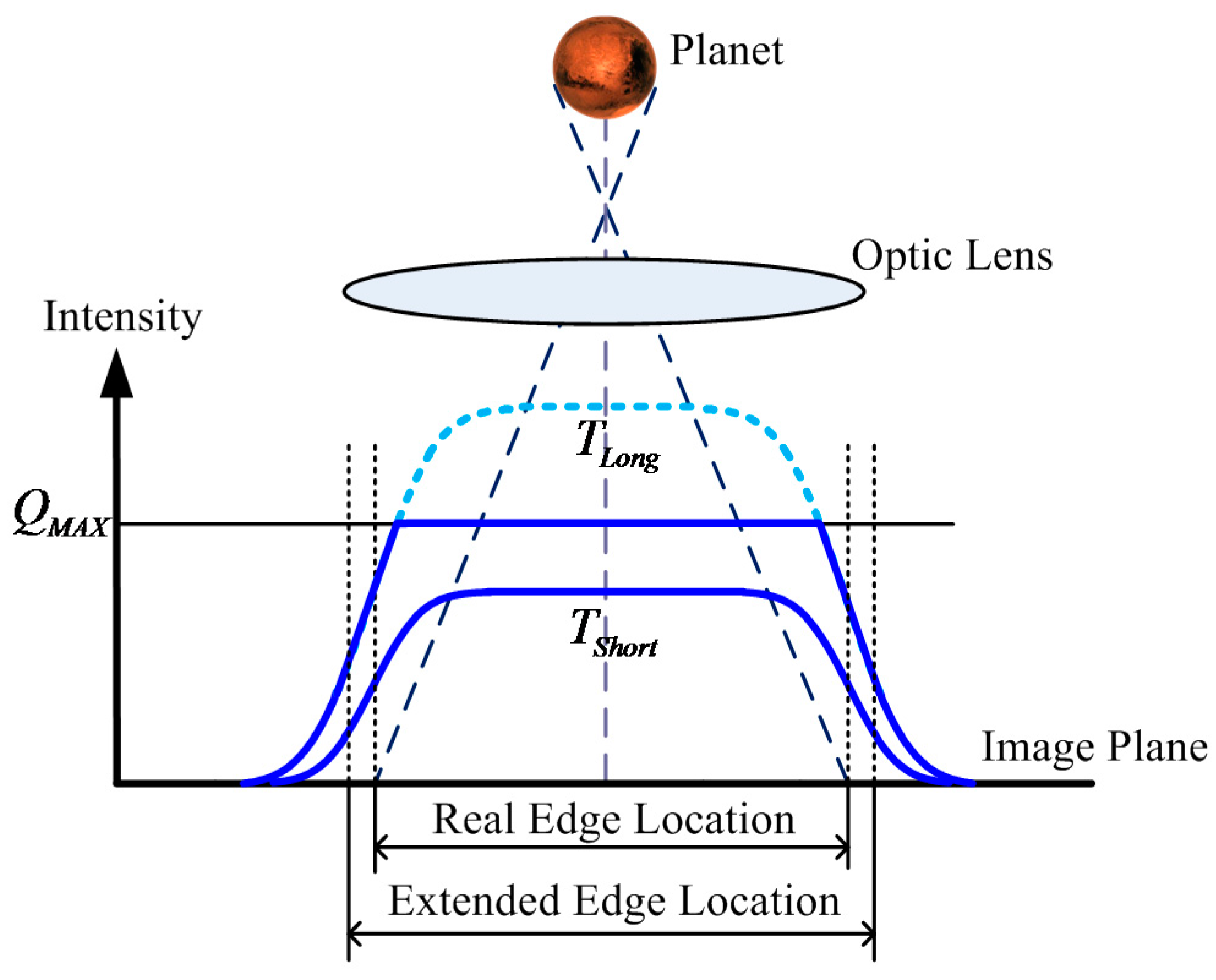
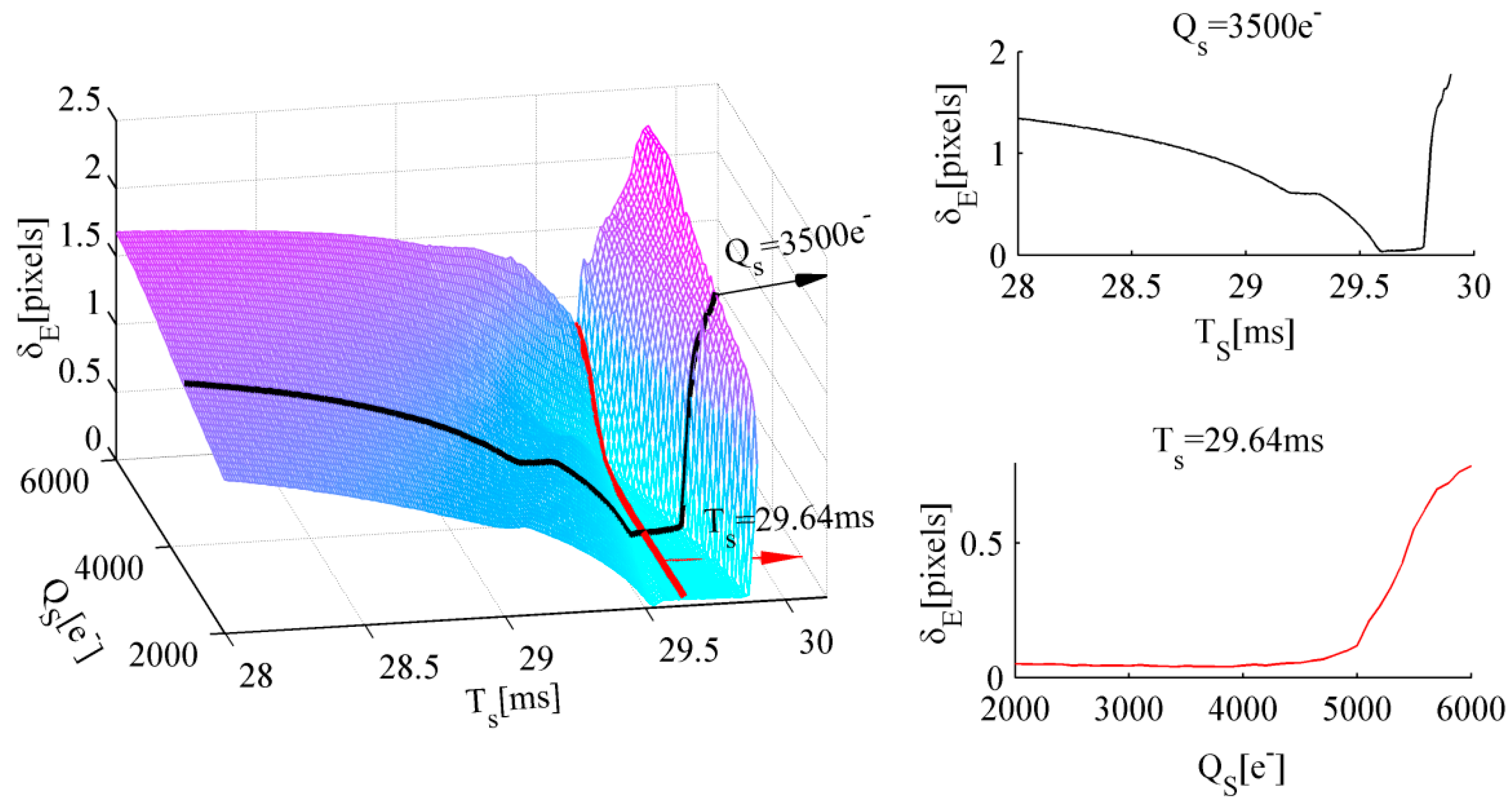
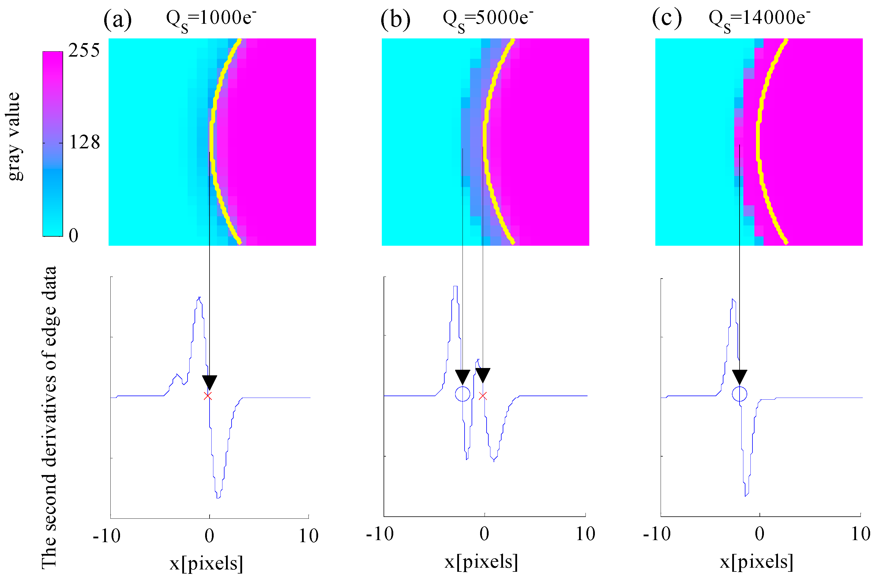
4.1. Edge Detection Accuracy Performance Utilizing the WCA Scheme
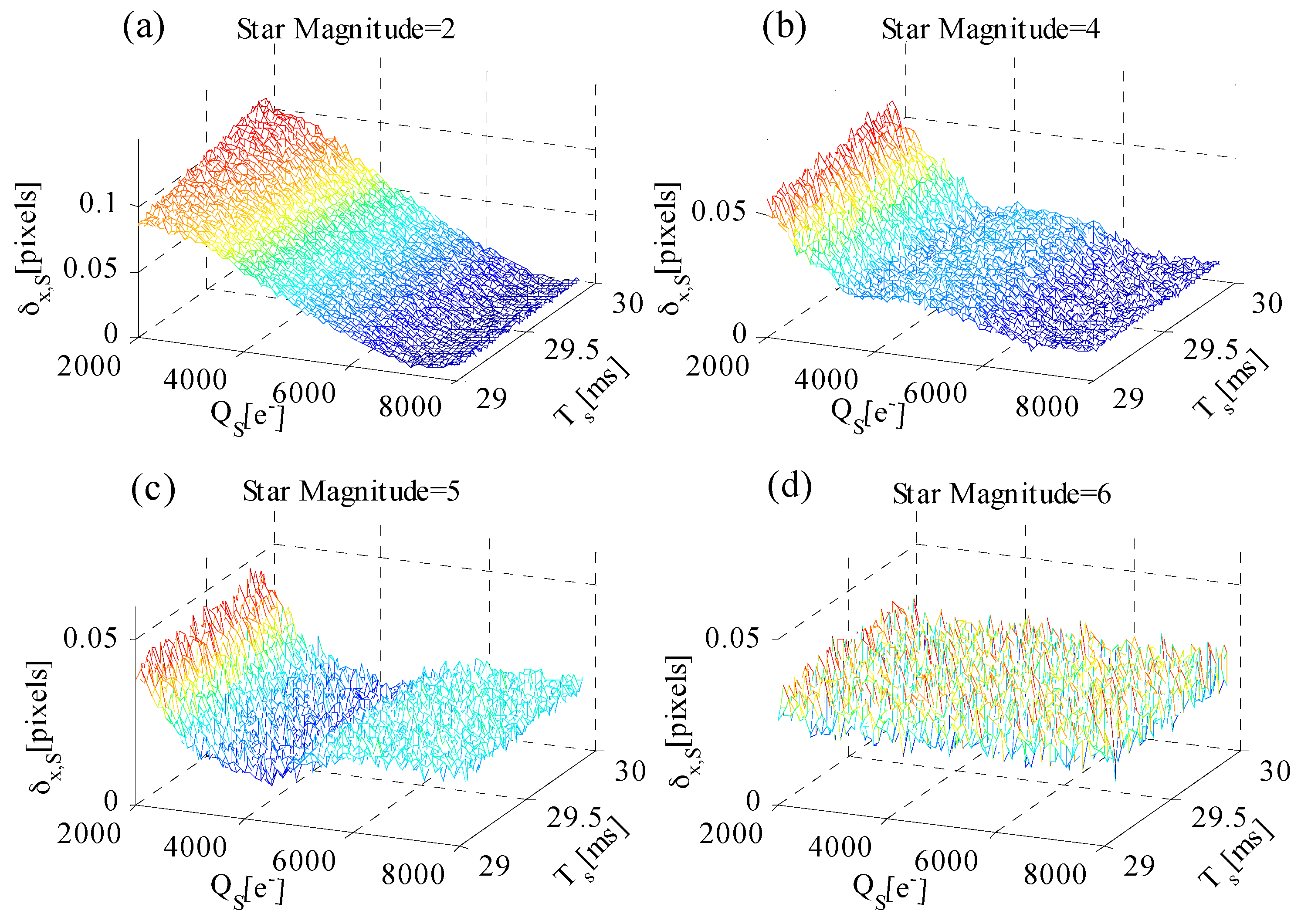
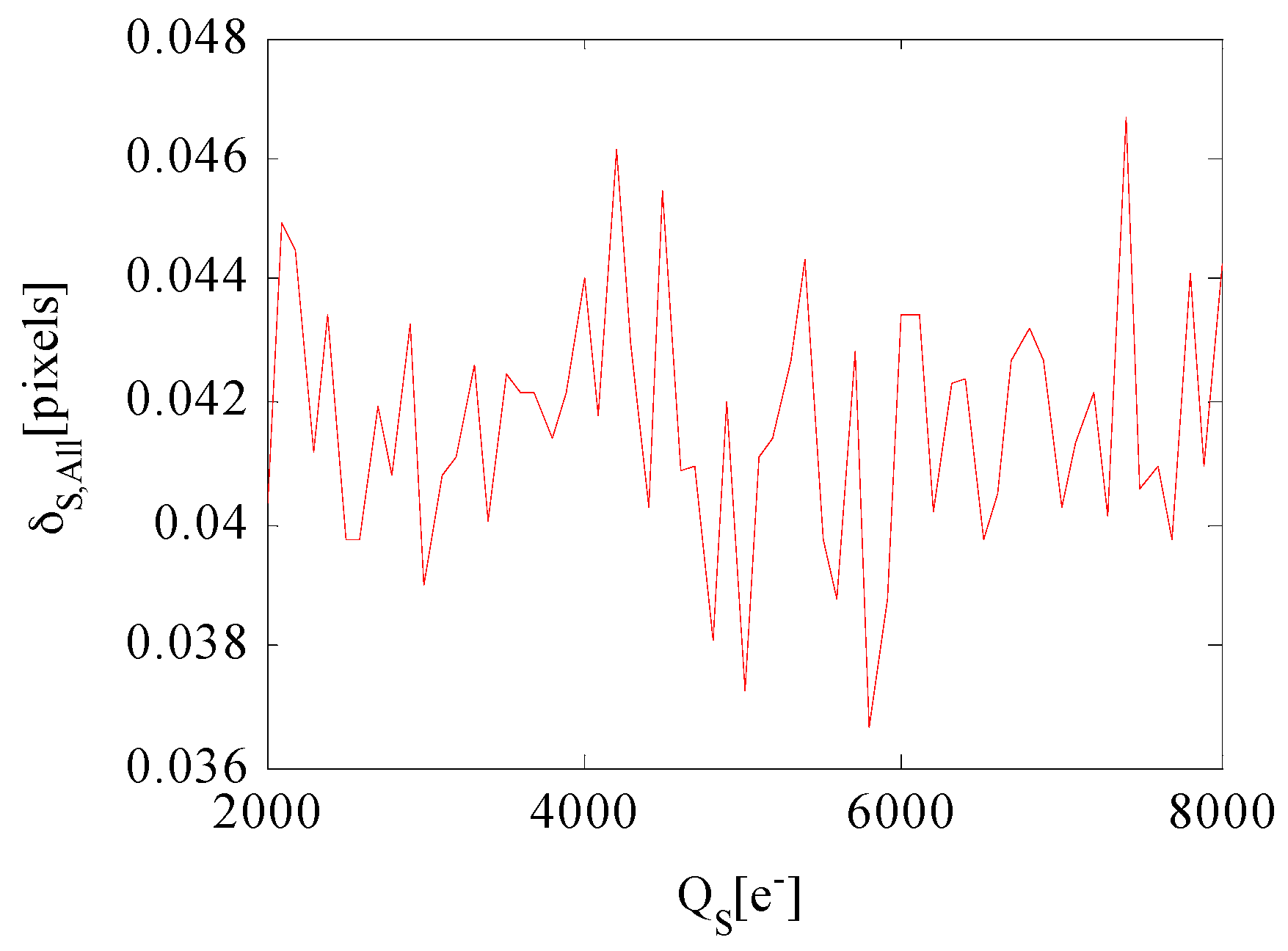
4.2. Star Centroiding Accuracy Performance Utilizing the WCA Scheme
5. Exposure Parameter Optimization
5.1. Total Integration Time
5.2. Adjusting Integration Time
5.3. Well Capacity
6. Experimental Results and Analysis
6.1. Laboratorial Single-Star Imaging and Accuracy Analysis Experiment
6.2. Night Sky Observation and Accuracy Analysis Experiment
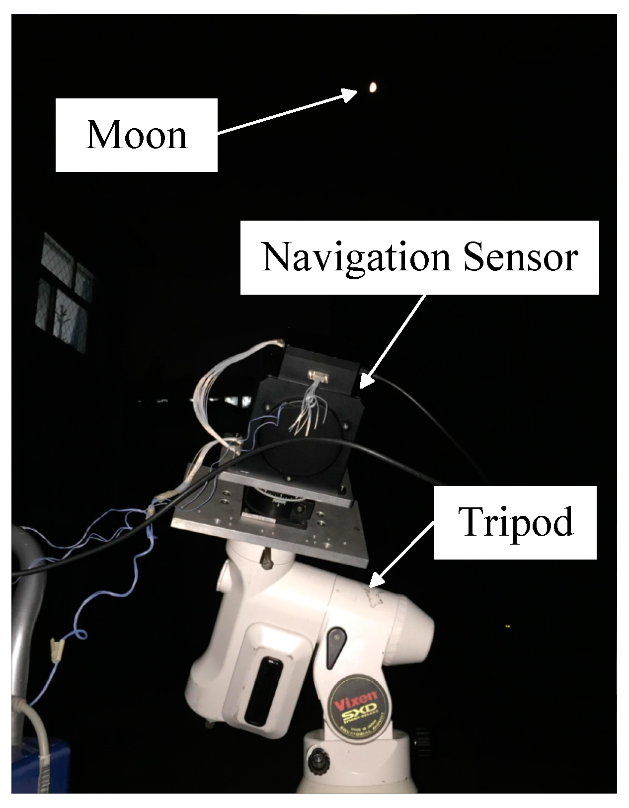
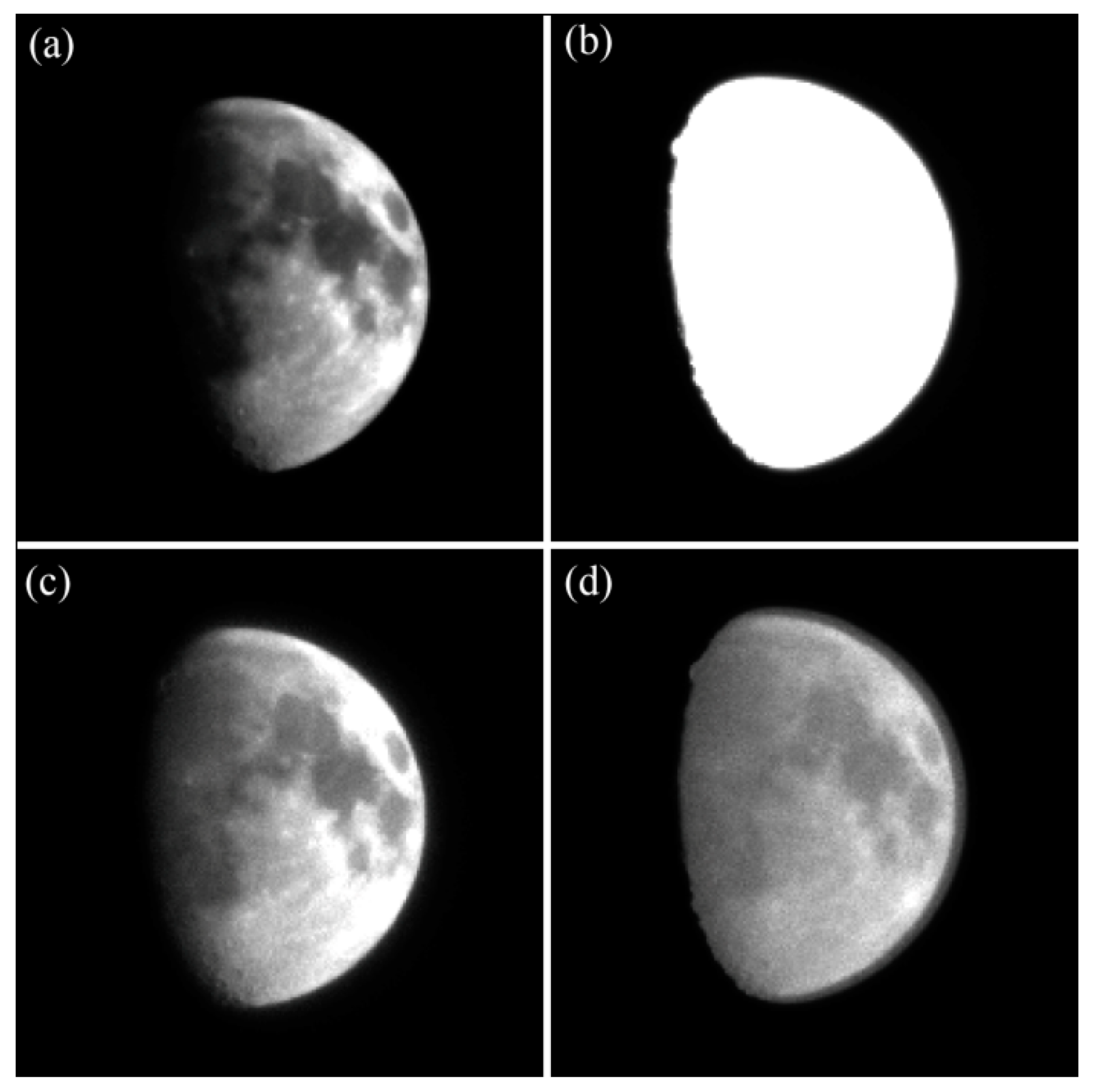
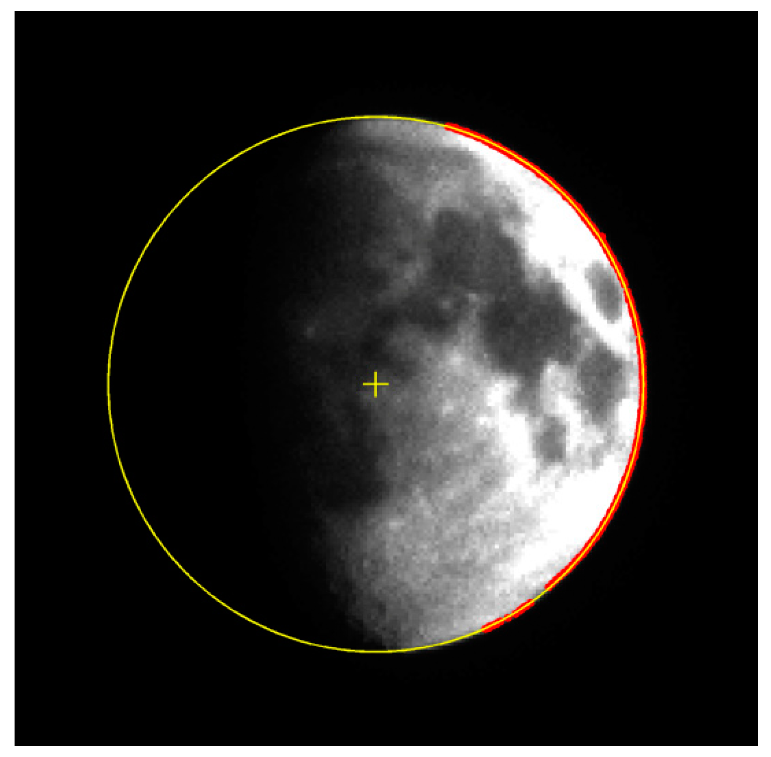
6.2.1. Observations of the Moon and Accuracy Analysis Experiment
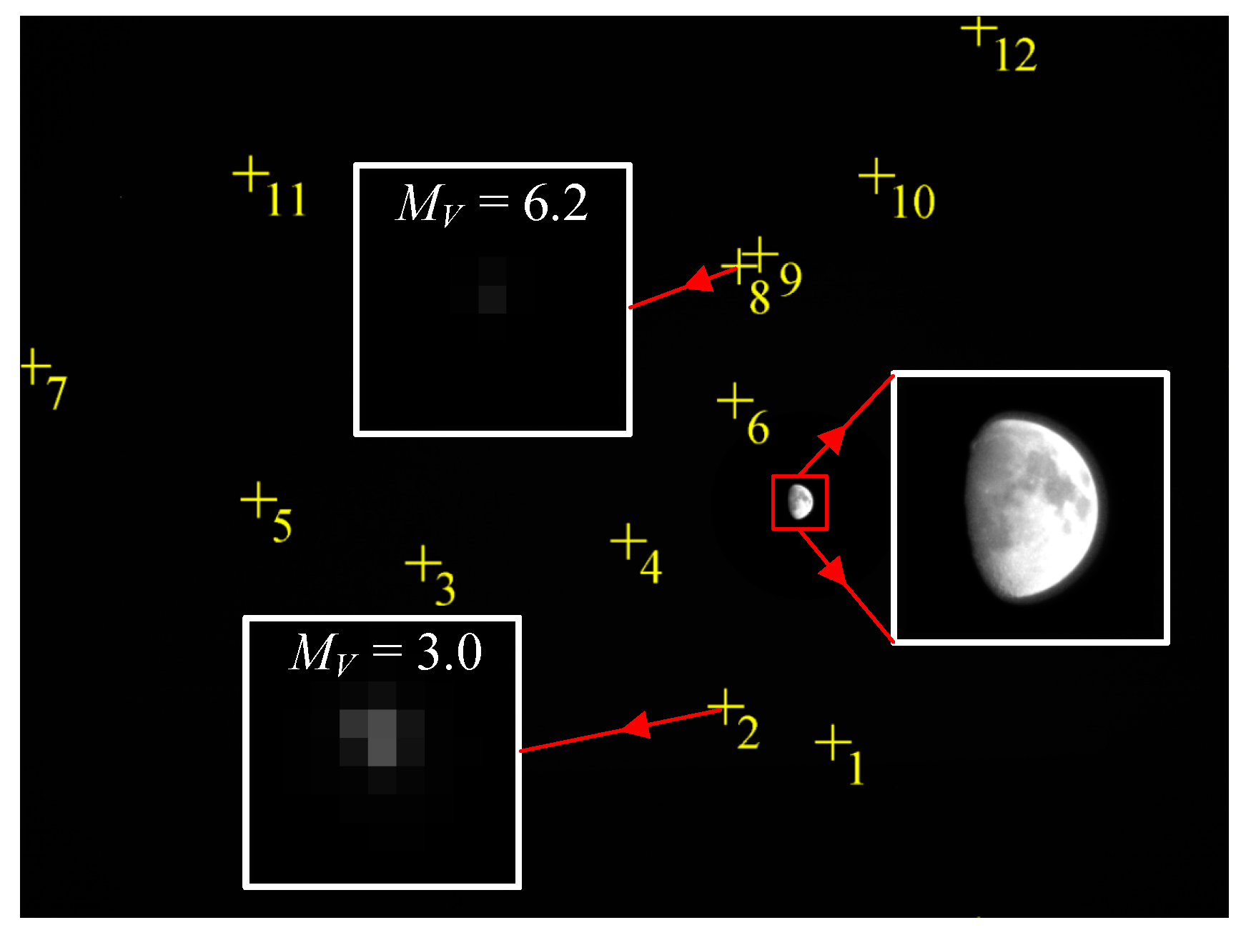
6.2.2. Observations of the Moon and Stars in the Same FOV
7. Conclusions
Acknowledgments
Author Contributions
Conflicts of Interest
References
- El Gamal, A.; Eltoukhy, H. CMOS image sensors. IEEE Circuits Devices Mag. 2005, 21, 6–20. [Google Scholar] [CrossRef]
- Kühl, C.T. Combined Earth-/Star Sensor for Attitude and Orbit Determination of Geostationary Satellites. Ph.D. Dissertation, Universität Stuttgart, Stuttgart, Baden-Württemberg, Germany, March 2005. [Google Scholar]
- Jinno, T.; Okuda, M. Multiple exposure fusion for high dynamic range image acquisition. IEEE Trans. Image Process. 2012, 21, 358–365. [Google Scholar] [CrossRef] [PubMed]
- Zhang, W.; Cham, W.-K. Reference-guided exposure fusion in dynamic scenes. J. Vis. Commun. Image Represent. 2012, 23, 467–475. [Google Scholar] [CrossRef]
- Goshtasby, A.A. Fusion of multi-exposure images. Image Vis. Comput. 2005, 23, 611–618. [Google Scholar] [CrossRef]
- Mertens, T.; Kautz, J.; Van Reeth, F. Exposure fusion: A simple and practical alternative to high dynamic range photography. In Computer Graphics Forum; Blackwell Publishing Ltd.: Oxford, UK, 2009; Volume 28, pp. 161–171. [Google Scholar]
- Yang, D.X.; El Gamal, A. Comparative analysis of SNR for image sensors with enhanced dynamic range. In Sensors, Cameras, and Systems for Scientific/Industrial Applications; Blouke, M.M., Williams, G.M., Jr., Eds.; SPIE: San Jose, CA, USA, 1999; Volume 3649, pp. 197–211. [Google Scholar]
- Cheng, H.-Y.; Choubey, B.; Collins, S. An integrating wide dynamic-range image sensor with a logarithmic response. IEEE Trans. Electron Devices 2009, 56, 2423–2428. [Google Scholar] [CrossRef]
- Kavadias, S.; Dierickx, B.; Scheffer, D.; Alaerts, A.; Uwaerts, D.; Bogaerts, J. A logarithmic response CMOS image sensor with on-chip calibration. IEEE J. Solid State Circuits 2000, 35, 1146–1152. [Google Scholar] [CrossRef]
- Kim, D.; Song, M. An enhanced dynamic-range CMOS image sensor using a digital logarithmic single-slope ADC. IEEE Trans. Circuits Syst. II Express Briefs 2012, 59, 653–657. [Google Scholar] [CrossRef]
- Brajovic, V.; Kanade, T. A sorting image sensor: An example of massively parallel intensity-to-time processing for low-latency computational sensors. In Proceedings of the IEEE International Conference on Robotics and Automation, Minneapolis, MN, USA, 22–28 April 1996; pp. 1638–1643. [Google Scholar]
- Luo, Q.; Harris, J.G.; Chen, Z.J. A time-to-first spike CMOS image sensor with coarse temporal sampling. Analog Integr. Circuits Signal Process. 2006, 47, 303–313. [Google Scholar] [CrossRef]
- Stoppa, D.; Simoni, A.; Gonzo, L.; Gottardi, M.; Dalla Betta, G.-F. Novel CMOS image sensor with a 132-dB dynamic range. IEEE J. Solid State Circuits 2002, 37, 1846–1852. [Google Scholar] [CrossRef]
- Stoppa, D.; Vatteroni, M.; Covi, D.; Baschirotto, A.; Sartori, A.; Simoni, A. A 120-dB dynamic range CMOS image sensor with programmable power responsivity. IEEE J. Solid State Circuits 2007, 42, 1555–1563. [Google Scholar] [CrossRef]
- Knight, T.F. Design of an Integrated Optical Sensor with on-Chip Preprocessing. Ph.D. Dissertation, Massachusetts Institute of Technology, Cambridge, MA, USA, 1983. [Google Scholar]
- Sayag, M. Non-Linear Photosite Response in CCD Imagers. U.S. Patent No. 5,055,667, 8 October 1991. [Google Scholar]
- Decker, S.; McGrath, D.; Brehmer, K.; Sodini, C.G. A 256 × 256 CMOS imaging array with wide dynamic range pixels and column-parallel digital output. IEEE J. Solid State Circuits 1998, 33, 2081–2091. [Google Scholar] [CrossRef]
- Fossum, E.R. High Dynamic Range Cascaded Integration Pixel Cell and Method of Operation. U.S. Patent No. 6,888,122, 3 May 2005. [Google Scholar]
- Akahane, N.; Sugawa, S.; Adachi, S.; Mori, K.; Ishiuchi, T.; Mizobuchi, K. A sensitivity and linearity improvement of a 100-dB dynamic range CMOS image sensor using a lateral overflow integration capacitor. IEEE J. Solid State Circuits 2006, 41, 851–858. [Google Scholar] [CrossRef]
- Lee, W.; Akahane, N.; Adachi, S.; Mizobuchi, K.; Sugawa, S. A high S/N ratio and high full well capacity CMOS image sensor with active pixel readout feedback operation. In Proceedings of the Solid-State Circuits Conference, ASSCC’07, IEEE Asian, Jeju City, Korea, 12–14 Novmber 2007; pp. 260–263. [Google Scholar]
- Hawkins, S.E., III; Boldt, J.D.; Darlington, E.H.; Espiritu, R.; Gold, R.E.; Gotwols, B.; Grey, M.P.; Hash, C.D.; Hayes, J.R.; Jaskulek, S.E. The Mercury dual imaging system on the MESSENGER spacecraft. Space Sci. Rev. 2007, 131, 247–338. [Google Scholar] [CrossRef]
- Iqbal, M. An Introduction to Solar Radiation, 1st ed.; Academic Press: Don Mills, ON, Canada, 2012; pp. 35–36. [Google Scholar]
- The Information of Bond Albedo. Available online: https://en.wikipedia.org/wiki/Bond_albedo (accessed on 9 November 2016).
- Hagara, M.; Kulla, P. Edge detection with sub-pixel accuracy based on approximation of edge with Erf function. Radioengineering 2011, 20, 516–524. [Google Scholar]
- Lightsey, G.E.; Christian, J.A. Onboard image-processing algorithm for a spacecraft optical navigation sensor system. J. Spacecr. Rocket. 2012, 49, 337–352. [Google Scholar] [CrossRef]
- Steger, C. Unbiased Extraction of Curvilinear Structures from 2D and 3D Images. Ph.D. Dissertation, Technische Universität München, Arcisstraße 21, Munich, Bavaria, Germany, 1998. [Google Scholar]
- Liebe, C.C. Accuracy performance of star trackers-a tutorial. IEEE Trans. Aerosp. Electron. Syst. 2002, 38, 587–599. [Google Scholar] [CrossRef]


| Parameter | Value | Parameter | Value |
|---|---|---|---|
| Active pixels | PRNU | ||
| Pixel pitch | 6.4 μm × 6.4 μm | DSNU | |
| Full well capacity, | Read noise | ||
| Conversion gain | Quantization bits | 12 | |
| Dark current | Quantum efficiency, | 0.45 |
| Exposure Conditions | Apparent Radius/Pixels | Error/Pixels |
|---|---|---|
| Normal integration, | 71.44 | 0.42 |
| Normal integration, | 75.36 | 4.34 |
| WCA, | 71.46 | 0.44 |
| WCA, | 71.36 | 0.34 |
| WCA, | 71.60 | 0.58 |
| WCA, | 72.12 | 1.10 |
| Number | Centroid/Pixels | Magnitude | Number | Centroid/Pixels | Magnitude |
|---|---|---|---|---|---|
| 1 | (3439.886, 3084.843) | 3.8 | 7 | (57.533, 1493.233) | 4.9 |
| 2 | (2985.837, 2934.429) | 3.0 | 8 | (3045.821, 1069.692) | 6.2 |
| 3 | (1707.333, 2326.095) | 4.4 | 9 | (3131.244, 1017.171) | 5.3 |
| 4 | (2575.164, 2232.000) | 5.2 | 10 | (3624.311, 684.475) | 4.8 |
| 5 | (1012.179, 256.769) | 5.5 | 11 | (977.373, 675.311) | 4.3 |
| 6 | (3025.250, 1638.643) | 5.4 | 12 | (4056.727, 59.644) | 3.1 |
© 2017 by the authors. Licensee MDPI, Basel, Switzerland. This article is an open access article distributed under the terms and conditions of the Creative Commons Attribution (CC BY) license (http://creativecommons.org/licenses/by/4.0/).
Share and Cite
Wang, H.; Jiang, J.; Zhang, G. Celestial Object Imaging Model and Parameter Optimization for an Optical Navigation Sensor Based on the Well Capacity Adjusting Scheme. Sensors 2017, 17, 915. https://doi.org/10.3390/s17040915
Wang H, Jiang J, Zhang G. Celestial Object Imaging Model and Parameter Optimization for an Optical Navigation Sensor Based on the Well Capacity Adjusting Scheme. Sensors. 2017; 17(4):915. https://doi.org/10.3390/s17040915
Chicago/Turabian StyleWang, Hao, Jie Jiang, and Guangjun Zhang. 2017. "Celestial Object Imaging Model and Parameter Optimization for an Optical Navigation Sensor Based on the Well Capacity Adjusting Scheme" Sensors 17, no. 4: 915. https://doi.org/10.3390/s17040915
APA StyleWang, H., Jiang, J., & Zhang, G. (2017). Celestial Object Imaging Model and Parameter Optimization for an Optical Navigation Sensor Based on the Well Capacity Adjusting Scheme. Sensors, 17(4), 915. https://doi.org/10.3390/s17040915