
A Theoretical Study and Numerical Simulation of a Quasi-Distributed Sensor Based on the Low-Finesse Fabry-Perot Interferometer: Frequency-Division Multiplexing


Abstract
:1. Introduction
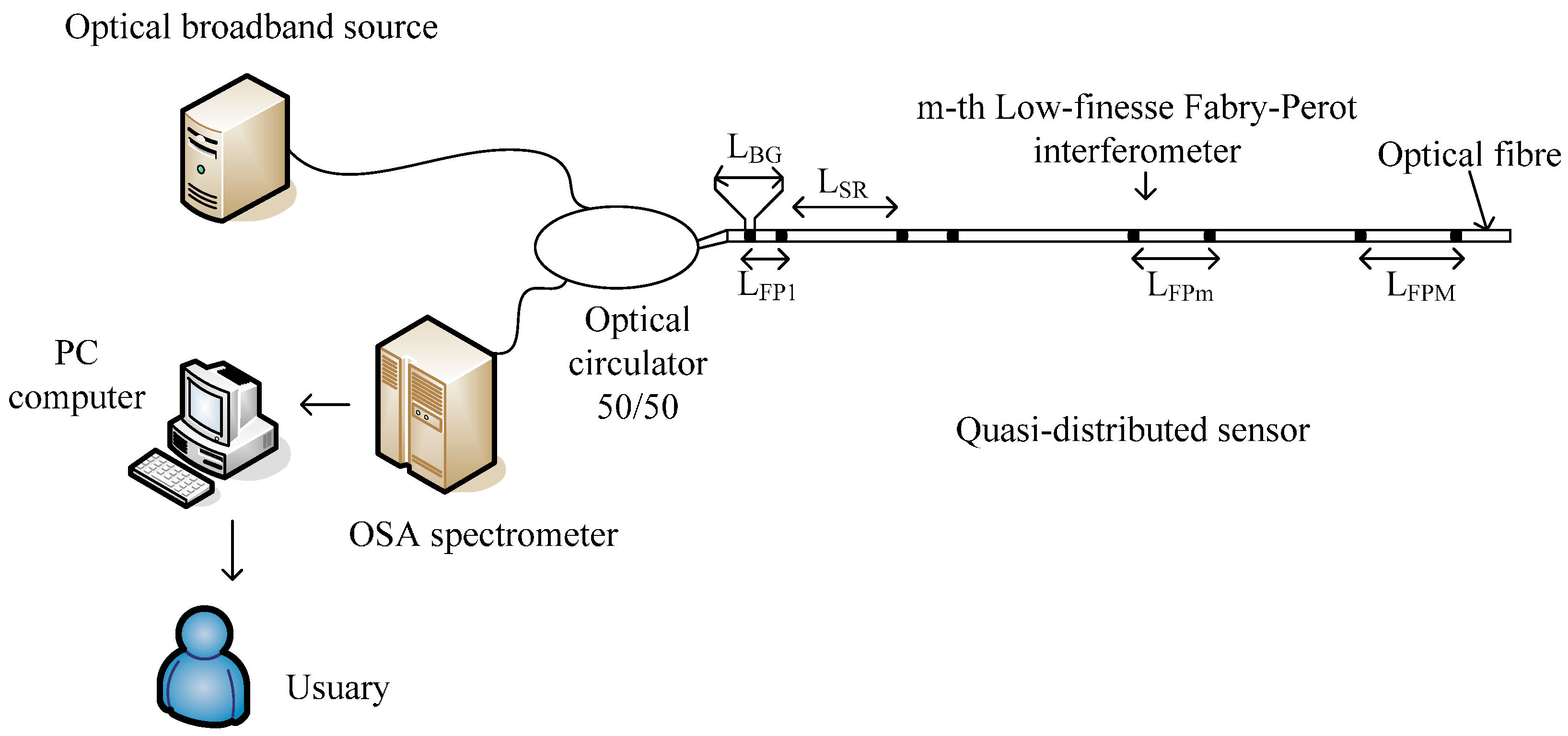
2. Optical Signal
2.1. and Spectrums
2.2. and Spectrums
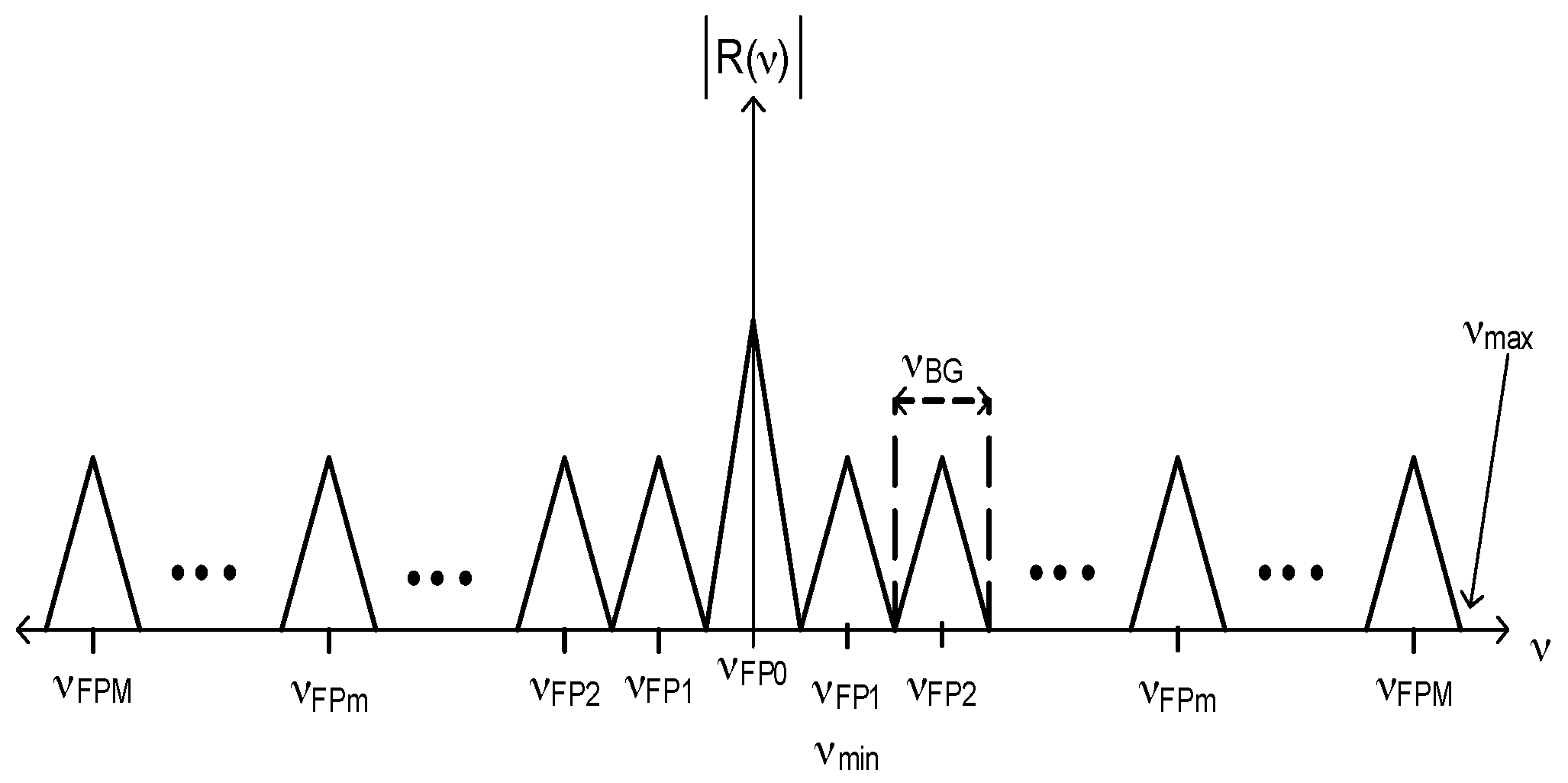
3. Cavity Length
3.1. Minimum Cavity Length
3.2. Maximum Cavity Length
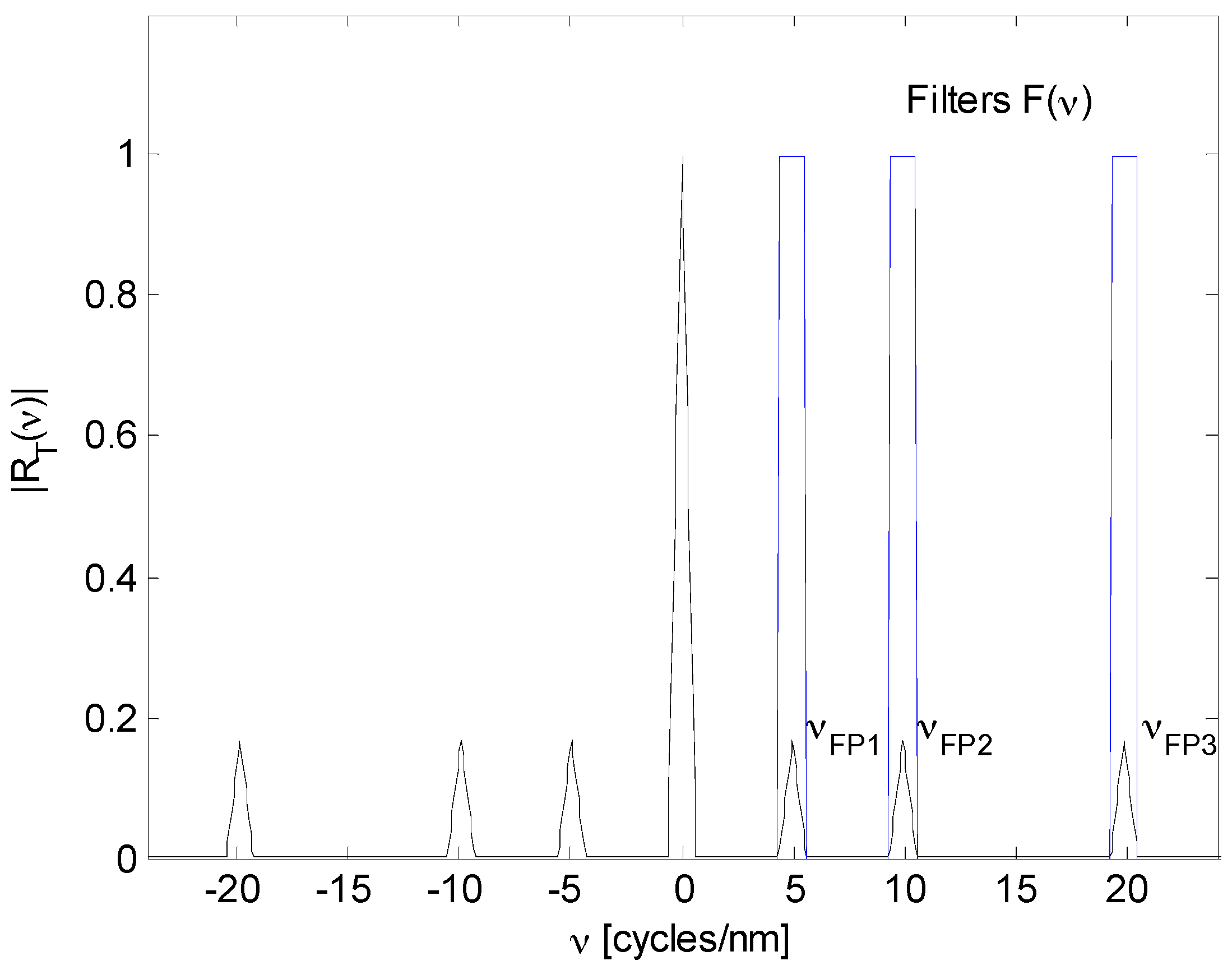
4. Capacity of Frequency-Division Multiplexing
5. Number of Samples
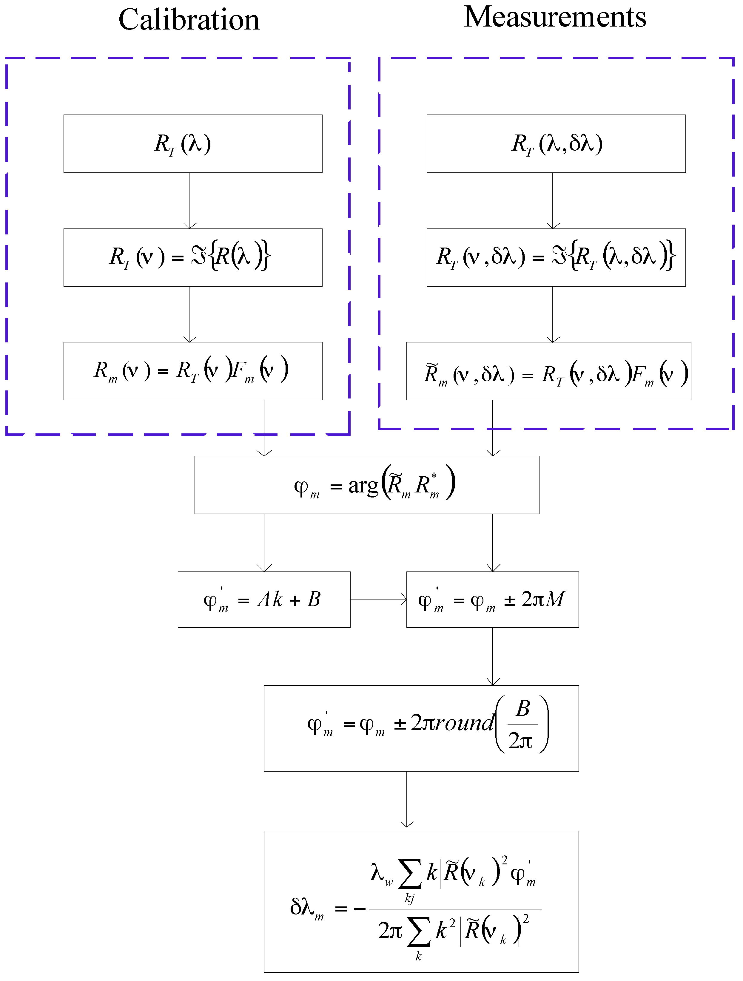
6. Digital Demodulation
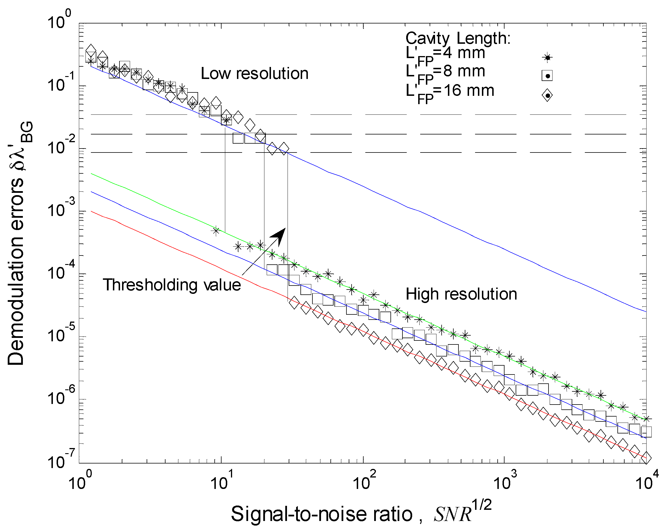
7. Numerical Simulation and Discussion
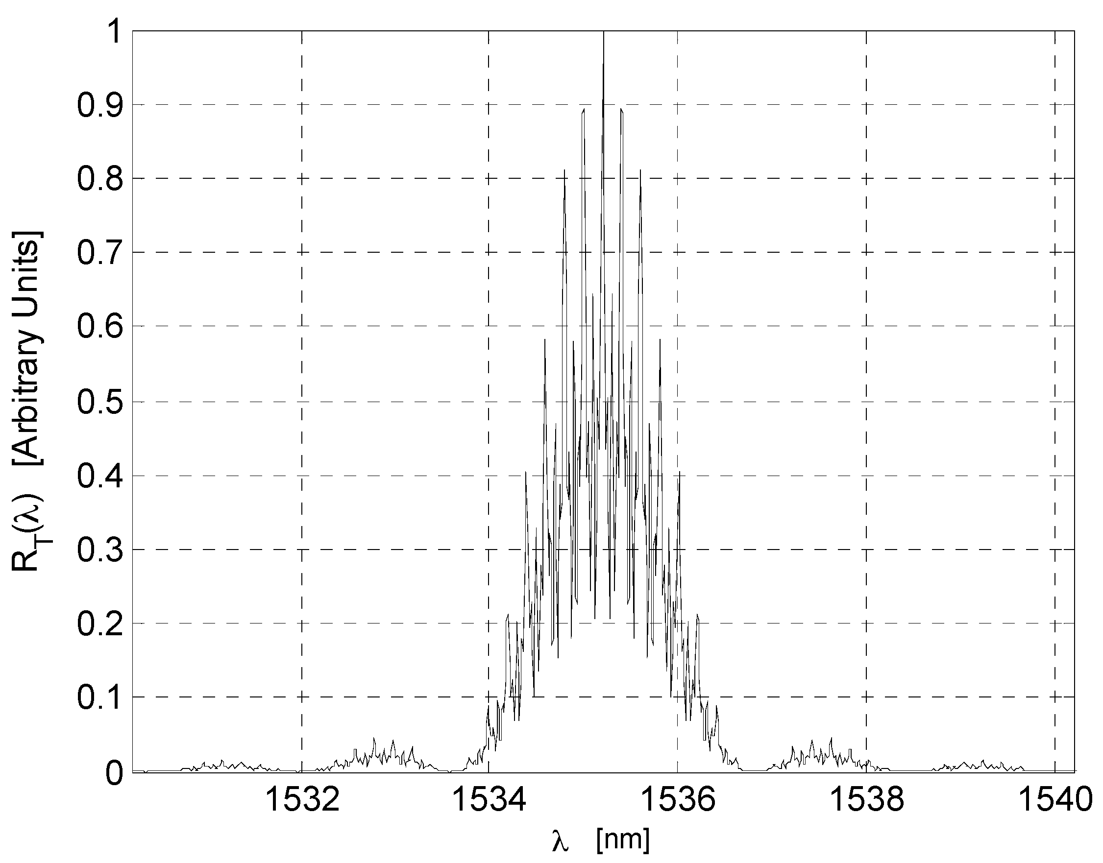
7.1. Parameters and Results
7.2. Discussion
8. Conclusions
Acknowledgments
Author Contributions
Conflicts of Interest
References
- Kashyap, R. Photosensitive Optical Fibers: Device and Applications. Opt. Fiber Technol. 1994, 1, 17–34. [Google Scholar] [CrossRef]
- Posada-Roman, J.E.; Garcia-Souto, J.A.; Poiana, D.A.; Acedo, P. Fast Interrogation of Fiber Bragg Gratins with Electro-Optical Dual Optical Frequency Combs. Sensors 2016, 16, 2007. [Google Scholar] [CrossRef] [PubMed]
- Di Sante, R. Fibre Optic Sensors for Structural Health Monitoring of Aircraft Composite Structures: Recent Advances and Applications. Sensors 2015, 15, 18666–18713. [Google Scholar] [CrossRef] [PubMed]
- Miridonov, S.V.; Shlyagin, M.G.; Spirin, V.V. Resolution limits and efficient signal processing for fiber optic Bragg grating sensors with direct spectroscopic detection. In Proceedings of the Optical Measurements Systems for Industrial Inspection III, Munich, Germany, 23–26 June 2003. [Google Scholar]
- Ben Zaken, B.B.; Zanzury, T.; Maka, D. An 8-Channel Wavelength MMI Demodultiplexer in Slot Waveguide Structures. Materials 2016, 9, 881. [Google Scholar] [CrossRef]
- Huang, J.; Zhou, Z.; Zhang, L.; Chen, J.; Ji, C.; Pham, T. Strain Modal Analysis of Small and Light Pipes Using Distributed Fibre Bragg Grating Sensors. Sensors 2016, 16, 1583. [Google Scholar] [CrossRef] [PubMed]
- Weng, Y.; Ip, E.; Pan, Z.; Wang, T. Advances Spatial-Division Multiplex Measurement Systems Propositions-From Telecommunication to Sensing Applications: A Review. Sensors 2016, 16, 1387. [Google Scholar] [CrossRef] [PubMed]
- Ali, T.A.; Shehata, M.I.; Mohamed, N.A. Design and performance investigation of a highly accurate apodized fiber Bragg grating-based strain sensors in single and quasi-distributed systems. Appl. Opt. 2015, 16, 5243–5251. [Google Scholar] [CrossRef] [PubMed]
- Cibula, E.; Donlagic, D. In-line short cavity Fabry-Perot strain sensor for quasi distributed measurements utilizing standard OTDR. Opt. Express 2007, 15, 8719–8730. [Google Scholar] [CrossRef] [PubMed]
- Kežmah, M.; Ðonlagic, D. Multimode All-fiber quasi-distributed refractometer sensor array and cross-talk mitigation. Appl. Opt. 2007, 46, 4081–4091. [Google Scholar] [CrossRef] [PubMed]
- Werzinger, S.; Bergdolt, S.; Engelbrecht, R.; Torsten, T.; Schmauss, B. Quasi-Distributed Fiber Bragg Grating Sensing Using Stepped Incoherent Optical Frequency Domain Reflectometry. J. Lightwave Technol. 2016, 34, 5270–5277. [Google Scholar] [CrossRef]
- Yu, Z.; Yang, J.; Yuan, Y.; Li, C.; Liang, S.; Hou, L.; Peng, F.; Wu, B.; Zhang, J.; Liu, Z.; Yuan, L. Quasi-distributed birefringence dispersion measurement for polarization maintain device with high accuracy based on white light interferometry. Opt. Express 2016, 24, 1587–1597. [Google Scholar] [CrossRef] [PubMed]
- Han, M.; Wang, A. Exact analysis of low-finesse multimode fiber extrinsic Fabry-Perot interferometers. Appl. Opt. 2004, 43, 4659–4666. [Google Scholar] [CrossRef] [PubMed]
- Beard, P.C.; Mils, T.N. Extrinsic optical-fiber ultrasound sensor using a thin polymer films as a low-finesse Fabry-Perot interferometer. Appl. Opt. 1996, 35, 663–675. [Google Scholar] [CrossRef] [PubMed]
- Town, G.E.; Sugden, K.; Williams, J.A.; Bennion, I.; Poole, S.B. Wide-Band Fabry-Perot-Like Filters in optical fiber. IEEE Photonics Technol. Lett. 1995, 7, 78–90. [Google Scholar] [CrossRef]
- Heredero, R.L.; Santos, J.L.; Fernádez de Celaya, R.; Guerrero, H. Micromachined low-finesse Fabry-Pérot interferometer for the measurement od DC and AC electrical currents. IEEE Sens. J. 2003, 3, 13–18. [Google Scholar] [CrossRef]
- Ferreira, L.A.; Lobo Ribeiro, A.B.; Santos, J.L.; Farahi, F. Simultaneous measurements of displacement and temperature using a low finesse cavity and fiber Bragg grating. IEEE Photonics Technol. Lett. 1996, 8, 1519–1521. [Google Scholar] [CrossRef]
- Yan, L.; Gui, Z.; Wang, G.; An, Y.; Gu, J.; Zhang, M.; Liu, X.; Wang, Z.; Wang, G.; Jia, P. A micro bubble structure Based Fabry-Perot optical fiber strain sensor with high sensitivity and low-cost characteristics. Sensors 2017, 17, 555. [Google Scholar] [CrossRef] [PubMed]
- Hirsch, M.; Majchrowicz, D.; Wierzba, P.; Weber, M.; Bechelany, M.; Jędrzejewaska-Szczerska, M. Low-coherence interferometric fiber-optic sensors with potential applications as biosensors. Sensors 2017, 17, 261. [Google Scholar] [CrossRef] [PubMed]
- Betts, P.; Davis, J.A. Bragg grating Fabry-Perot interferometer with variable finesse. Opt. Eng. 2004, 43, 1258–1259. [Google Scholar] [CrossRef]
- Liang, W.; Huang, Y.; Xu, Y.; Lee, R.K.; Yariv, A. Highly sensitive fiber Bragg grating refractive index sensors. Appl. Phys. Lett. 2005, 86. [Google Scholar] [CrossRef]
- Kersey, A.D.; Berkoff, T.A. Fiber-optic Bragg-Grating Differential-Temperature sensor. IEEE Photonics Technol. Lett. 1992, 4, 1183–1185. [Google Scholar] [CrossRef]
- Zhang, M.; Sun, Q.; Wang, Z.; Li, X.; Liu, H.; Liu, D. A large capacity sensing network with identical weak fiber Bragg gratings multiplexing. Opt. Commun. 2012, 285, 3082–3087. [Google Scholar] [CrossRef]
- Xu, P.; Pang, F.; Chen, N.; Chen, Z.; Wang, T. Fabry-Perot temperature sensors for quasi-distributed measurement utilizing OTDR. J. Electron. Sci. Technol. China 2008, 6, 393–395. [Google Scholar]
- Zhao, Y.; Ansari, F. Quasi-distributed white light fiber optic strain sensor. Opt. Commun. 2001, 196, 133–137. [Google Scholar] [CrossRef]
- He, H.; Shao, L.Y.; Luo, B.; Zou, X.; Zhang, Z.; Pan, W.; Yan, L. Multiple vibration measurement using phase-sensitive OTDR merged with Mach-Zehnder interferometer based on frequency division multiplexing. Opt. Express 2016, 24, 10240–10247. [Google Scholar] [CrossRef]
- Miridonov, S.V.; Shlyaing, M.G.; Tentori, D. Twin-grating fiber optic sensor demodulation. Opt. Commun. 2001, 191, 253–262. [Google Scholar] [CrossRef]
- Shlyagin, M.G.; Swart, P.L.; Miridonov, S.V.; Chtcherbakov, A.A.; Márquez Borbon, I.; Spirin, V.V. Static strain measurement with sub-micro-strain resolution and large dynamic range using a twin-Bragg-grating Fabry-Perot sensor. Opt. Eng. 2002, 41, 1809–1814. [Google Scholar]
- Shlyagin, M.G.; Miridonov, S.V.; Tentori, D. Frequency multiplexing of in-fiber Bragg grating sensors using tunable laser. In Proceedings of the Micro-Optical for Measurement, Sensors, and Microsystems II and Optical Fiber Sensor Technologies and Applications, Munich, Germany, 24 September 1997; Volume 3099, p. 348. [Google Scholar]
- Shlyagin, M.G.; Miridonov, S.V.; Márquez-Borbón, I.; Spirin, V.V.; Swart, P.L.; Chtcherbakov, A.A. Multiplexed twin Bragg grating interferometer sensor. In Proceedings of the Optical Fiber Sensors Conference Technical Digest (OFS 2002), Portland, OR, USA, 10 May 2002; pp. 191–194. [Google Scholar]
- Trontz, A.; Cheng, B.; Zeng, S.; Xiao, H.; Dong, J. Development of Metal-Ceramic Coaxial Cable Fabry-Perot Interferometer Sensors for High Temperature Monitoring. Sensors 2015, 15, 24914–24925. [Google Scholar] [CrossRef] [PubMed]
- Li, X.; Sun, Q.; Liu, D.; Liang, R.; Zhang, J.; Wo, J.; Shum, P.P.; Liu, D. Simultaneous wavelength and frequency encoded microstructure based quasi-distributed temperature sensor. Opt. Express 2012, 20, 12076–12084. [Google Scholar] [CrossRef] [PubMed]
- Tao, Y.J.; Ran, Z.L.; Zhou, C.X. Fiber-optic Fabry-Perot sensors based on a combination of spatial-frequency division multiplexing and wavelength division multiplexing formed by chirped fiber Bragg grating pairs. Appl. Opt. 2006, 45, 5815–5818. [Google Scholar]
- Rao, Y.J.; Henderson, P.J.; Jackson, D.A.; Zhang, L.; Bennion, I. Simultaneous strain, temperature and vibration measurement using a multiplexed in-fibre-Bragg-grating/fibre-Fabry-Perot sensor system. Electron. Lett. 1997, 33, 2063–2064. [Google Scholar] [CrossRef]
- Martinez-Manuel, R.; Shlyagin, M.G.; Miridonov, S.V.; Meyer, J. Vibration Disturbance Localization Using a Serial Array of identical Low-Finesse Fiber Fabry-Perot Interferometers. IEEE Sens. 2012, 12, 124–127. [Google Scholar] [CrossRef]
- Viet Nguyen, L.; Vasiliev, M.; Alameh, K. Three-wave Fiber Fabry-Perot Interferometer for Simultaneous Measurement of Temperature and Water Salinity of Seawater. IEEE Photonics Technol. Lett. 2011, 23, 450–452. [Google Scholar] [CrossRef]
- Miridonov, S.V.; Shlyaing, M.G.; Tentori, D. Digital demodulation of twin-grating fiber-optic sensor. In Proceedings of the Conference on Fiber Optic and Laser Sensor and Application, Boston, MA, USA, 1 November 1998; Volume 3541, pp. 33–40. [Google Scholar]
- Shlyagin, M.G.; Miridonov, S.V.; Tentori Santa-Cruz, D.; Mendieta Jiménez, F.J.; Spirin, V.V. Multiplexing of grating-based fiber sensors using broadband spectral coding. In Proceedings of the Conference on Fiber Optic and Laser Sensors and Applications, Boston, MA, USA, 1 November 1998; Volume 3541, pp. 271–277. [Google Scholar]


| Sensor Number | Sensor Parameters | Signal Values |
|---|---|---|
| Low-finesse Fabry-Perot interferometer 1 (S1) | LFP1 = 4 [mm] | [nm] (Equation (3)) [Ciclos/nm] (Equation (4)) [Ciclos/nm] (Equation (9)) |
| LBG = 0.5 [mm] | ||
| n = 1.46 | ||
| [nm] | ||
| Low-finesse Fabry-Perot interferometer 2 (S2) | LFP2 = 8 [mm] | [nm] (Equation (3)) [Ciclos/nm] (Equation (4)) [Ciclos/nm] (Equation (9)) |
| LBG = 0.5 [mm] | ||
| n = 1.46 | ||
| [nm] | ||
| Low-finesse Fabry-Perot interferometer 3 (S3) | LFP3 = 16 [mm] | [nm] (Equation (3)) [Ciclos/nm] (Equation (4)) [Ciclos/nm] (Equation (9)) |
| LBG = 0.5 [mm] | ||
| n = 1.46 | ||
| [nm] |
| Parameters | Value | Equation |
|---|---|---|
| 1 [mm] | Equation (16) | |
| 40.2 [mm] | Equation (20) | |
| [mm] | Equation (21) | |
| 40 | Equations (23) and (24) | |
| 102.47 [Ciclos/nm] | Equation (25) | |
| 204.95 [Ciclos/nm] | Equation (26) |
© 2017 by the authors. Licensee MDPI, Basel, Switzerland. This article is an open access article distributed under the terms and conditions of the Creative Commons Attribution (CC BY) license (http://creativecommons.org/licenses/by/4.0/).
Share and Cite
Guillen Bonilla, J.T.; Guillen Bonilla, A.; Rodríguez Betancourtt, V.M.; Guillen Bonilla, H.; Casillas Zamora, A. A Theoretical Study and Numerical Simulation of a Quasi-Distributed Sensor Based on the Low-Finesse Fabry-Perot Interferometer: Frequency-Division Multiplexing. Sensors 2017, 17, 859. https://doi.org/10.3390/s17040859
Guillen Bonilla JT, Guillen Bonilla A, Rodríguez Betancourtt VM, Guillen Bonilla H, Casillas Zamora A. A Theoretical Study and Numerical Simulation of a Quasi-Distributed Sensor Based on the Low-Finesse Fabry-Perot Interferometer: Frequency-Division Multiplexing. Sensors. 2017; 17(4):859. https://doi.org/10.3390/s17040859
Chicago/Turabian StyleGuillen Bonilla, José Trinidad, Alex Guillen Bonilla, Verónica M. Rodríguez Betancourtt, Héctor Guillen Bonilla, and Antonio Casillas Zamora. 2017. "A Theoretical Study and Numerical Simulation of a Quasi-Distributed Sensor Based on the Low-Finesse Fabry-Perot Interferometer: Frequency-Division Multiplexing" Sensors 17, no. 4: 859. https://doi.org/10.3390/s17040859
APA StyleGuillen Bonilla, J. T., Guillen Bonilla, A., Rodríguez Betancourtt, V. M., Guillen Bonilla, H., & Casillas Zamora, A. (2017). A Theoretical Study and Numerical Simulation of a Quasi-Distributed Sensor Based on the Low-Finesse Fabry-Perot Interferometer: Frequency-Division Multiplexing. Sensors, 17(4), 859. https://doi.org/10.3390/s17040859