1. Introduction
The complexity related to the interacting subsystems of WT structures (namely the rotating blades, moving yaw mechanism, and pitch angle changes) and the alternating aerodynamic loads redefining the operational regime, result in a complex vibrating system necessitating adoption of efficient monitoring and diagnostic methods. The understanding of the intricate behavior of operating WT systems has preoccupied the research community since as early as the 1990s, resulting in development of operational modal analysis (OMA) methods, when in 1988 output-only testing was utilized for the first time on the 110 m high Éole turbine [
1]. Although directly related with the birth of the nowadays widely implemented OMA techniques, the assessment of WT infrastructure has still remained a multidisciplinary, rather challenging task. Moreover, with Europe’s strategic planning currently focusing on renewable energy management, WTs are resurging into the spotlight for both the industrial and research community [
2]. In this context, modern WT structures have to fulfil the growing demands for higher productivity and reduced downtime, which in turn calls for improved and automated SHM strategies, ensuring early-stage damage detection and structural diagnostics, reliability in power supply, as well as optimal operation and maintenance [
3,
4,
5,
6].
The difficulties related to assessment of operating WTs may be attributed among others sources to limited knowledge of the loading conditions (aeroelastic effects and rotor harmonics), the complexity of the multi-component WT system, varying operational regimes and environmental factors, as well as the typical uncertainties relating to incomplete and imperfect sensor data, modeling errors, complex and unique to the location soil-structure interaction effects.
Considering OMA methods applied on onshore operating WT structures, several studies based on short-term measurement campaigns successfully presented different concepts and novel measurement techniques [
7,
8,
9]. In more recent works implementation of long-term strategies for tracking variations in identified modal parameters has been reported, thus shifting the focus towards automated SHM schemes and interlinked fatigue assessment strategies [
10,
11,
12,
13,
14,
15]. In [
10] Devriendt et al. present an automated identification algorithm that combines an OMA tool (the poly-reference least squares complex frequency-domain estimator or covariance-driven stochastic subspace identification method) with a double clustering approach (hierarchical and fuzzy clustering algorithms). The proposed method is validated via successful tracking of minor changes in the dynamic behavior of an offshore wind turbine on data continuously collected during a two-week interval, for idling, i.e., parked, condition of the structure. Iliopoulos et al. [
11] propose and validate a response estimation methodology for acceleration predictions at arbitrary points of an offshore WT structure via fusion of a finite element model (FEM) of the structure, estimated OMA-based modal parameters and a limited number of measured acceleration time histories. In the work of Maes et al. [
12], a full-scale verification of three response estimation algorithms for the prediction of dynamic strains along the tower of an offshore monopile wind turbine is presented. The proposed hybrid filtering approaches combine a system model, derived from an updated FEM of the structure (based on OMA identification of the parked system), and a limited set of acceleration, and combined acceleration and strain measurements. The fatigue assessment strategy is verified for parked and rotating conditions of the structure. Male and Lourens in [
13] illustrated a strategy for real-time monitoring of WT fatigue accumulation by means of a joint input-state estimator. The method comprises of measuring operational vibrations at selected locations along a WT tower and strains assessment at unmeasured locations on the WT lattice support structure. The method is verified on artificial signals generated via a full-order FEM, whereas input forces and states are estimated on erroneous design model.
A significant point to keep in mind however is that the OMA class of methods is developed for implementation with time invariant systems [
16], while more refined schemes pertaining to non-stationary systems do exist but are less frequently applied onto civil systems [
17,
18]. However, the major challenge for delivering an efficient performance-based long-term framework lies precisely in the time varying nature of WT structures, linked to the changing operational regimes and varying environmental agents, as well as in the misinterpretation of this variability [
19]. The latter may result in false alarms hindering effective operation of associated damage detection and control intervention. For addressing the aforementioned challenge research studies in this field are mainly based on two general approaches. The first approach relies on filtering out the influence of environmental factors from estimated performance indicators, and comprises models which employ measured environmental/operational variables [
15,
20] or models which are solely based on structural response estimates [
21]. The alternative approach lies in incorporation of the measured environmental variables into models of measured vibration response in the form of extracted performance indicators, e.g., modal parameters [
22,
23,
24,
25,
26].
Related to the first concept of eliminating benign variations from estimated structural features, several works dedicated to operating wind turbine (OWT) structures have recently emerged. In order to compensate for the environmental variability, Weijtjens et al. in [
15] subtracted a (non)-linear regression model from estimated resonant frequencies of an operating offshore WT. However, the operational variability of the WT dynamics is tackled via adoption of a case-by-case modal tracking SHM algorithm. A similar strategy of fitting multivariate linear and dynamic regression models is applied in Oliveira et al. [
20] on a 2MW onshore WT. In the recent work of Hu et al. [
21], the authors extracted a structural health index for a prototype of an operating 5MW WT, by removing temperature effects from selected natural frequency estimates based on a principal component analysis method.
Novel strategies integrating both structural response data and influencing agents within mathematical models have proven successful in several recent studies. Addressing the non-stationarity in measured response, Spiridonakos et al. in [
22] employed time varying autoregressive models to capture the short-term dynamics, and a polynomial chaos expansion (PCE) tool for capturing the influence of operational and environmental agents, in tracking the performance of an actual operating WT tower located in Lübbenau, Germany. The use of PCE for constructing metamodels of structural response that are adept in incorporating external influences in a long-term scale was initially introduced and successfully applied for the purpose of damage detection of the benchmark SHM project of the Z24-bridge in Switzerland by Spiridonakos and Chatzi in [
23]. In a preliminary investigation, Bogoevska et al. in [
24,
25] examined the capacity of this framework for effective reduction of the input set dimension facilitating an implementation of the proposed approach in an automated fashion. It is also worth mentioning that a similar approach, this time relying on random coefficient (RC) linear parameter varying (LPV) AR models has appeared in the work of Avendano et al. in [
18,
26]. In [
26] the RC-LPV-AR methodology is assessed on simulations of an operating wind turbine blade under different damage scenarios. The study confirms the potential of data-driven methodologies in the accurate modeling of the non-stationary and uncertain vibration response of operating WT blades, albeit exclusively demonstrated on simulation data. Indeed, automated strategies have so far mostly been demonstrated in either a laboratory setting or on numerical simulations [
27,
28,
29].
The research study presented herein employs actual field data, from operating turbines, in order to extend the PCE-AR tool, developed by the authoring team [
22,
23,
24,
25], highlighting two main aspects: the robustness of the strategy, as well as the high potential of the proposed method for automated structural health assessment. The first aspect is demonstrated via implementation on two separate operating WT structures located in Germany for an extended period of monitored structural responses and larger set of influencing agents. This is accomplished by a bi-component tool, which combines the parametric smoothness priors time varying autoregressive moving average (SP-TARMA) method, for identifying structural performance indicators (short-term framework), with a PCE probabilistic model, for quantifying the uncertainty in the identified structural performance indicators (long-term framework). Towards the development of an autonomous diagnostic tool, capable of tracking and diagnosing structural condition during the complete WT life-cycle, a twelve-month tracking of an estimated PCE-SPTARMA diagnostic index is further demonstrated. In this context, as a preliminary step, the correlation between alerting values of the obtained diagnostic index and novel fluctuations in measured operating conditions is verified by means of outlier analysis.
The proposed combined PCE-SPTARMA approach, in contrast to strategies incorporating commonly applied OMA methods, intrinsically captures the time variability of the system dynamics and delivers a holistic model, alleviating mode-by-mode or case-by-case modeling, for long-term tracking of the structural behavior. Furthermore, the results of the presented study demonstrate the effectiveness and high potential of the proposed method for automated condition assessment of large real world structures, operating in a wide range of conditions.
2. The Bi-Component Framework
The novel approach proposed herein relies on observation of the time-variability of WT structures in a dual-reference time-frame, namely: (a) the short-term scale, relating to periodic fluctuations induced by the rotational nature of components of the WT system itself as well as the nature of the input loads, and (b) the long-term scale, in which phenomena associated to constantly changing loading and environmental conditions perturb structural behavior.
In satisfying the first goal, time-varying autoregressive moving average (TARMA) models deliver a suitable tool, capable of tracking the short-term variability of the structure. This parametric modeling technique proves adept in capturing the periodic variability and non-stationary dynamics of the operating structure, primarily attributed to: (i) forces linked to the environmental conditions, namely aerodynamic loads which originate from the linear increase in the vertical wind profile in the rotor-swept area, translated into cyclic load changes on the rotating rotor, and (ii) forces related to the operating conditions, i.e., gravitational forces whose direction relative to the blade is shifted during rotation, causing alternating periodic loading conditions.
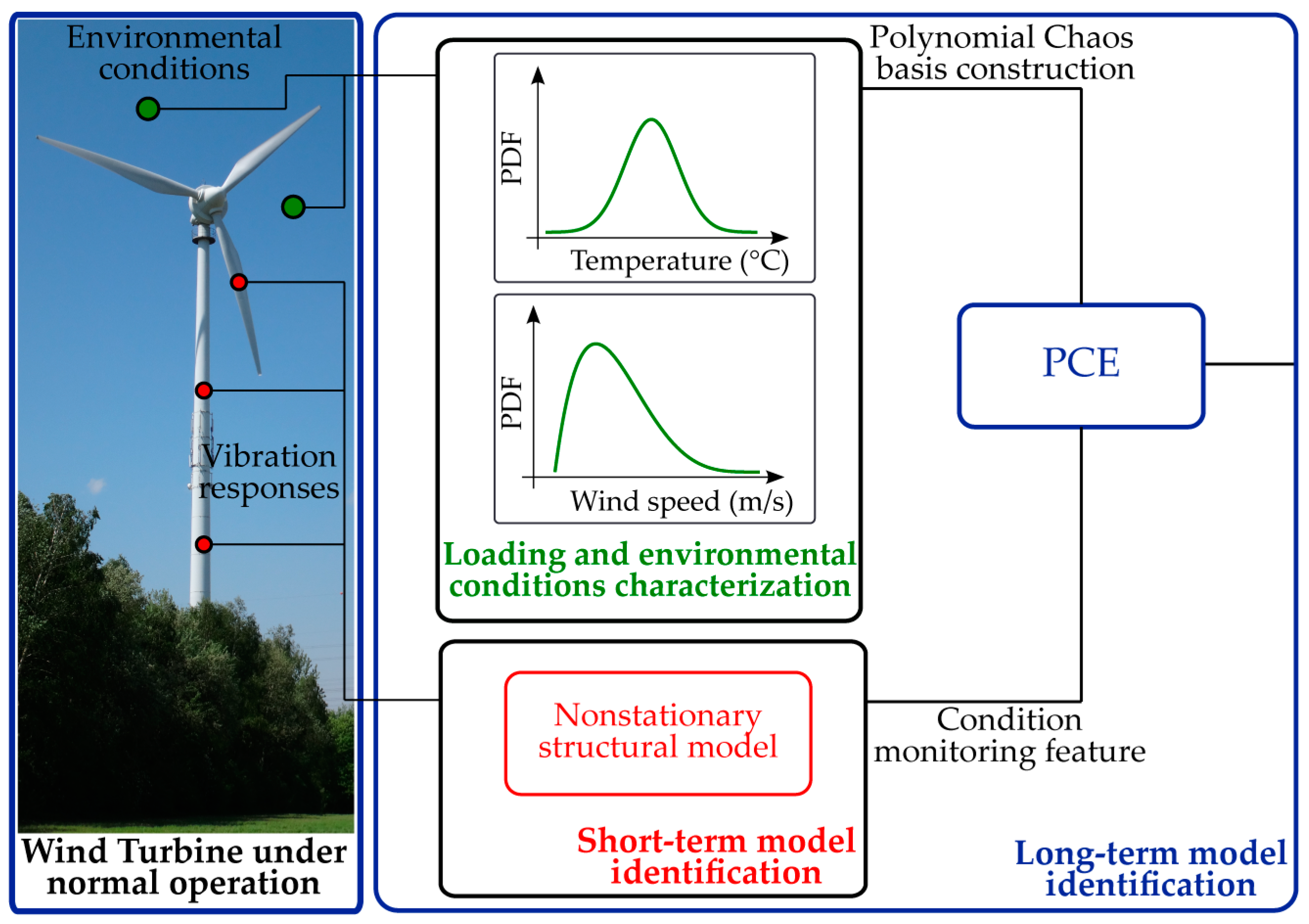
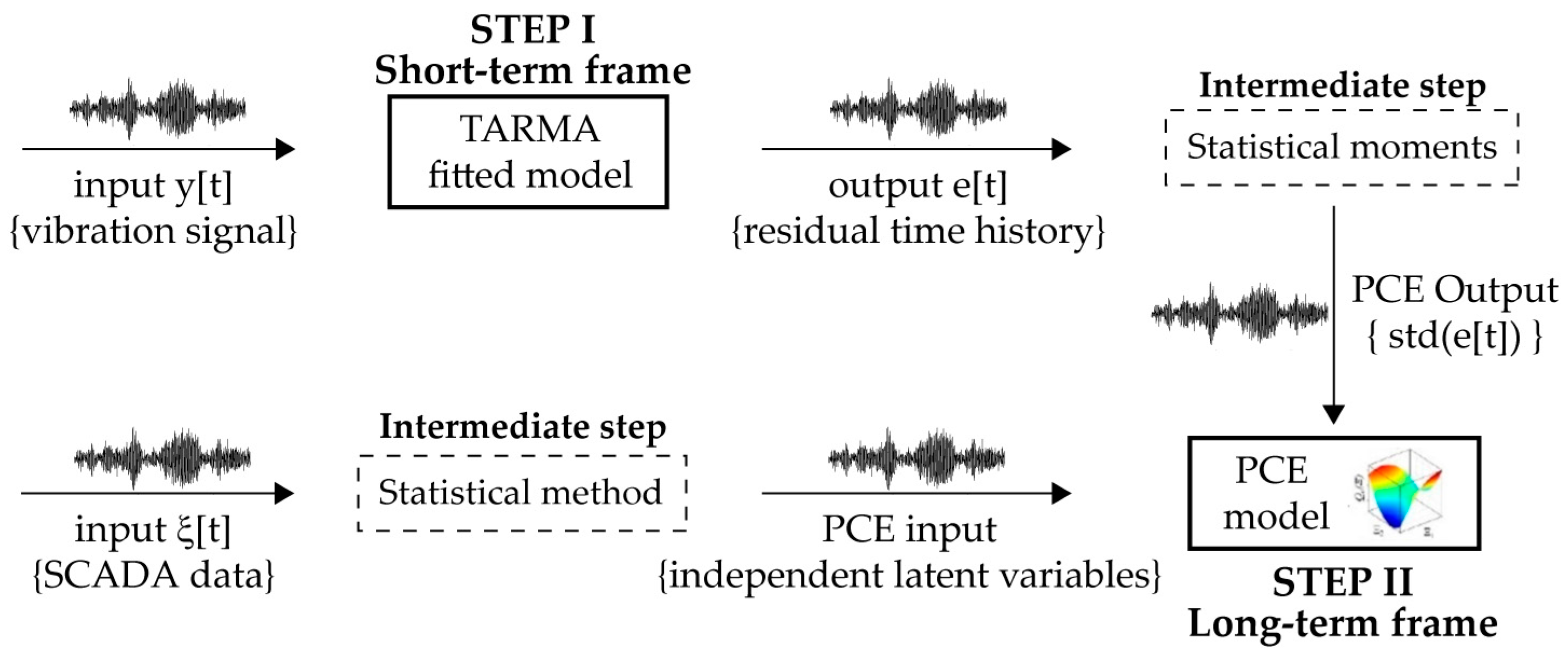
The long-term front is on the other hand focused on delivering the big picture, and therefore aims at accurate description of the WT dynamics over the complete operating spectrum of the structure. The typical stimuli linked to the long-term structural variability are changing within the range of hours, or even minutes and are usually related to changes in the wind flow profile, stochastic loads caused by wind turbulence, as well as variation of environmental conditions. For the purpose of modeling the evolution of the system response as a function of varying acting loads and operational conditions, the TARMA model is combined with the PCE method. The PCE model builds an expansion of a random output variable, e.g., an extracted TARMA model feature, on polynomial basis functions, which are orthogonal with respect to the probability density of the system’s random inputs, e.g., monitored environmental/loading parameters. The synergy between the two models enables a holistic assessment of a structure interacting with its environment. A schematic overview of the proposed strategy is presented in
Figure 1.
Considering for example a WT structure in regular operation, under the influence of ambient loading and changing environmental factors, a selected output feature (statistical moments of model residual) from the TARMA fitted model (step I) could be expanded on an appropriately constructed PC basis. By proper utilization of the TARMA model residuals (output parameter) and of the experimentally estimated operational and environmental variables (input parameter), the PCE model is finally constructed (step II). This coupled strategy provides the means for quantifying the uncertainty of WT dynamics due to randomness of the operational and environmental influencing factors. Furthermore, it delivers performance indicators in a standardized manner, which in turn contribute to development of a sophisticated damage detection strategy, where false fault alarms are timely recognized. An overview of the involved steps is presented in
Figure 2. The following sections summarize the theoretical background underlying these steps. For more detailed information on the applied models, the interested reader is referred to [
30,
31,
32,
33,
34,
35,
36,
37,
38,
39,
40].
2.1. Step I: Short-Term Framework
2.1.1. The Model Structure
For a non-stationary signal
the TARMA model, provides a compact parameterized formulation given in Equation (1), [
30]. Similar to the descriptive nature of its stationary counterpart (i.e., the ARMA model), the TARMA model describes a regressive form of the present output
on its past realizations
, taking into account modeling error and time-variability of the AR/MA parameters of the model:
where t designates discrete time (with
) of the observed nonstationary signal
,
is the residual sequence, i.e., the unmodeled part of the signal, assumed to be normally identically distributed with zero mean and time-varying variance
, and
,
the time-varying AR and MA parameters respectively, of AR, MA orders
.
In general, the identification of a specific TARMA model comprises two steps: (i) proper selection of the model structure (the
order for AR and MA parameters); (ii) estimation of the AR/MA parameters and the innovations variance
. However, for the specific subclass of smoothness-priors time-varying autoregressive moving average (SP-TARMA) models, the structure selection problem is further expanded to the selection of the smoothness constraints’ order
. The order
is directly related to an additionally imposed stochastic structure upon the AR and MA parameters. In order to constrain their time evolution, the SP-TARMA model enhances Equation (1) with the following set of supplementary stochastic difference equations, [
30]:
where
is the backshift operator
,
designates the difference equation order, and
is a zero-mean, Gaussian sequences with time-dependent variance, uncorrelated, mutually uncorrelated and also uncrosscorrelated with
.
Thus, the full SP-TARMA model may be completely described by: (i) a model for the system response y[t], Equation (1), and (ii) a model which controls the time evolution of the AR and MA parameters of the first model, Equations (2) and (3). The selected AR parameter order
represents the memory of the model and defines the number of past values of the signal, which are to be included into Equation (1). On the other hand, the stochastic smoothness constraints reflect our prior knowledge regarding the evolution of the underlying dynamics. The chosen order of the stochastic difference equations
introduces the number of past values of AR/MA parameters to be incorporated in the stochastic model of the constraints, and thus determines the behavior of the time varying AR/MA coefficients. For example for order
, the stochastic difference equations represent the random walk model, while for
each approximated AR/MA parameter locally follows a straight line and is distributed as a Gaussian white noise sequence [
31]. The time evolution smoothness of the AR/MA parameters is furthermore influenced, in a reciprocal sense, by the variance
. Therefore, a third user selected parameter, the residual variance ratio
, controls the equivalent memory of the estimation algorithm between the two limit values:
, which implies a locally deterministic (polynomial) parameter evolution, and
which implies no structure on parameter evolution [
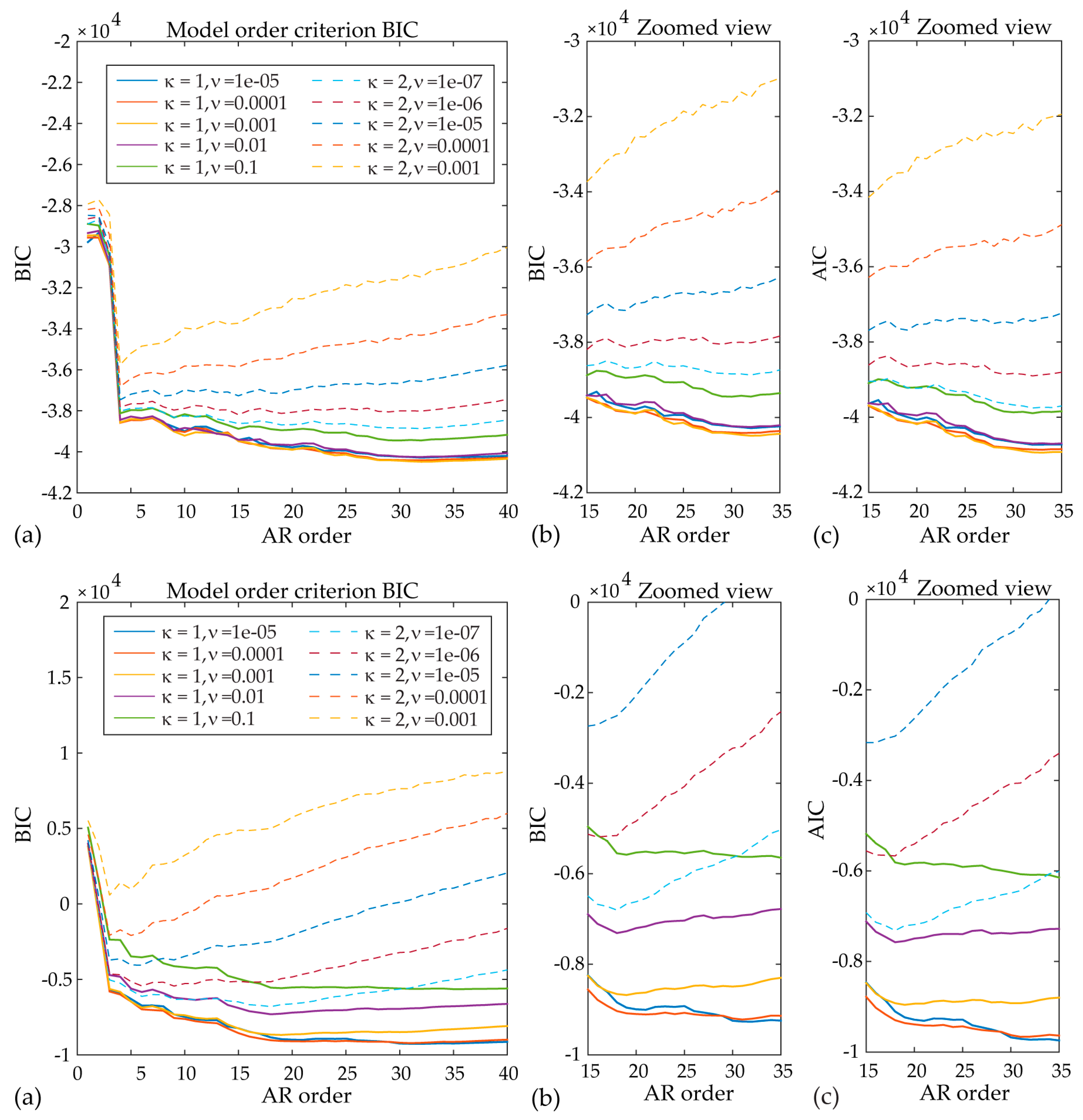
30]. An optimal value for
may be achieved by means of statistical approaches, such as minimization of the AIC (Akaike information criterion) or the BIC (Bayesian information criterion). Both criteria employ a penalty term that controls the increase of the model order, thus ensuring adequate modeling precision without overfitting the N-sample-long modeled signal
, Equations (4) and (5):
where
is the model likelihood,
N the number of signal samples, and
d is the number of independently estimated model parameters [
30].
2.1.2. Model Parameter Estimation
We reformulate the general (
-th order) smoothness constraints equations, Equations (2) and (3), in the following form:
where:
and
are matrices of the following forms (depending upon the value of
):
and so on,
designate the dimensional identity and zero matrices, respectively.)
The TARMA (
) representation of Equation (1) may then be expressed as:
with:
designates a vector containing all state vectors
up to time
.
Hence, the SP-TARMA (
) model may be completely expressed in state-space form, Equations (6) and (10). However, due to the unknown residual sequence
in
the full SP-TARMA case leads to a nonlinear state estimation problem. For this reason, i.e., for the recursive estimation of the state vector
, an Extended Least Squares (ELS)-like algorithm is employed. This leads to replacement of the theoretical prediction errors
in Equation (11) by their posterior estimates
, [
30]:
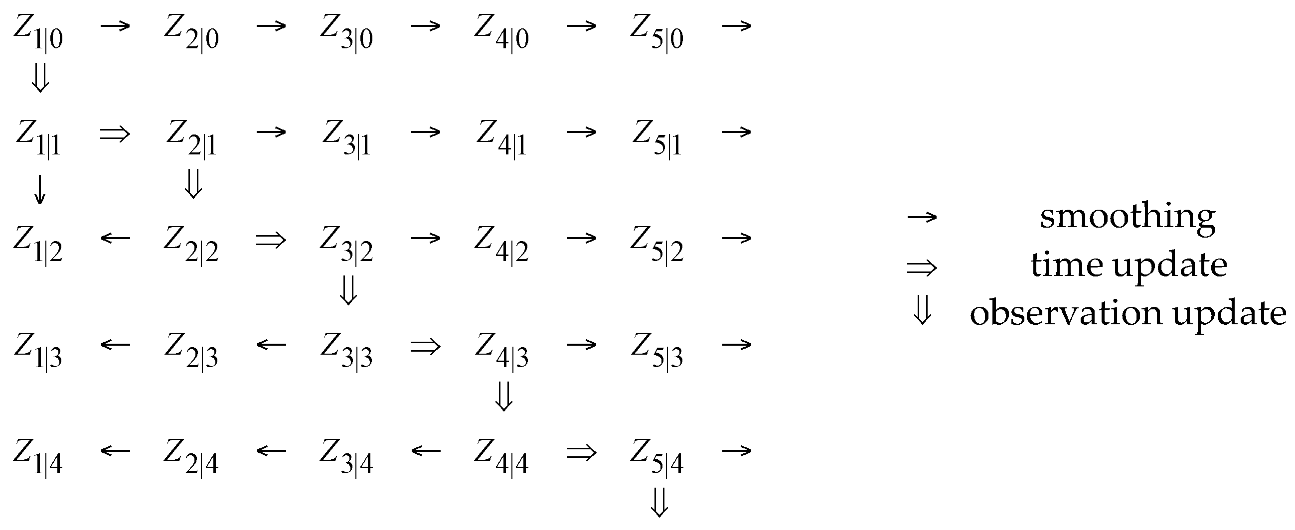
Then, for a given and time-invariant order κ and residual variance ratio
, the estimation of the state-space model may be achieved via the ordinary Kalman Filter (KF) scheme (
Figure 3). The innovations (one-step-ahead prediction error) variance,
, may be estimated via a window of certain length, centered at time instant
t, which slides over the prediction error (residual) sequence (more details and a summary of the normalized version of the KF method is provided in [
30]).
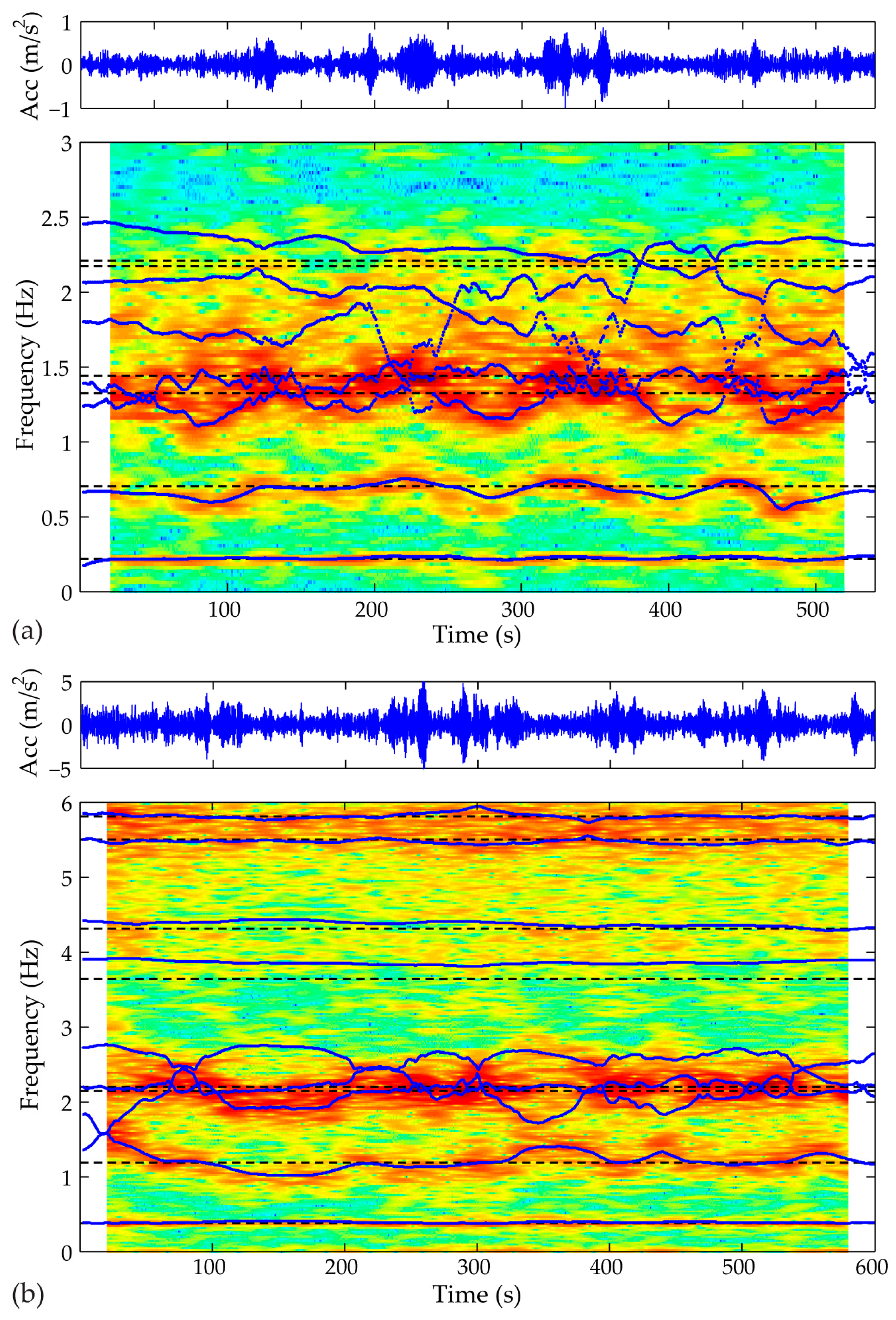
2.1.3. SP-TARMA Based Dynamic Analysis
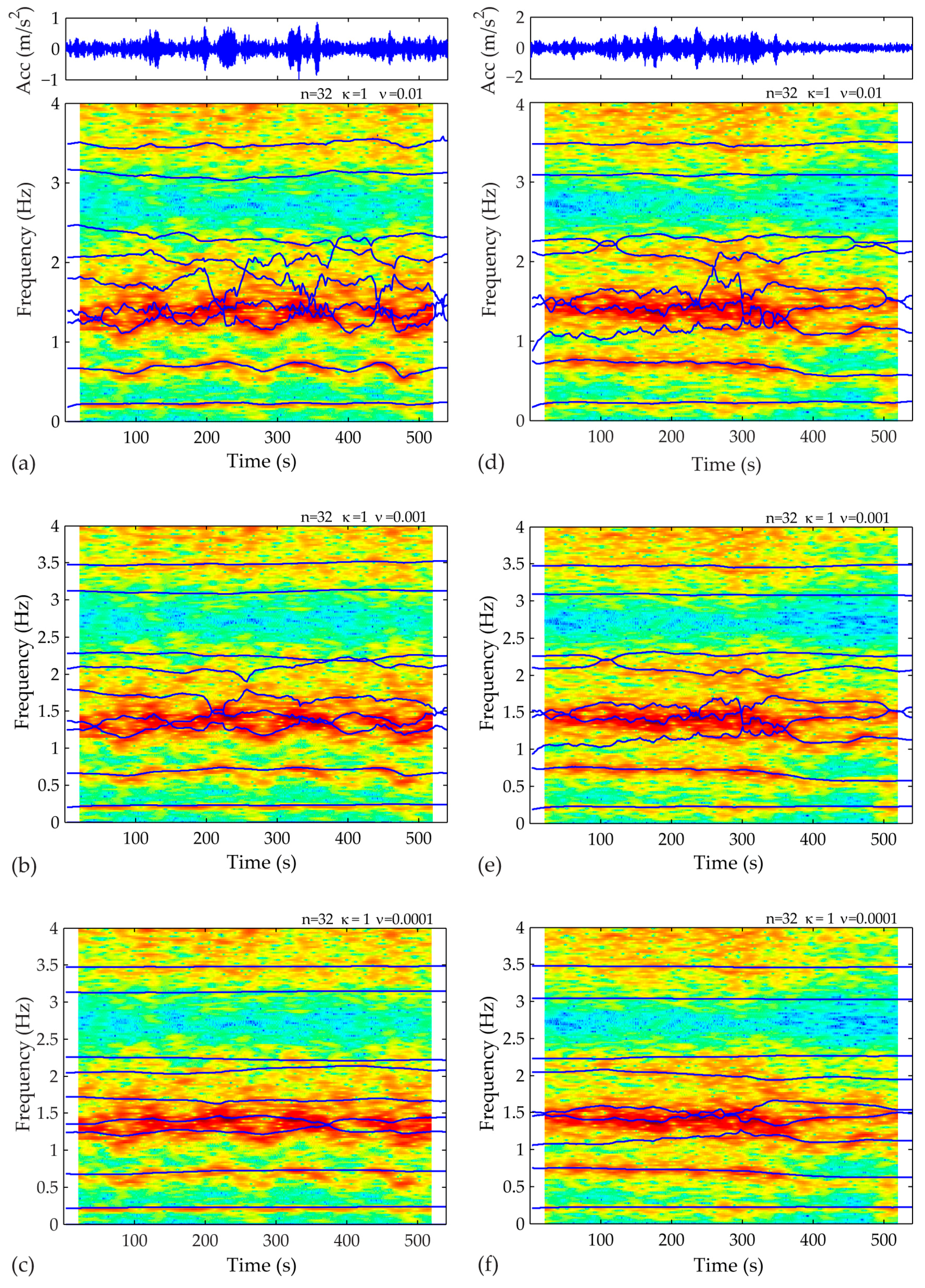
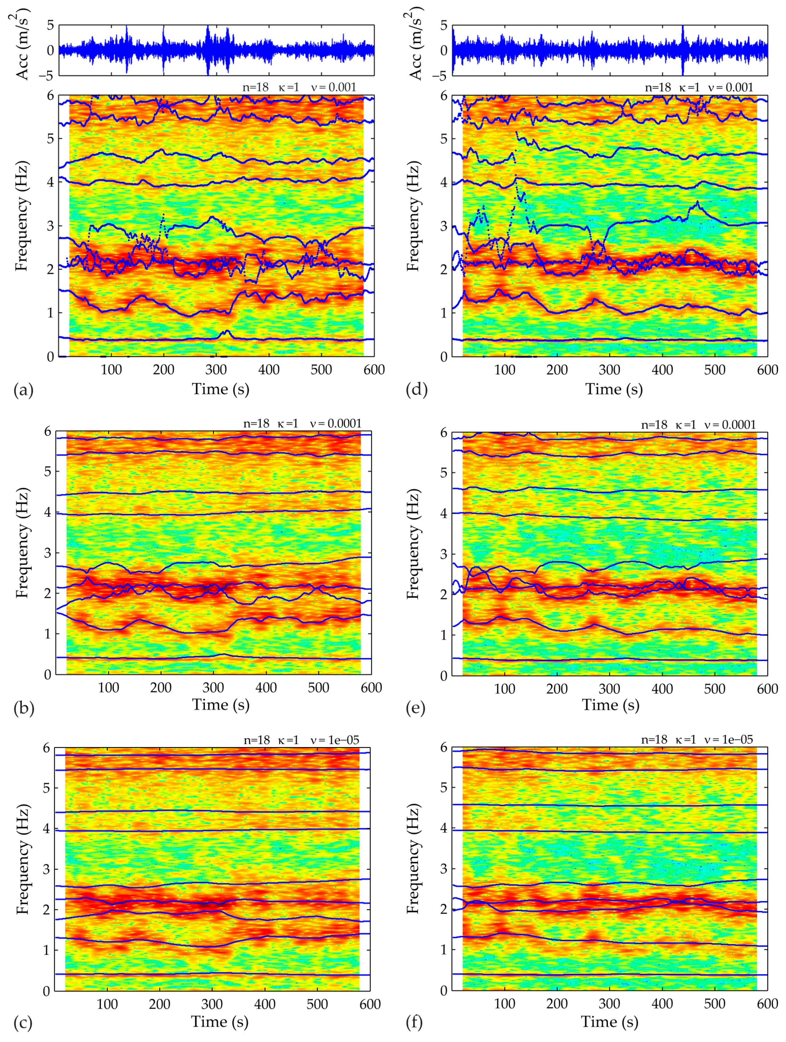
When the best-fit SP-TARMA model is identified, the time-varying dynamics of the structure may be recovered by the frozen-time spectrum [
30]:
where
is the frequency in rad/sec,
the sampling period in s, and
the imaginary unit. The frozen-time natural frequency
and damping ratio
of the system are related to the
discrete-time ‘frozen’ pole of the TARMA model’s frozen frequency response function:
2.2. Step II: Long-Term Framework (Modeling Uncertainty)
The time domain identification method described in
Section 2.1, accounting for the non-stationarity of the WT system, is combined with a PCE tool in order to deliver a SHM framework capable of describing the comprehensive structural dynamics, in a long-term scale.
In contrast to the local representative nature and high computational cost of the well-known Monte Carlo collocation method and other similar sampling techniques, the PCE non-sampling approach is focused on constructing a functional dependence of the model output on the set of independent random variables (RVs) (following a certain probability law) that parametrizes the input data, usually expressed in terms of a series [
33]. The polynomial chaos (PC) approach draws its origins in the modeling of stochastic processes via Gaussian RVs by employment of Hermite polynomials [
34]. Later on, Cameron and Martin [
35] demonstrated that for any arbitrary stochastic process with finite variance, the PC expansion converges in the
sense. The latter was generalized by Xiu et al. [
36] to different continuous and discrete distributions using orthogonal polynomials of the so called Askey-scheme [
37].
The main concept underlying the PCE framework is to represent a random quantity by means of expansion, comprising functions of random variables multiplied with deterministic coefficients. More precisely, PCE modeling generates an expansion of a random output variable on polynomial chaos basis functions, which are orthonormal with respect to the probability space of the system’s random inputs. For a system S featuring M random input parameters represented by independent random variables
, gathered in a random vector
of prescribed joint Probability Density Function (PDF)
, the system output, denoted by
, will also be random [
38]. Provided that Y has finite variance, it can be expressed as follows:
where
are unknown deterministic coefficients of projection,
is the vector of multi-indices of the multivariate polynomial basis (PC functions)
, orthonormal to
. The PC polynomials are chosen so that the weights
which ensure the orthogonal property.
, resemble the PDF of the random variables. Several well-known families of orthogonal polynomials can be associated to a specific PDF, a more detailed overview may be found in [
36].
The multivariate polynomials
used for constructing the PC model (for each term j of the PC series expansion) are obtained by tensor products of the corresponding univariate functions:
where
M is the number of random input variables.
For ensuring timely computation, the functional series terms Equation (16) must be truncated to a finite number. The usual approach is the selection of the multivariate polynomial basis with total maximum degree
. In this case the dimensionality of the functional subspace, i.e., the total number of series terms, equals:
where P is the maximum total degree of the multivariate polynomials. The truncated PCE model of Equation (16) to the first T terms yields a finite number of deterministic coefficients and the parameter vector
may be estimated by solving Equation (16) in a least squares sense [
38].
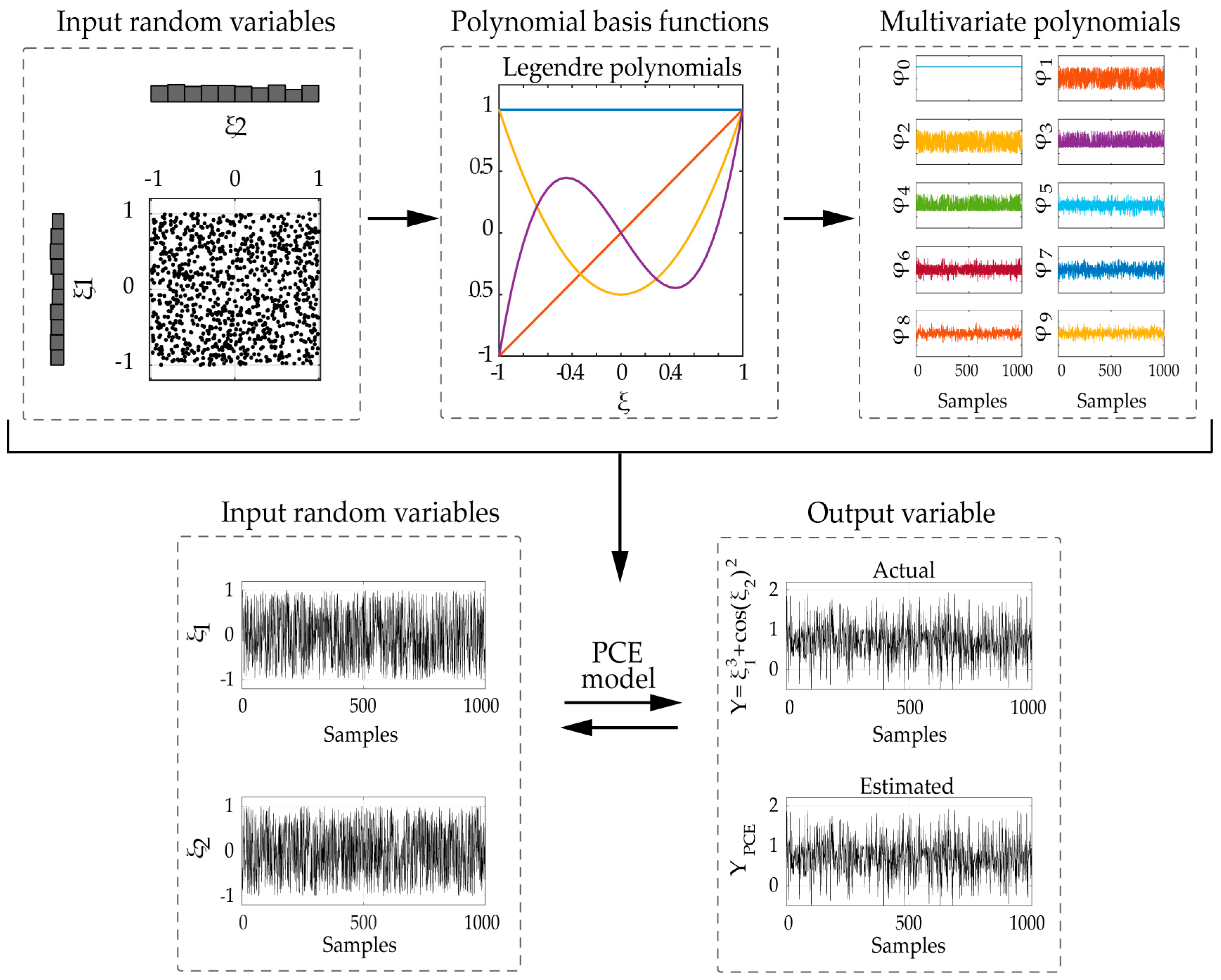
For illustrating the construction of the PCE model, let us consider the simple case of a 2D-PCE model for two independent input random variables
. By employing the first four univariate Legendre polynomials as PC basis functions for a selected total degree P = 3, we may develop the truncated PC expansion of Equation (19) (total number of terms T = 10, single index notation used). The construction of the 2D polynomials is presented in more detail in
Table 1, and a schematic overview of the complete method is presented in
Figure 4.
It is worth mentioning that in case of subpar performance of the standard PCE due to the rather limiting assumption of prescribed families of input distributions, an arbitrary or adaptive PCE scheme could serve as viable alternatives [
33,
38,
39]. Unlike the classical approach, which utilizes a fixed form of PC basis functions, these variants employ PC functions adapted to the specific input variable characteristics.
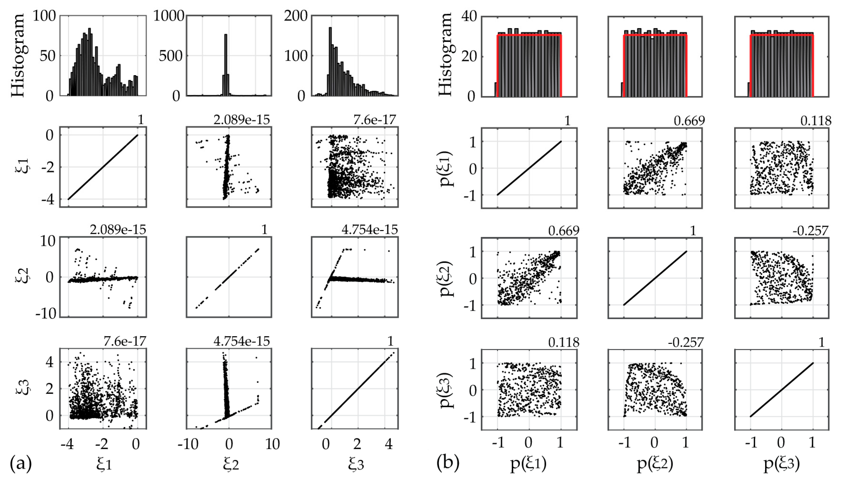
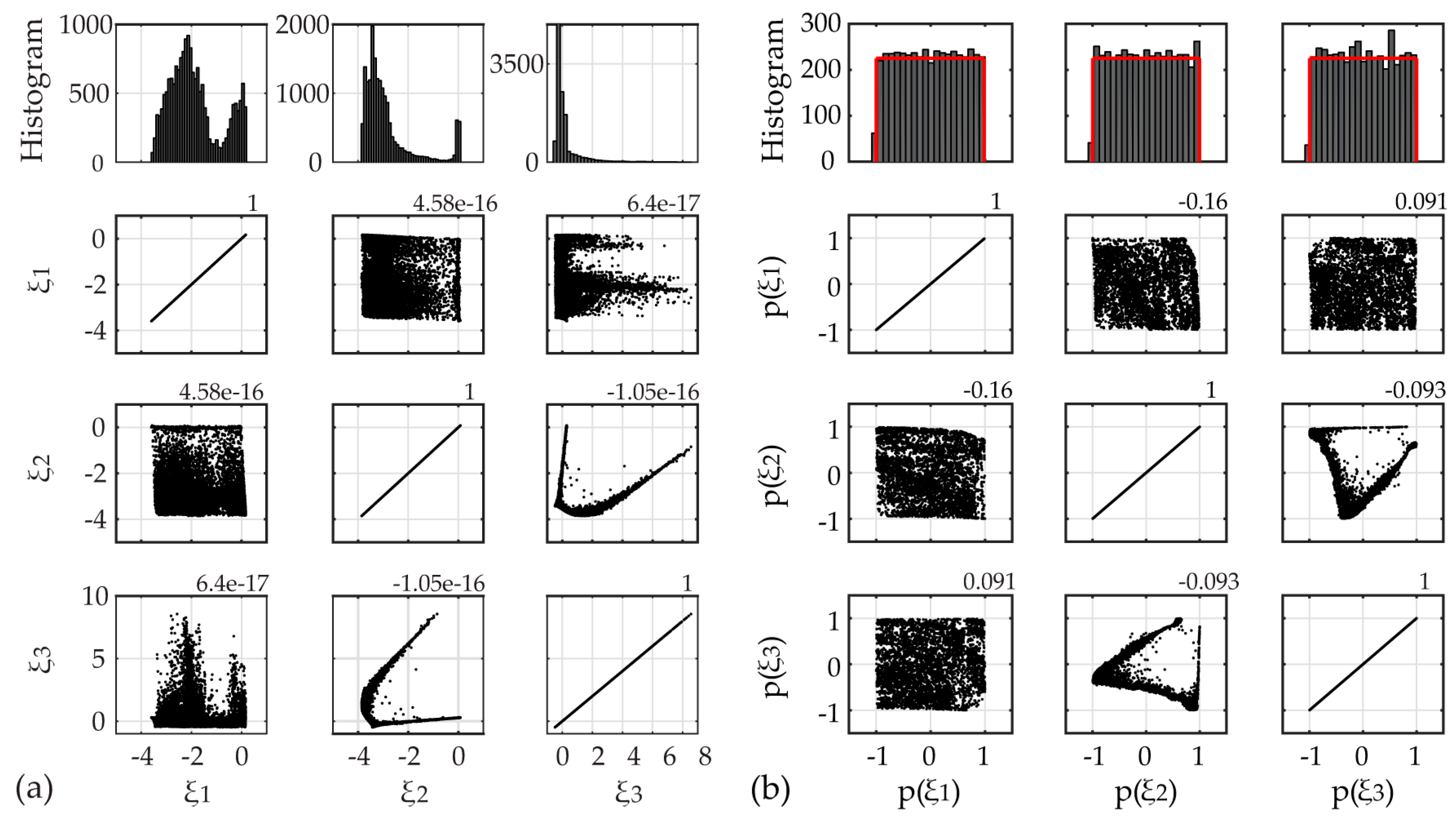
Probabilistic Approximation of Random Variables
The prerequisite of independent input parameters, necessary for efficient PCE modeling, is here ensured by utilization of a statistical technique capable of inferring independent (latent) variables that are intermixed within observed data. Independent Component Analysis (ICA) is a computational approach that in contrast to Principal Component Analysis is concerned with the higher order statistics of the observable data, i.e., minimization of mutual information. ICA eventually aims at identifying non-Gaussian and mutually independent components [
40], which may then be fed into the PCE component of the proposed SHM framework.
The basic concept of ICA is in fact to describe how an observed random vector
is generated by a process of mixing unobservable (latent) variables. More specifically, if we consider
observed linear mixtures of n independent components
(
) the following relation is assumed [
40]:
or by using vector-matrix notation:
with
designating the random observed variables vector,
the vector of unobserved independent variables and
A the unknown mixing matrix:
Via inversion of the mixing matrix
, the vector of the independent latent variables
becomes:
ICA employs nonlinear optimization for estimating the mixing matrix
A, which maximizes the non-Gaussianity of each one of the latent variables
(with
designating a column vector of matrix
). The adopted measure of non-Gaussianity, may be based on kurtosis, negentropy, and others [
40]. A concise overview of the method, as well as a comprehensive flowchart of the ICA algorithm is presented in [
23].
4. PCE-TARMA Diagnostic Index
The SHM-based system diagnostics is built on training data from the baseline, or “healthy” structure under regular environmental and operational conditions. The obtained models are then implemented with newly acquired data, and deviations from the established normal conditions are detected as a novelty [
28]. A robust diagnostic tool should be able to distinguish between true system changes and benign alarms, originating from new ranges of measured input data. In this case, instead of alarming for a potential maintenance intervention, model retraining should be carried out on the basis of the extended data set.
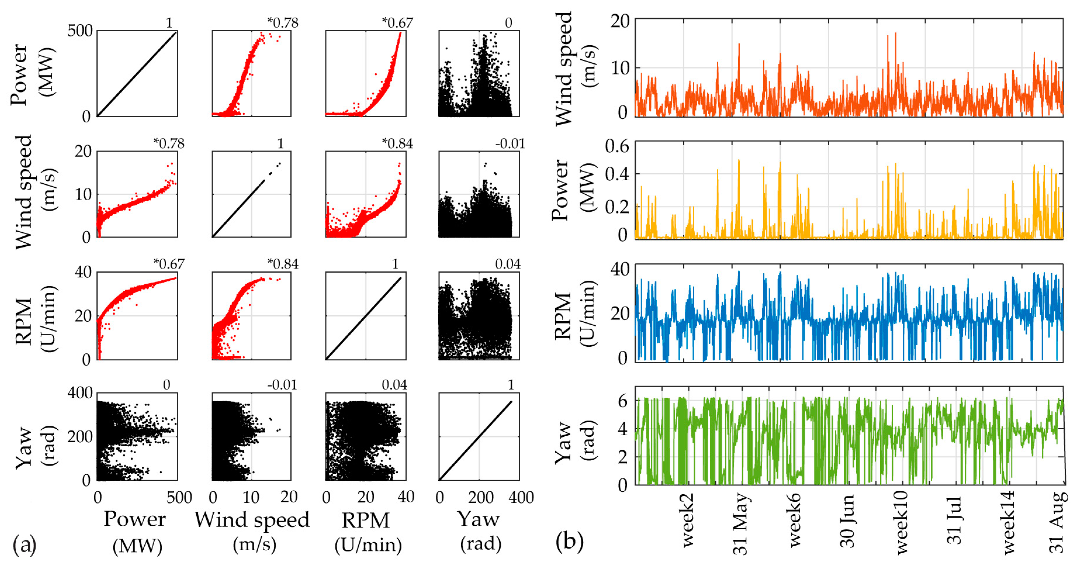
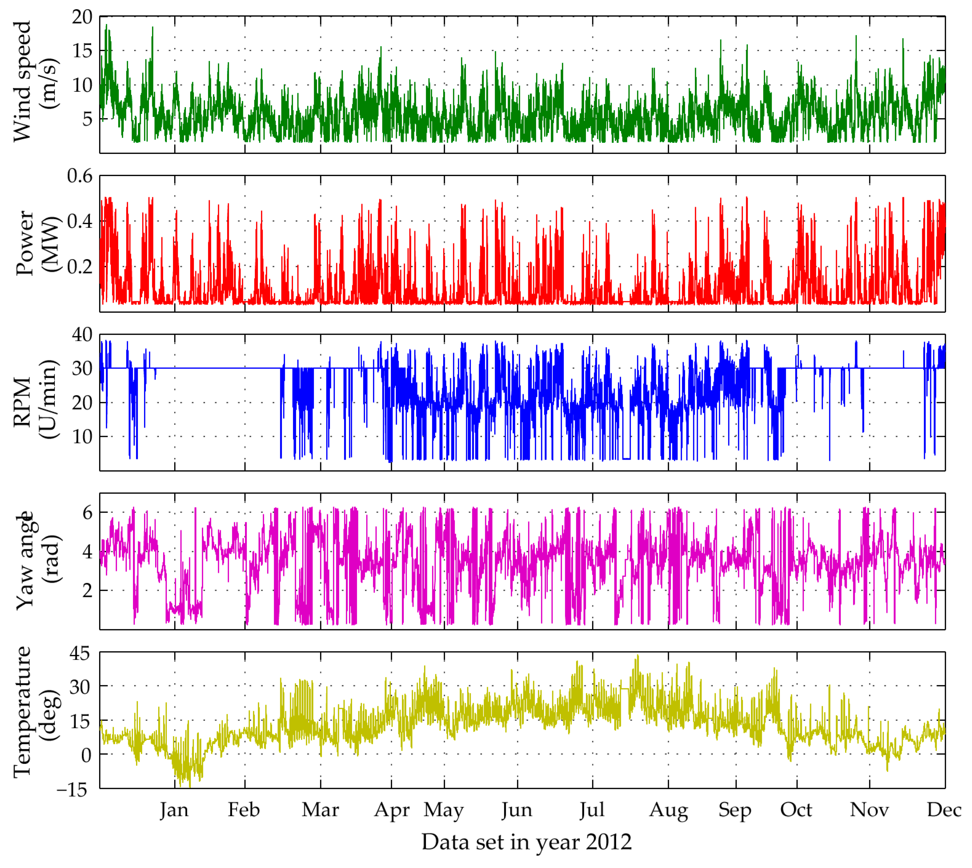
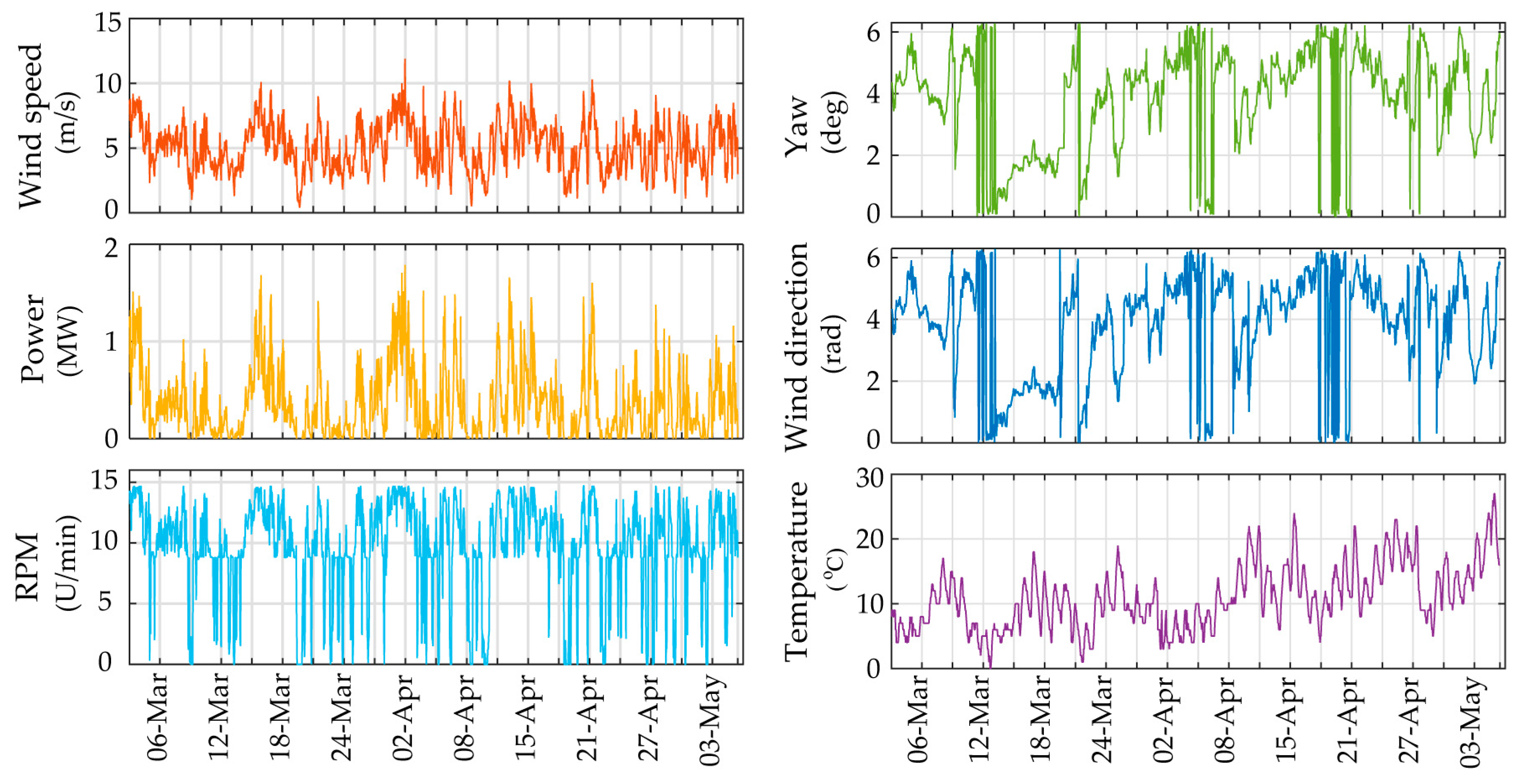
In this context, the developed PCE-TARMA model responsiveness to varying environmental and operational parameters (EOP) is tested for two, three and four-month long training periods, with an input of five distinct SCADA variables (
Figure 18). Based on the previously described framework in
Section 3, the long-term tracking is extended to one complete year time-frame of monitored data for the operating Case B WT structure. The PCE-TARMA model is refitted with the model parameters summarized in
Table 2,
Section 3.4. During the twelve-month tracking period influencing agents characterized by seasonal variations would bear a significant impact. Therefore, in this setting the temperature measured at the outer side of the WT tower shaft (at 20 m height) is incorporated as a PCE model input as well.
In
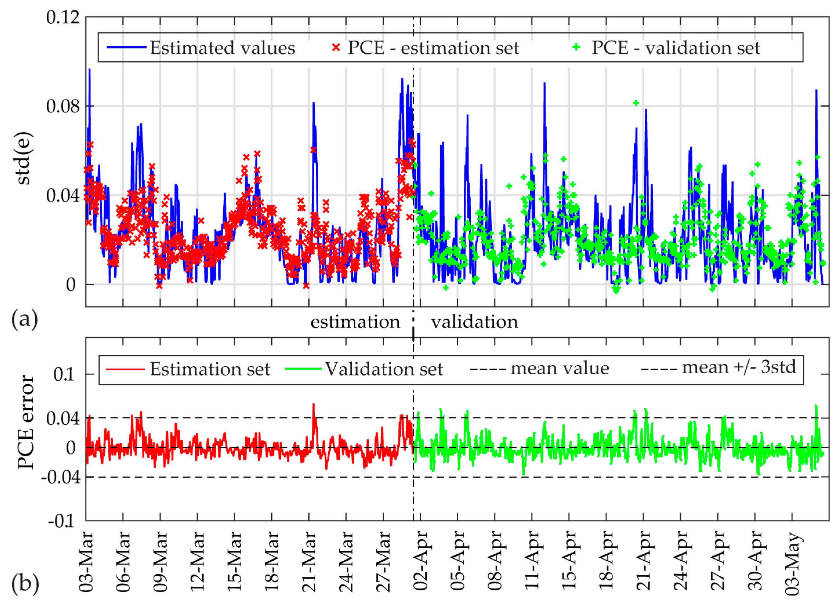
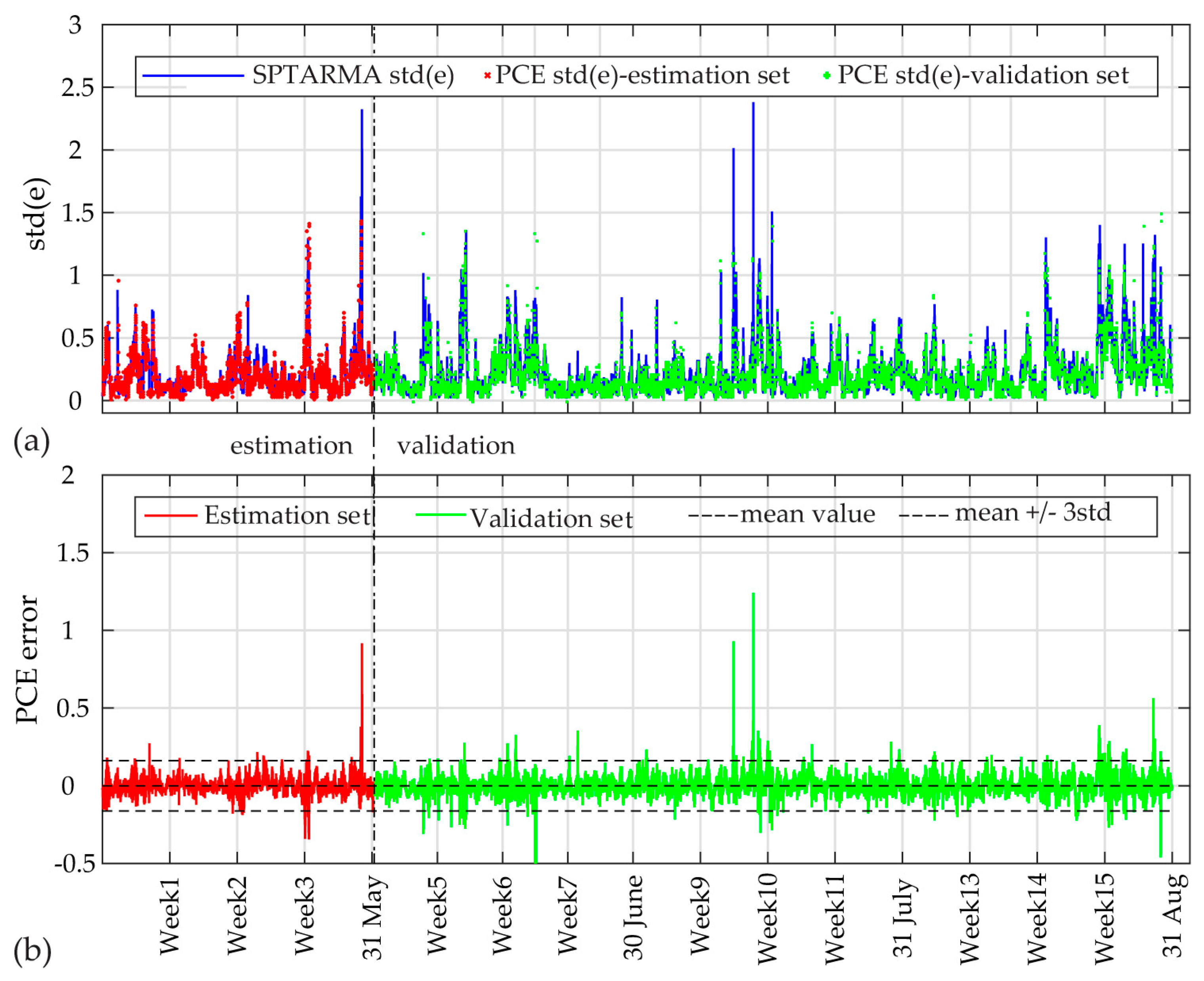
Figure 19,
Figure 20 and
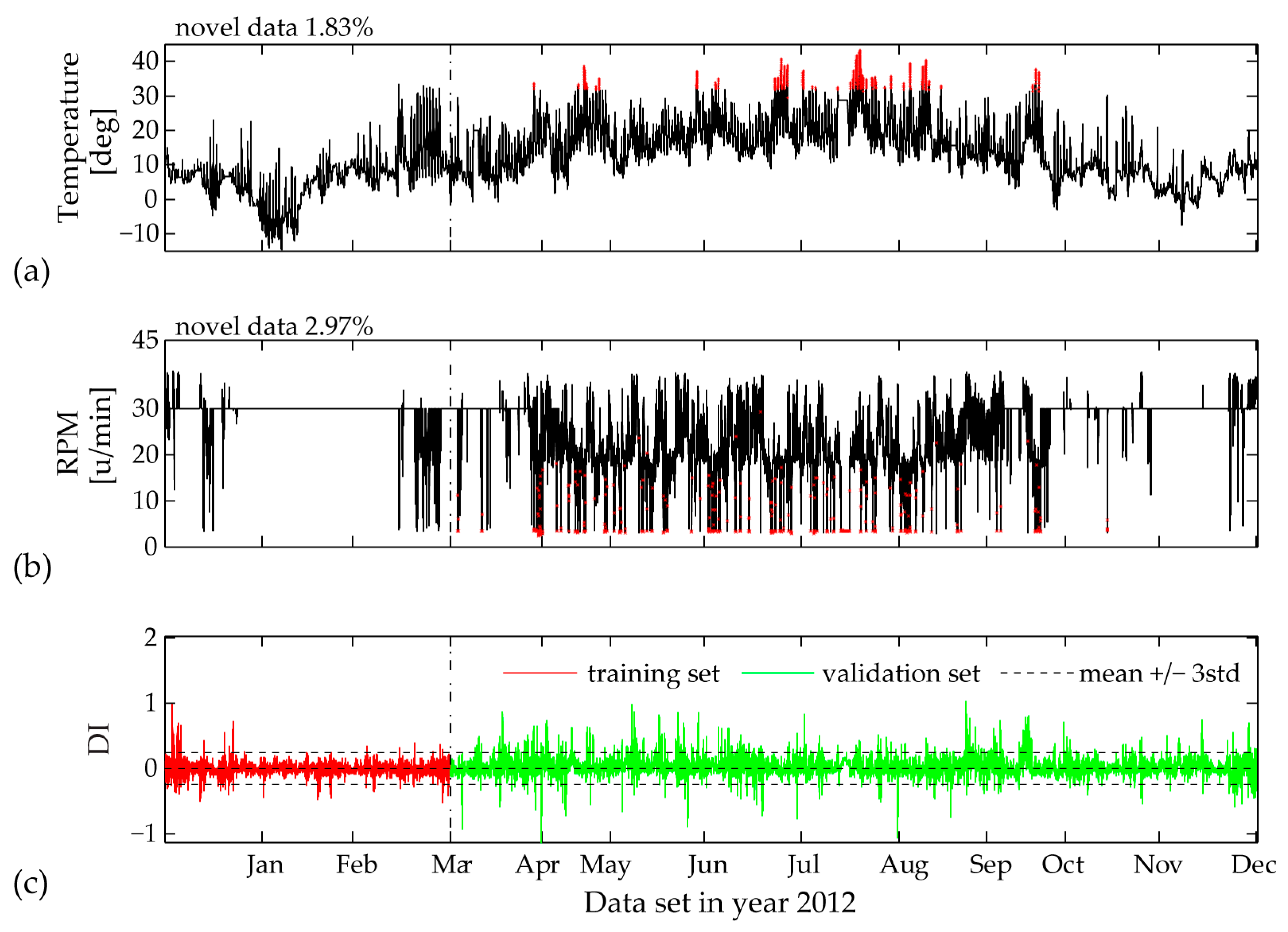
Figure 21 the validation sets of the estimated PCE residual demonstrate the workings of a consistent Diagnostic Index (DI) able to directly illustrate unfamiliar fluctuations in the EOP. Following statistical outlier analysis the index values which exceed the thresholds of ± 3std can be linked to new data ranges of measured influencing agents.
For this purpose, the well-known Mahalanobis Distance (MD) method is herein applied on the input data time histories. For a p-dimensional multivariate sample
, the MD is defined as, [
42]:
where
is the arithmetic mean and
is the sample covariance matrix, both estimated for an input data set corresponding to a certain training period length. For normally distributed multivariate data, the MD values result approximately chi-square distributed with
degrees of freedom
, while the MD threshold is usually set as a certain quantile of
. However, an adaptive method that takes into account the actual empirical chi-square distribution function of the estimated MD (instead of a fixed quantile) is herein applied [
42]. In this way thresholds (adjusted quantiles) are estimated for corresponding training sets for each of the five SCADA parameters. The
samples from the validation sets which have MD beyond the predefined threshold are defined as novelties.
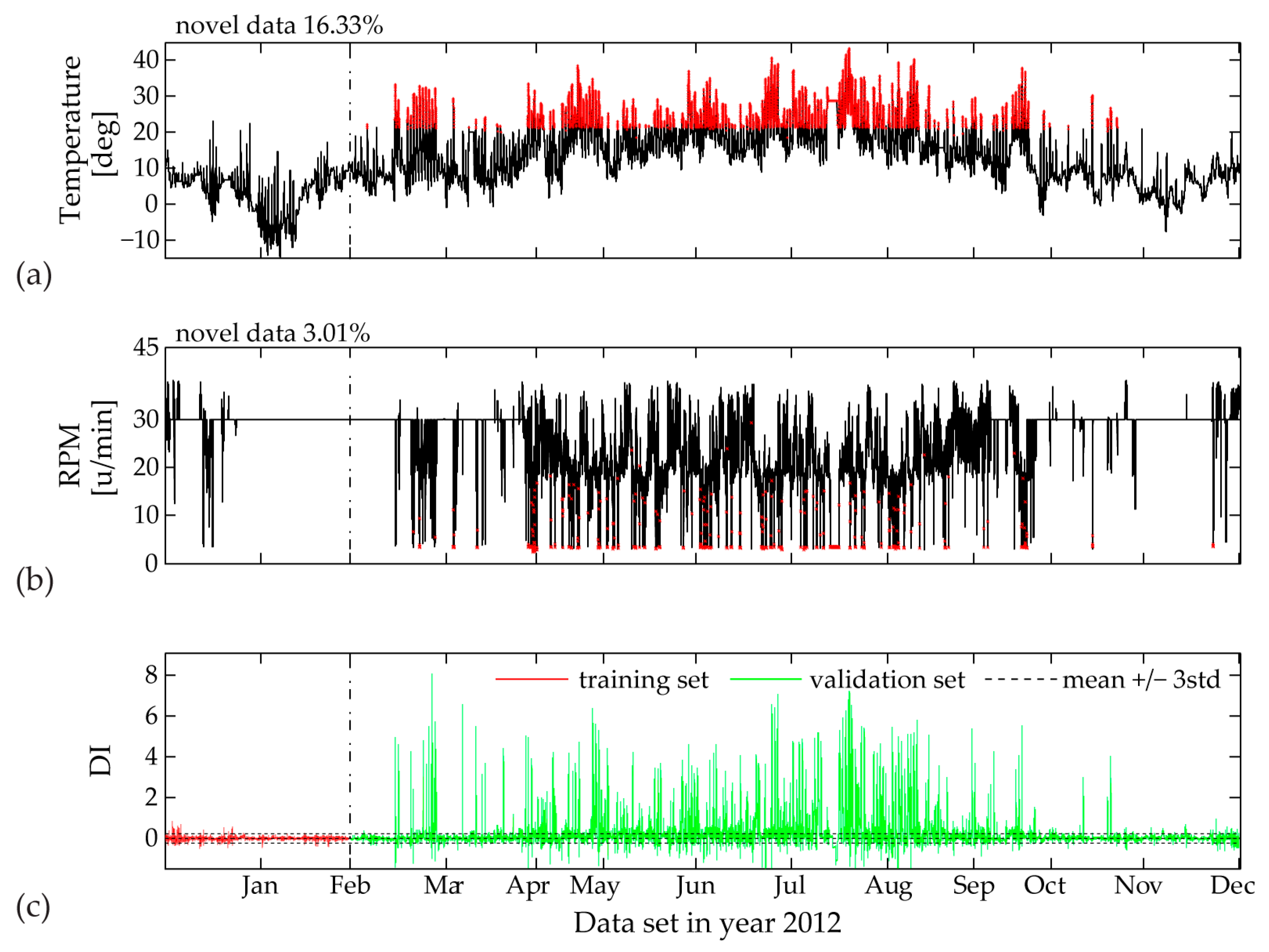
False triggering alarms due to incomplete training set are mostly related to input parameters characterized by unpredictable range of values, i.e., temperature measurements and wind velocity. In this case for a two-month training period, the univariate MD plot of the temperature time history shows the highest percentage of 16.33% novel data (
Figure 19). The DI distribution pattern, plotted in the same figure, is clearly linked to the new upcoming values between months March and November. If we further increase the training set to a three-month period (
Figure 20), the MD outlier percentage for measured temperature decreases. Correspondingly, the DI becomes significantly reduced, although not yet within the ± 3std limit values. In
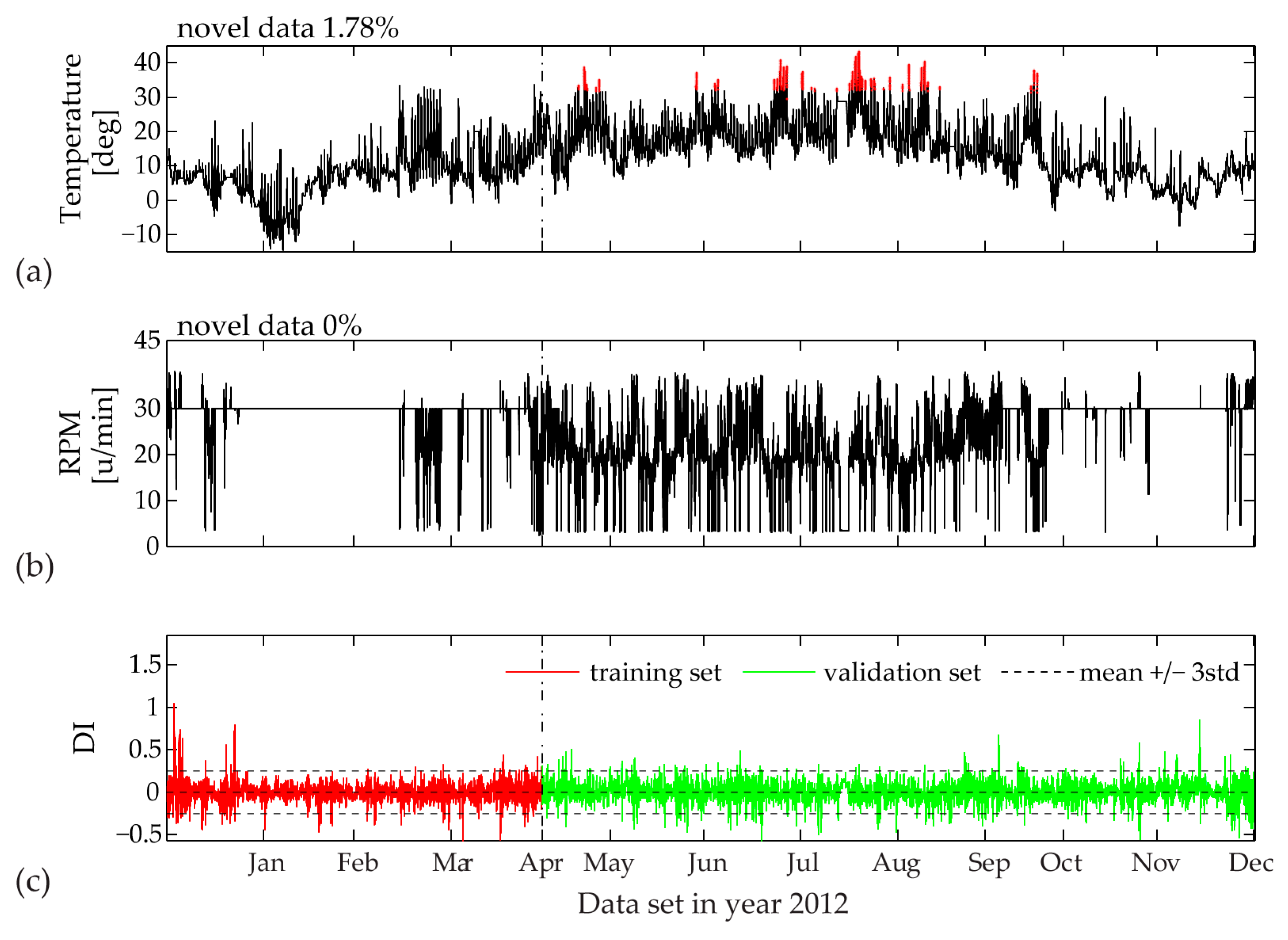
Figure 20, for the same three-month training period, an interesting observation is the contribution of the rotor rotation to novel data (2.97%), which is completely reduced to 0% after four months of model training (
Figure 21). The reason for this occurrence is the relatively flat range of RPM values between mid-January and mid-March, most probably due to a sensor malfunction, which later on is repaired.
The MD plots (
Figure 20 and
Figure 21) demonstrate that for a full incorporation of various fluctuations in the measured temperature, the training period should be even extended to eight months. Additional univariate MD analysis for the measured wind velocity, power production and yaw angle for the complete year 2012 reveals no new data points within the validation sets of these inputs, even for a training period lengths of one to two months (January and February). The estimated minimum PCE model training set lengths for capturing the complete scope of the separate SCADA variables is summarized in
Table 3.
6. Conclusions
Europe’s growing needs for energy savings have placed WT structures in focus, albeit the tackling of complexities of these structures has long occupied both the academic and industrial communities. At the same time, the recent technological developments in sensors and monitoring solutions motivate the enhancement of the currently adopted SCADA stream for WTs with information of structural nature, able to guide operators in the management of these assets.
In materializing such a goal, it is important to account for the non-stationary response of operating WTs and the temporal variability of their identified modal parameters. In order to develop comprehensive dynamic models both issues need to be addressed. By merging environmental and operational variables with a time-varying model of vibrational response, the proposed bi-component tool serves as the first step towards automated condition assessment.
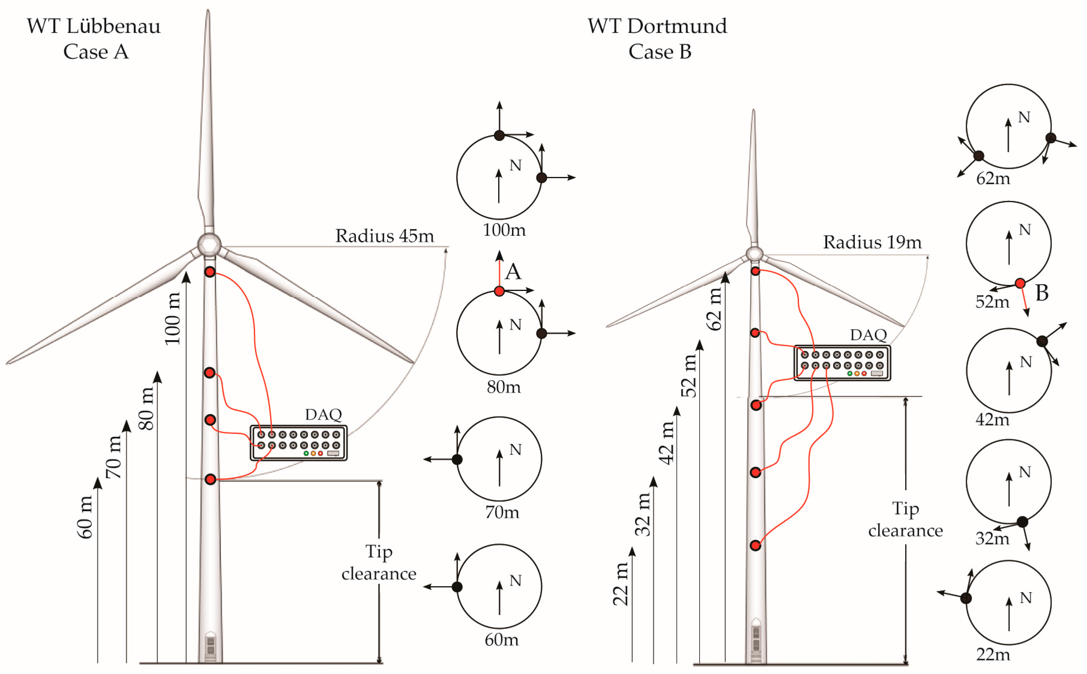
Successful implementation of the devised strategy on two distinct operating WT structures in Germany for different settings, namely, different sites, turbine types, SCADA duration, and different influencing agents, verifies the robustness of the approach. Furthermore, the outcomes of the complete one-year tracking of the obtained diagnostic index demonstrate the potential of the proposed tool for incorporation within a holistic SHM damage detection framework, further extended via statistical pattern recognition methods, to be explored in a next step. Another interesting perspective lies in fusing the surrogate models developed as part of this diagnostic framework with a simulation-based design procedure, where simulations of the SP-TARMA model for diverse loadings may be used for predictions on processes such as fatigue, equivalent damage loads, etc.


 ,
, 


